An ANN Hardness Prediction Tool Based on a Finite Element Implementation of a Thermal–Metallurgical Model for Mild Steel Produced by WAAM

Abstract

WAAM has emerged as a promising technique for manufacturing medium- and large-scale metal parts due to its high material deposition efficiency and automation level. However, its high heat accumulation and complex thermal evolution strongly affect the resulting microstructures and mechanical properties. The heterogeneous and unpredictable nature of these properties hinder the widespread application of WAAM in the steel construction industry. In this study, an artificial neural network (ANN) hardness model is developed, based on a thermal–metallurgical model for mild steel. The objective is to establish non-linear relationships between the input process parameters and the desired output, i.e., hardness. The thermal–metallurgical model utilizes a well-distributed heat source model, a death-and-birth algorithm, and a metallurgical model to simulate the temperature field and to calculate the microstructure phase fraction. The temperature prediction errors at four thermocouple positions are mostly below 20%. Because of the limited experimental data, twenty-five simulation experiments are performed using the L25 orthogonal array based on the Taguchi method. The analysis of variance (ANOVA) reveals that the travel speed has the greatest impact on hardness. With the dataset from the thermal–metallurgical model, an ANN model to predict hardness is developed. A comparison to experimental data shows excellent performance and accuracy, with the Mean Absolute Percentage Error (MAPE) of ANN predictions within 10% of the targeted hardness.

1. Introduction

There is a growing interest in advanced additive manufacturing methods, in both research and industry. Within the realm of metal component manufacturing technologies, Directed Energy Deposition (DED) has emerged as a prominent technique, wherein focused thermal energy is utilized to fuse materials by melting them during deposition. DED encompasses various methods, including both wire-feed and powder-feed processes. One notable variant is Wire Arc-Directed Energy Deposition (WA-DED), also named Wire Arc Additive Manufacturing (WAAM), which employs an electric arc as the heat source and utilizes a filler wire to deposit layers of metals. WAAM has attracted significant attention for its capability to produce medium- to large-scale components. This is because of the advantages such as an elevated deposition rate, flexible building volume, high material deposition efficiency, and the low cost of equipment investment, as well as raw material [1,2,3]. However, the high heat accumulation and the complex thermal evolution during the deposition strongly affects the microstructures and the mechanical properties of the as-built component [4,5,6], as well as the residual stresses [7]. These effects are generally investigated using experimental methods. A large number of experiments would be required to establish the relationship between the process parameters (including welding current, voltage, travel speed, and the chemical composition of the filler wire) and the resulting microstructure, as well as mechanical properties. However, due to the high costs involved (especially for large-scale components), only a limited number of well-documented experimental datasets have been reported in scientific literature [8,9,10]. These limited experimental results are insufficient to reveal the complex process–structure–property relations in the WAAM process.

To overcome the above-mentioned challenges, recently, thermal–metallurgical models, based on finite element simulations and the empirical phase transformation theory, have been developed to simulate the temperature distribution, phase fraction evolution, and hardness distribution in the WAAM deposits. For instance, Mehran et al. [11] developed a thermal–metallurgical-mechanical finite element model to accurately simulate the single bead-on-plate welding of an ultra-high strength carbon steel. This model includes comprehensive solid-state phase transformation modeling, covering both diffusive and displacive transformation kinetics. For diffusive transformation, the kinetics model of Machnienko was utilized, while the Koistinen–Marburger kinetics model was employed for martensitic transformation. The Koistinen–Marburger model was based on an experimentally determined Continuous Cooling Transformation (CCT) diagram. However, the experimental cost associated with determining the CCT diagram limited the applicability of the simulation tool. To overcome this problem, Mi et al. [12] implemented a different calculation model to consider the phase transformations of Q235 steel during a laser welding process. However, the complex calculation methods and the large number of empirical parameters inherent to this approach limit its widespread application. Consequently, despite its lower computational accuracy compared to the aforementioned models, Lusk et al. [13] adopted a traditional calculation method, which includes line interpolation and the Johnson–Mehl–Avrami–Kolmogorov (JMAK) equation, to faster calculate the phase transformations during WAAM.

It is evident that numerical simulation offers the capability to predict the outcomes for various configurations of process parameters at a lower cost compared to the experiments. However, its extensive computation time limits its further application. To address this challenge, predictive models based on machine learning have been developed, allowing us to rapidly predict the thermal history and the geometrical information of WAAM deposits for the given process parameters [14,15,16,17,18,19,20]. For instance, Van et al. [18] built a prediction model for the WAAM thermal history via a feedforward neural network-based surrogate model (FFNN-SM). The developed FFNN-SM model can accurately estimate the temperature evolutions at different sample positions, whilst saving 99.75% time compared to the finite element (FE) simulations. Pant et al. [19] adopted artificial neuron network and particle swarm optimization (PSO)-ANN algorithms to predict the clad characteristics of a laser metal deposition process, based on a small dataset. PSO-adaptive neuro-fuzzy inference system (ANFIS), as well as genetic algorithm (GA)-ANFIS prediction models were designed by Xia et al. [20] to predict the surface roughness of a WAAM component. The authors concluded that the prediction models have a high prediction performance and low computational cost.

The above review of the literature indicates that machine learning-based predictive models can help researchers in developing non-linear mathematical relationships between WAAM process parameters (e.g., voltage, current, travel speed, wire feed rate, cooling time) and desired outputs (e.g., mechanical and geometrical properties) with a lower cost and computation time compared to an experimental- or FE-based approach. However, to the best of the authors’ knowledge, there is not yet a prediction model revealing the relationship between the process parameters and the hardness of WAAM component. Additionally, there is no systematic research developing prediction models that combine generated data (through FEA and experiments), the design of experiments, and data processing through ANN. Inspired by the above-mentioned publications and their related theories, this study develops an ANN hardness tool for mild steel produced by WAAM. The developed model facilitates the rapid establishment of non-linear mathematical relationships between the process parameter inputs (travel speed, wire feed rate, and cooling time) and the desired output, i.e., hardness, with the lowest experiment cost and computation time. For this purpose, a thermal–metallurgical model is implemented in finite element software and a Taguchi design of experiments is used to generate a dataset for training the ANN model.

The global framework of the developed analysis procedure is shown in detail in Figure 1. The heat transfer analysis, the phase transformation-based metallurgical model, and the ANN prediction model are performed in the FE software ABAQUS 2019 and MATLAB Research R2018 platform, respectively. Using the well-distributed volumetric heat source and the element birth-and-death approach, both a single-pass and a multi-layer WAAM process are numerically analyzed. The accuracy of the thermal analysis model is validated by comparing the simulation results with the experimental data reported by Ding et al. [21] at four different thermocouple measurement positions. First, the nodal temperatures are extracted from the results datafile via Python scripting. Next, for the material points that underwent transformation, the relevant kinetics model (implemented in the MATLAB platform) is applied to obtain the volume fraction of austenite during the heating process and the transformed phases upon austenite decomposition during the cooling process. In this context, equations are implemented to determine the variation of hardness and the phase volume fractions at each node and time increment. After that, the results of phase volume fractions are employed as solution-dependent state variables (SDVs), and an input file for ABAQUS is rebuilt to simulate the influence of a change in phase fractions on the temperature variation, and to obtain updated results including temperature, phase fractions, and hardness. The developed thermal–metallurgical model is then employed as a tool to perform a series of numerical experiments designed by the Taguchi method. Finally, the results from these numerical experiments constitute a dataset that serves to build an ANN-based prediction model linking the process parameters to hardness.

2. Thermal–Metallurgical Prediction Model

2.1. Thermal Analysis

2.1.1. Heat Source Modelling

During a welding process, there are various interactions, including the electric arc, the filler wire, and the molten pool, operating at different dimensional and time scales. Heat source models are applied to simplify the modelling of heat transfer and to enhance the simulation efficiency. In this research, three different heat source models are implemented to simulate the heat transfer process of WAAM, i.e., the well-distributed volumetric model [22], the double-ellipsoidal heat source [23], and the Gaussian surface heat source model [24,25,26].

The double-ellipsoidal heat source and the Gaussian heat source are commonly utilized for simulating electric arc welding processes. The Gaussian heat distribution model calculates a surface heat flux distribution, while the double-ellipsoidal heat source employs a volumetric heat flux distribution. The Gaussian heat source distribution is illustrated in Figure 2c and its flux distribution can be calculated as follows:

$$q\left(x,y,z\right)=\frac{Q}{\pi r_0^2}exp\left(-\frac{r^2}{r_0^2}\right)$$

(1)

with $Q$ as the thermal input power, $r_0$ as the radius of the heat source, and $r$ as the radial distance to the heat source.

The double-ellipsoidal heat source considers the effect of heat source movement on the distribution of heat flow. Figure 2a illustrates its heat distribution; the front and rear heating regions are dissimilar due to variations in the scanning speed. Their respective heat flow distributions can be calculated as follows:

$$q_{f\left(x,y,z\right)}=\frac{6\sqrt{3}{f}_{f}Q}{{\pi }^{\raisebox{1ex}{$3$}\!\left/ \!\raisebox{-1ex}{$2$}\right.}{a}_{f}bc}exp\left(-3\left(\frac{x^2}{a_f^2}+\frac{y^2}{b^2}+\frac{z^2}{c^2}\right)\right),x\ge 0$$

(2a)

$$q_{r\left(x,y,z\right)}=\frac{6\sqrt{3}{f}_{r}Q}{{\pi }^{\raisebox{1ex}{$3$}\!\left/ \!\raisebox{-1ex}{$2$}\right.}{a}_{r}bc}exp\left(-3\left(\frac{x^2}{a_r^2}+\frac{y^2}{b^2}+\frac{z^2}{c^2}\right)\right),x<0$$

(2b)

with $Q$ is the thermal input power, $a_f{ \mathrm{a}\mathrm{n}\mathrm{d} a}_r$ are the semi-axes of the front and rear ellipsoids in the direction of the travel, respectively, $b$ and c are the other two semi-axes of the front and read ellipsoids, respectively, and $f_f$and $f_r$are the heat flow density distribution coefficients of the two parts of the ellipsoid.

Compared to these commonly used heat source models, the well-distributed volumetric heat source model [22] computes the total effective heat input and uniformly distributes this in the activated grid elements, which can reduce the mesh detail for multi-layer specimens. The model equation for this approach is the following,

$$q\left(x,y,z\right)=\frac{KUI}{AVDt}$$

(3)

with $I$ as the welding current, $U$ as the welding voltage, $K$ as the effective thermal efficiency representing the ratio of the energy delivered to the substrate to the total delivered energy, $A$ as the cross-sectional area of the activated grid elements, $V$ as the travel speed, and $Dt$ as the step time.

2.1.2. Heat Source Activation Method

The activation method of a heat source plays a crucial role in numerical simulation, especially for WAAM. In the literature, the quiet element and inactive element methods are the two most used for the simulations of the WAAM process [27,28]. In the quiet and inactive element method, the filler metal element is present throughout the entire simulation, but quiet values are initially assigned to its thermal and elastic properties. These properties transition progressively from quiet to active values based on the element temperature. For large components, the continual presence of the filler metal elements throughout the entire process can result in long computation times. To address this issue, the death-and-birth element method is combined with the well-distributed heat source model to simulate the WAAM process in this study. As displayed in Figure 2b, the displacement of the arc heat source and the deposition of the molten filler wire metal on the substrate are achieved through the gradual activation of new elements in each time step. During a time step $Dt$, nodes within the current grid element are selected, the physical attributes are assigned, and the well-distributed volumetric heat source is applied to the activated grid element. In the subsequent time step, the heat source model moves to the next grid element along the deposition path, the heat source of the previous element grid is removed, and the new grid element is activated through assigning physical attributes. This sequential activation (birth) and deactivation (death) of volume elements along the deposition path mirror the actual deposition process, enhancing the fidelity of the simulation.

2.1.3. Simulation Model

Based on the geometry of the WAAM sample illustrated in Figure 3, the finite element-based thermal transfer model was developed using Abaqus CAE 2019. The mesh configuration is illustrated in Figure 4. Linear brick elements with eight nodes (DC3D8) are used for thermal simulations. The determination of the mesh size and time increment was carefully carried out to ensure numerical convergence. To accurately capture the thermal performance around the heat source, a dense mesh with elements of size $1 \mathrm{m}\mathrm{m}\times 0.833 \mathrm{m}\mathrm{m}\times 1.25 \mathrm{m}\mathrm{m}$was used for the weld beads and the vicinity near the welding line. The mesh was coarser in the y and z directions away from the welding line. With regard to the well-distributed heat source model simulation, the cross-sectional area of the activated grid element is considered as a constant value. This is motivated by the observations of Ding et al. [22] that the well-distributed heat source model is insensitive to the mesh, demonstrating its significant advantage with respect to the computational time.

The heat transfer model incorporated the three heat source models discussed earlier, utilizing thermal properties reported by Ding et al. [21]. Similar to the data source publication [21], the radiation and convection coefficients were set to 0.2 and 5.7 W/m²/K, respectively. Due to the presence of a cooling system at the bottom of the base plate, the convection coefficient in that region was defined as 300 W/m²/K. An overview of all parameters used in the finite element simulations is provided in

Table 1. Overview of the parameters used in the finite element simulations.

Goldak heat source model	Parameters	$a_f$ (mm)	$a_r$ (mm)	b (mm)	c (mm)	$f_f$	$f_r$	Heat loss through the cooling system ($\mathrm{W}·{\mathrm{m}}^{-2}·{\mathrm{K}}^{-1}$)
	Values	2	6	2.5	3	0.6	1.4	300
Other heat source models	Parameters	r (mm)	A (mm2)	K	Radiation coefficient ($\mathrm{W}·{\mathrm{m}}^{-2}.·{\mathrm{K}}^{-1}$)		Convection coefficient ($\mathrm{W}·{\mathrm{m}}^{-2}·{\mathrm{K}}^{-1}$)
	Values	2	10	0.9	0.2		5.7
Thermal properties of the solid wire material and substrate material	Temperature (°C)	0	100	200	300	400	500	600	700
	Thermal conductivity (W/mm/°C)	0.0519	0.0511	0.0486	0.0444	0.0427	0.0394	0.0356	0.0318
	Specific heat (kJ/kg/°C)	486	486	498	515	536	557	586	619

.

2.2. Thermodynamics Based Solid Phase Transformation

The intricate thermal evolution during the WAAM process leads to solid phase transformation phenomena, influencing the mechanical properties and hardness distribution. An accurate model must consider the five distinct stages of phase transformation during the cyclic heating and cooling process. These stages comprise the austenite transformation, the diffusive ferrite and pearlite transformations, the semi-diffusive bainite transformation, and the non-diffusive martensite transformation. The approach developed in this study to compute the actual fraction of each phase is detailed in Section 2.2.2.

2.2.1. Phase Transformation Temperatures

Based on the regression model reported in the work presented in [29], the critical phase transformation temperatures (°C), i.e., austenite transformation temperatures $A_1$ (start) and $A_3$ (finish), bainite transformation temperature $B_S$, pearlite transformation temperature $P_S$, ferrite transformation temperature $F_S$, and martensite transformation temperature $M_S$ can be calculated using Equation (4a) to Equation (4f).

$$\begin{gathered} A_1=739.3-22.8(\%C)-6.8(\%Mn)+18.2(\%Si)+11.7(\%Cr)-15(\%Ni)-6.4(\%Mo)-5(\%V) \\ -28(\%Cu) \end{gathered}$$

(4a)

$$A_3=937.3-224.5{(\%C)}^{0.5}-17(\%Mn)+34(\%Si)-14(\%Ni)+21.6(\%Mo)+41.8(\%V)-20(\%Cu)$$

(4b)

$$\begin{gathered} B_S=678.9-239.6(\%C)-35.2(\%Mn)-1.6(\%Si)-19.8(\%Cr)-27.9(\%Ni)-18(\%Mo)-17.1(\%V) \\ -0.03A_1-15.5{V_r}^{0.25} \end{gathered}$$

(4c)

$$\begin{gathered} M_S=532.6-396.7(\%C)-33(\%Mn)-1.4(\%Si)-14(\%Cr)-18(\%Ni)-11(\%Mo)+49.7(\%V) \\ +31(\%Cu) \end{gathered}$$

(4d)

$$\begin{gathered} P_S=789.8-12.7(\%C)-61(\%Mn)+13.7(\%Si)-5(\%Cr)-30.4(\%Ni)-70.7(\%Mo)-1.4(\%V) \\ -0.016A_1-47.3{V_r}^{0.25} \end{gathered}$$

(4e)

$$\begin{gathered} F_S=968.7-254(\%C)-71(\%Mn)+27.6(\%Si)-30(\%Cr)-44(\%Ni)-54(\%Mo)+95.8(\%V)-0.02A_1 \\ -62.8{V_r}^{0.25} \end{gathered}$$

(4f)

2.2.2. Phase Transformation Models

• Austenite transformation during heating

When the metal is heated above the $A_1$ transformation temperature, the original ferrite–pearlite microstructure starts to transform to austenite, following a linear rule as follows:

$${ F}_A=\frac{T_{max}-A_1}{A_3-A_1}$$

(5)

where $F_{A }$ denotes the volume fraction of austenite during austenitic transformation as a function of the maximum temperature in the heating process, $T_{max}$ (between $A_1$ and $A_3$). $A_1$and $A_3$are the lower and upper critical temperatures, respectively, calculated by Equations (4a) to (4b). If the maximum temperature is higher than $A_3$, the microstructure will be completely transformed into austenite, i.e., $F_{A }=1$.

2.

The diffusion transformations during cooling

The volume fractions of ferrite and pearlite during the diffusional phase transformations can be calculated using the following equations:

$${ \tau }_P=\frac{a9}{{\left(A_1-T\right)}^{a11}}\mathit{exp}\left[\frac{a10}{R\left(T+273\right)}\right]$$

(6)

$$F_P=\frac{T-B_S}{P_S-B_S}\ast { F}_{P,max} \mathrm{and} F_F=\frac{T-P_S}{F_S-P_S} \ast { F}_{F,max}$$

(7)

where $F_P$ is the pearlite fraction, $F_F \mathrm{i}\mathrm{s} \mathrm{t}\mathrm{h}\mathrm{e} \mathrm{f}\mathrm{e}\mathrm{r}\mathrm{r}\mathrm{i}\mathrm{t}\mathrm{e} \mathrm{f}\mathrm{r}\mathrm{a}\mathrm{c}\mathrm{t}\mathrm{i}\mathrm{o}\mathrm{n},P_S$ is the pearlite transformation temperature, ${ F}_{F,max}$ is the maximum ferrite fraction during the cooling process, ${ F}_{P,max}$ is the maximum pearlite fraction during the cooling process, $Fs$ is the ferrite transformation temperature, ${ \tau }_P$ is the incubation time of pearlite transformation, $R$ is the gas constant, $a9$and $a10$are constants equal to 1397 and 67.73, respectively, and $T$is the considered temperature during the cooling stage.

3.

The semi-diffusion transformation during cooling

Bainite is formed from the residual austenite when the temperature continues to decrease from the starting point ($B_S$) whilst remaining above $M_s$. Based on the work presented in [30], the incubation time and phase fraction of bainite can be computed as follows:

$${\tau }_b=\frac{a17}{{\left(B_S-T\right)}^{a19}}exp\left[\frac{a18}{R\left(T+273\right)}\right]$$

(8a)

$$F_B=\frac{T-M_S}{B_S-M_S}\ast { F}_{B,max}$$

(8b)

where $F_{B }$ is the bainite fraction, ${ F}_{B,max}$ is the maximum bainite fraction during the cooling process, $B_s$ is the bainite transformation temperature, $M_s$ is the martensite transformation temperature, ${ \tau }_b$ is the incubation time of bainite transformation, $R$is the gas constant, $a17$ and $a18$are constants equal to 24.17 and 24.89, respectively, and $T$is the considered temperature during the cooling stage.

4.

The non-diffusion transformation during cooling

Martensite is formed from the residual austenite when the temperature continues to decrease from the starting point ($M_s$). The phase fraction of martensite can be computed by employing the Koistinen–Marburger kinetics model (JMAK) [13]:

$${ F}_M=1-\mathit{exp}\left[-0.011\left(Ms-T\right)\right]$$

(9)

where $F_M$ is the martensite fraction, $M_s$ is the martensite transformation temperature, and $T$is the considered temperature during the cooling stage.

2.2.3. Hardness Prediction Model

To predict the hardness distribution in the WAAM deposit at each time step, the hardness model presented by Maynier et al. [31] is utilized. This model calculates the Vickers hardness of the martensite, bainite, pearlite, and ferrite phase fractions as a function of chemical composition and cooling rate. The specific expressions for hardness of the different phases are as follows:

$${HV}_M=127+949(\%C)+27(\%Si)+11(\%Mn)+8(\%Ni)+16(\%Cr)+21log{V}_r$$

(10a)

$$\begin{gathered} {HV}_B=323+185(\%C)+330(\%Si)+153(\%Mn)+65(\%Ni)+144(\%Cr)+191(\%Mo)+(89+53(\%C) \\ -55(\%Si)-22(\%Mn)-10(\%Ni)-20(\%Cr)-33(\%Mo\left)\right)log{V}_r \end{gathered}$$

(10b)

$$\begin{gathered} {HV}_{F-P}=323+185\left(\%C\right)+330\left(\%Si\right)+153\left(\%Mn\right)+65\left(\%Ni\right)+144\left(\%Cr\right)+191\left(\%Mo\right)+(89 \\ +53\left(\%C\right)-55\left(\%Si\right)-22\left(\%Mn\right)-10\left(\%Ni\right)-20\left(\%Cr\right)-33\left(\%Mo\right))log{V}_r \end{gathered}$$

(10c)

with ${HV}_M$, ${HV}_B$, ${HV}_{F-P}$ the hardness of martensite, bainite, and the mixture of ferrite and pearlite, respectively. The cooling rate $V_r$ can be calculated as:

$$V_r=3600\left(\frac{800 °\mathrm{C}-500 °\mathrm{C}}{∆t\frac{8}{5}}\right)$$

(11)

After calculating the hardness of each phase, the hardness at each location in the WAAM deposit is calculated via the rule of mixtures:

$$HV=F_M{HV}_M+F_B{HV}_B{+(F_F+F_P)HV}_{F+P}$$

(12)

2.2.4. Phase Transformation Models

In this study, a phase transformation algorithm is devised to compute the actual fraction of each phase during the WAAM deposition process. Figure 5 shows the flowchart of this algorithm.

First, the temperature data is calculated from a thermal FE analysis, and the derivative of temperature with respect to time is used to distinguish between the heating and cooling stages. For a positive value (i.e., heating), and when the peak temperature falls within the range from $A_1$ to $A_3$, all phases (ferrite, martensite, bainite, as well as pearlite) undergo a transformation into austenite, following a linear rule (see Equation (5)). If temperatures surpass $A_3$, these phases will be fully transformed to austenite. For a negative value of the derivative of the temperature, the peak temperature will gradually decrease. During this cooling process, when the temperature reaches the start temperature of either bainite, martensite, pearlite, or ferrite phases, the austenite is considered to transform to these phases. Once reaching the judgment criterion based on the phase transformation temperature and the incubation time, the phase transformation from austenite to bainite and pearlite occurs following a linear rule. The transformation from austenite to martensite follows the JMAK equation.

2.3. Numerical Simulations: Design of Experiments

The thermal–metallurgical model is applied across a range of process parameters to investigate the impact of the welding process on the thermal history, the phase fractions as well as the hardness in the WAAM deposit. The following process parameters influence the thermal and mechanical properties of the WAAM deposit: travel speed (TS), wire feed rate (WFR), current (I), voltage (U), cooling parameters and so on. For this study, the effect of the wire diameter and the wire feed rate is neglected, keeping their values constant. Cooling parameters are simplified to the cooling time. Additionally, the combination of the current and voltage is considered as a single parameter, i.e., the input energy $(Q=U\times I)$. Hence, in this study, three primary process parameters (travel speed, cooling time, and input energy) varied at five levels are considered as the input process parameters. The hardness at the midpoint positions of the first, second, third, and fourth layers (the green solid points A, B, C, and D as shown in Figure 3) are considered as the output parameters. The Taguchi method of the design of experiments is chosen due to its simplicity, efficiency, and structured approach for optimizing processes, quality, and cost. This statistical tool has been widely utilized by researchers to determine the optimal process parameters with a minimal number of experiments [32,33]. In this study, a series of numerical experiments is defined using an L-25 orthogonal array to analyze the effects of the input parameters on the hardness in different layers, as shown in

Table 2. Predicted hardness values for the different combinations of the main process parameters. The numerical experiments were designed using the L-25 orthogonal array according to the Taguchi method. Note: as shown in Figure 3, HV1, HV2, HV3, and HV4 are the hardness values at positions A, B, C, and D, respectively.

Input Energy Q (W)	Travel Speed TS (mm/s)	Cooling Time CL (s)	HV1	HV2	HV3	HV4
1845	8.3	300	182.6	161.7	156.3	165.0
2045	8.3	200	158.9	176.1	165.5	162.4
2245	8.3	100	157.7	207.2	153.9	172.1
2445	8.3	50	153.7	181.5	168.5	204.4
2645	8.3	400	162.9	153.9	154.3	155.4
1845	6.5	400	165.6	154.0	160.1	182.2
2045	6.5	300	154.8	154.0	154.6	157.9
2245	6.5	200	154.8	154.0	154.6	157.9
2445	6.5	100	154.0	154.4	154.7	157.8
2645	6.5	50	156.9	162.0	159.4	155.3
1845	10.0	200	194.5	166.4	158.6	174.8
2045	10.0	100	154.8	190.7	172.3	156.9
2245	10.0	50	168.8	155.9	165.4	162.1
2445	10.0	400	155.4	200.5	184.6	156.0
2645	10.0	300	154.7	171.0	161.4	156.3
1845	12.0	100	168.6	233.0	171.8	159.7
2045	12.0	50	203.2	165.6	206.4	191.5
2245	12.0	400	177.8	156.3	216.4	185.5
2445	12.0	300	159.8	189.3	182.4	155.1
2645	12.0	200	154.5	215.4	168.9	158.6
1845	14.0	50	199.1	163.4	213.8	226.8
2045	14.0	400	153.8	188.6	227.5	241.8
2245	14.0	300	154.0	204.1	233.6	178.8
2445	14.0	200	170.1	154.6	238.1	224.3
2645	14.0	100	167.2	220.1	170.3	244.3

.

2.4. ANN Based Hardness Prediction Model

A basic artificial neural network comprises an input layer, multiple hidden layers, and an output layer. The network is basically a web where information flows from each input to every neuron in the first hidden layer. This information further propagates until it reaches the output layer. Connections between inputs–neurons–outputs are established using weights and biases. The complex behavior of the neurons is controlled using an activation or transfer function. The hidden layer contains numerous neurons which are to be trained, tested, and validated with various data points. In this study, the dataset (as defined in Table 2) serves as the basis for the neural network model. It has to be noted that neural network models have been successfully developed using a small dataset whilst obtaining a high prediction accuracy, as for example demonstrated in the work presented in [19]. Therefore, a back propagation neural network structure with a single output is applied in this work as shown in Figure 6. Similar to Section 2.3, the input energy, travel speed, and cooling time are taken as the input parameters of the ANN model. The hardness at the center line of different layers, i.e., the green solid points shown in Figure 6, is defined as the output parameter.

For most regression problems in engineering applications, one hidden layer is sufficient, and the number of neurons in the hidden layer is based on the empirical formula $h=\sqrt{p+q}+a$, where $h$, $p$ and $q$ are, respectively, the number of neurons in the hidden layer, input layer and output layer, and $a$ is a constant with a value from 1 to 10. The tan-sigmoid and pure-line functions are implemented as the activation functions for the connection of inputs to the hidden layer and for the hidden to the output layers, respectively.

In this work, the search grid technology was applied to optimize the parameters of the ANN model. The search space for the learning rate was chosen as [0.001, 0.01, 0.1, 1, 10], while the range for the number of neurons in the hidden layer spanned from 3 to 13 with a step size of one. Additionally, to prevent overfitting and underfitting, the early stopping, drop-out, and L2 regularization techniques available in the MATLAB code toolbox were added to improve the generalization ability of the ANN model. The final ANN parameters with the best performance are displayed in

Table 3. Optimized parameter values of the ANN algorithm.

ANN structure	3-10-1	Maximum iterations	1000
Training function	Levenberg–Marquardt	Learning rate	0.01
Performance ($RMSE$)	10−6	Activation function	Sigmoid–Purelin

. It should be noted that the loss function of the ANN is determined by the root mean squared error ($RMSE$) value, which quantifies the difference between the predicted and target values.

Firstly, the process parameters in the dataset were normalized based on the Z-score normalization, and the dataset was segmented into three parts with a ratio of 0.7:0.15:0.15. In other words, 70% of the data is used for generating the training dataset, 15% of the data is used for testing, and 15% for validation of the prediction model. Secondly, the training dataset is used to build the ANN model. Thirdly, the ANN-based hardness predictions are compared to the simulation data using different criteria, such as the correlation coefficient $\left(R^2\right)$, the root mean squared error $\left(RMSE\right)$, and the mean absolute percentage error ($MAPE$) to assess the accuracy of the developed model. These metrics are calculated as follows:

$$RMSE={\left[\frac{1}{n}{\sum }_{j=1}^n{\left|x_j^{exp}-x_j^{pre}\right|}^2\right]}^{0.5 }$$

(13a)

$${ R}^2=1-\left[\frac{{\sum }_{j=1}^n{[x}_j^{exp}-x_j^{pre}]}{{\sum }_{j=1}^n{[x}_j^{exp}-x^m]}\right]$$

(13b)

$${ x}_m=\frac{{\sum }_{j=1}^n{x}_j^{exp}}{n}$$

(13c)

$$MAPE=\frac{1}{n}{\sum }_{j=1}^n\frac{\left|x_j^{exp}-x_j^{pre}\right|}{x_j^{exp}}\times 100\%$$

(13d)

j = 1, 2 ~ n applied in Equation (13a) to Equation (13d).

Where $x_j^{exp}$ is the target value determined from the thermal–mechanical simulations, $x_j^{pre}$is the predicted value using the ANN toolbox, and $x_m$ is the mean value of the simulation data.

3. Results and Discussion

3.1. Temperature Validation

The results of a WAAM experiment conducted by Ding [21] were used to validate the accuracy of the thermal simulations using various heat source models. As shown in Figure 3, a beam structure with a width of 5 mm was built along the center line of a baseplate using a moving heat source. The traverse speed of the torch was set at 0.5 m/min (8.33 mm/s), and a single path of the heat source along the longitudinal direction was performed for each layer with a thickness of 2 mm. The base plates used in the experiments were rolled structural steel plates (grade S355JR-AR). The chemical composition of the alloy (in wt.%) is 0.24% C, 1.60% Mn, 0.55% Si, 0.045% P, 0.045% S, 0.009% N, 0.003–0.100% Nb, and Fe balance. The chemical composition of the solid wire (in wt.%) is 0.08% C, 1.50% Mn, 0.92% Si, 0.16% Cu, 60.040% P, 60.035% S, and Fe balance. The cooling time after the deposition of each layer was 400 s to mitigate the thermal distortion and residual stress. The heat input for the welding process was 269.5 J/mm, assuming an efficiency of 0.9. Additionally, four K-type thermocouples (TP1, TP2, TP3, and TP4) were spot-welded at the positions indicated in Figure 3 to record the temperature variation at these positions during the WAAM process.

To validate the independence of the grid model, three mesh configurations were employed, including a coarse mesh (element size 1 mm × 0.833 mm × 1.25 mm), a medium mesh (element size 0.667 mm × 0.595 mm × 0.833 mm), and a fine mesh (element size 0.2 mm × 0.4165 mm × 0.625 mm) for the weld layers. It can be seen from Figure 7 that the temperature–time curves at position A for these three models are in very good agreement, which indicates the reliability of the employed mesh configurations. Therefore, the coarse mesh configuration was applied to simulate the WAAM process.

Figure 8 displays the evolution in temperature at four positions, both in terms of numerical simulation results (for three different heat source models) as well as experimentally determined values. It is evident that the numerical simulations, using the Gaussian surface heat source model, the double-ellipsoid heat source model, and the well-distributed heat source model, yield almost identical results. These are also very close to the experimental data, perfectly displaying the periodic variations during each layer deposition, thereby confirming the accuracy of the implemented simulation models. The peak temperatures of the double-ellipsoid heat source and the well-distributed heat source model are almost identical to the experimental results. The peak temperatures at position TP3, predicted by the Gaussian heat source model, are higher than the experimental values.

Figure 9 presents the contour plots of temperature obtained from the original publication [21] and the results for the three different heat source models used in this study. The temperature distribution from the work presented in [21] is quite comparable to the results from the numerical simulations, using the double-ellipsoid heat source model and the well-distributed heat source model, indicating the feasibility of these heat source models to predict the temperature field during the WAAM process.

To determine the most efficient heat source model, the computational time used for the different heat source models is also compared and presented in

Table 4. Computational time for the different heat source models.

Heat Source Model	Thermal Analysis Time
Well-distributed model	2 h 8.5 min
Gaussian model	4 h 47.6 min
Ellipsoid model	10 h 36.2 min

. All simulations were calculated on a grid computing system with four processors. The results clearly reveal that the time needed for the well-distributed heat source model was around 55.3% of that for the Gaussian heat source model, and around 79.8% of that of the double-ellipsoid heat source. Additionally, the relative errors between the thermocouple measurements and the simulation results for the well-distributed heat source model are provided in Figure 8e. The relative errors for each measurement point are within $\pm$20% during almost the entire deposition process. For a limited number of time steps, typically at the start and finish of the deposition layers, the relative errors are beyond the ±20% range. This is attributed to the fact that the simulations consider a steady-state process, which is not the case for the start and end of the deposition. Thus, based on the computational time and relative error analysis, the well-distributed model was considered the most efficient heat source model.

3.2. Phase Fraction Distributions

Following the thermal analysis, the temperature data serves as the input to calculate the phase fraction evolution during the WAAM process, as illustrated in the schematic diagram of Figure 5. The prediction accuracy of the phase fractions via thermal–metallurgical simulations has already been verified in the work presented in [11,12,34].

To comprehensively understand the distribution of phase fractions in both the substrate and WAAM deposit, the temperature variations are extracted at points indicated on Figure 10. At the interface between the substrate and deposit, i.e., position S1, the peak temperature during the deposition of the first and second layer was higher than $A_3$, indicating complete austenization during the heating process. During the subsequent cooling process, the high cooling rate resulted in complete martensite transformation. Thereafter, during the deposition of the third and fourth layer, the peak temperature at S1 remained below $A_1$, which means that there is no transformation into austenite. Because the peak temperature at S1 during the deposition of the third and fourth layer was higher than the martensite transformation temperature, and because of the low cooling rate, the non-equilibrium martensite was transformed into ferrite. This is similar to a tempering treatment [35]. Similarly, the peak temperatures at location S0 all remained below $A_1$, and thus austenite transformation does not occur.

Considering the locations in the WAAM deposit, the peak temperatures at points C and D during the deposition of the fourth layer were higher than 2000 °C, and the high cooling rate led to the formation of martensite. The peak temperatures at points A and B in the second layer exceeded $A_3$, leading to the complete transformation into austenite followed by martensite formation due to high cooling rates. During the subsequent deposition of the third and fourth layer, the bainite and ferrite phases partially occurred due to the sufficient incubation time for bainite transformation and the lower cooling rate.

The phase and hardness distributions are displayed in Figure 11a–f, and the detailed values of the phases at each position are illustrated in

Table 5. Phase fraction values (in weight fraction) at positions A, B, C, D, S1, and S0 following the WAAM process.

Phases	A	B	C	D	S0	S1
Ferrite	0.822	0.668	0.000	0.000	0.992	0.992
Pearlite	0.002	0.000	0.000	0.000	0.001	0.001
Bainite	0.079	0.127	0.000	0.000	0.000	0.000
Martensite	0.097	0.205	0.991	0.991	0.007	0.007
Austenite	0.000	0.000	0.009	0.009	0.000	0.00

.

3.3. Analysis of Numerical Results

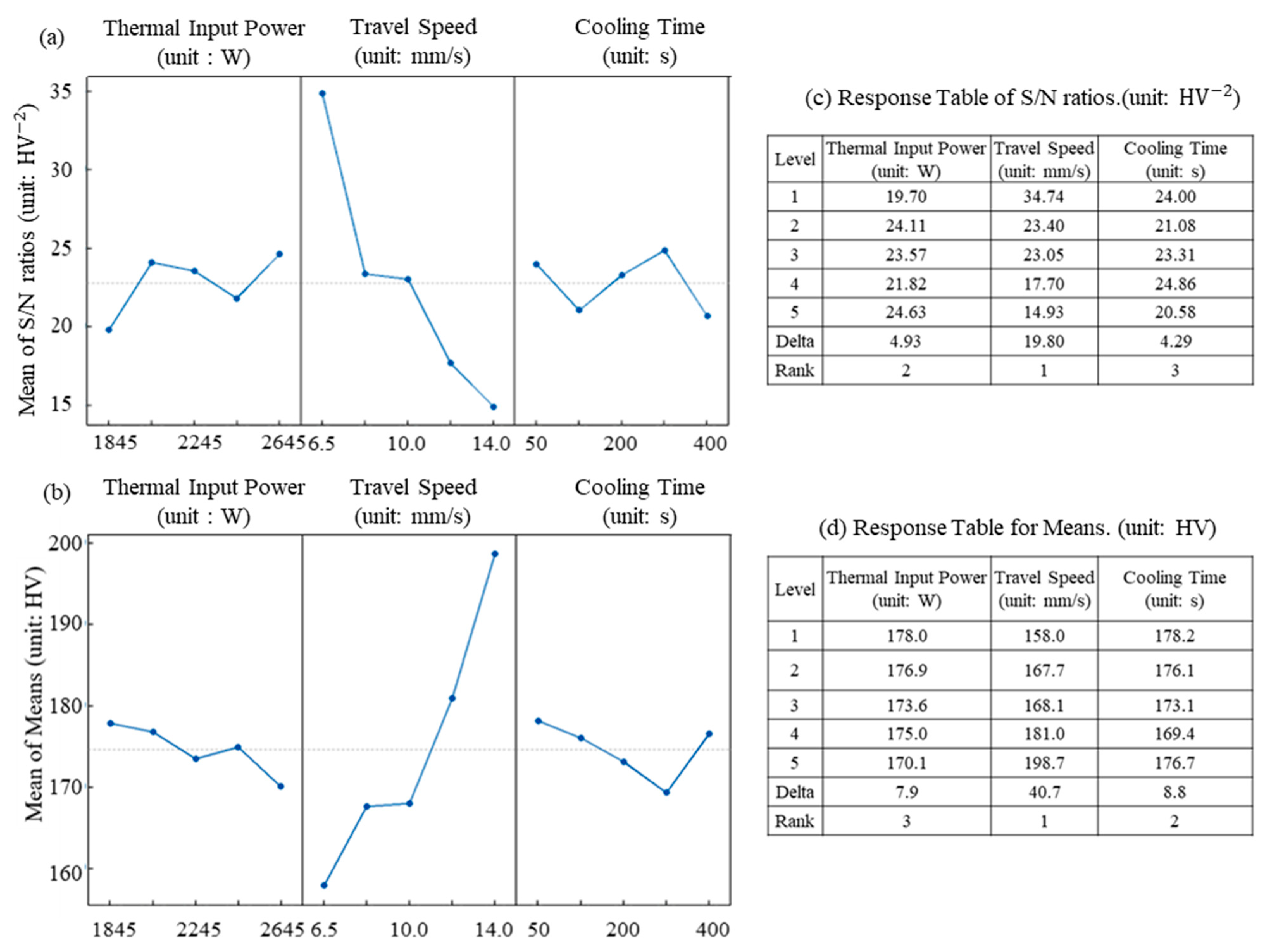
The values of the process parameters used in the simulations and the corresponding hardness results are displayed in Table 2. The signal-to-noise (S/N) ratio and the mean of the simulation results are analyzed and reported in Figure 12c,d respectively. Based on this analysis, it can be concluded that the input parameter with the most significant impact on hardness is the travel speed. Thereafter, both the input energy and cooling time have a similar impact on the hardness.

Figure 12. (a) Signal-to-Noise (S/N) ratio plot; (b) Mean of Means plot; (c) response table of S/N ratios; (d) response table for Means Figure 13 provides the contour plots that illustrate the relation between the process parameters and hardness. The large values of hardness, more specifically those above 240 HV, are the consequence of the martensite phase in the mild steel. To avoid the presence of brittle martensite in the WAAM deposit, the travel speed should be lower than 10 mm/min. This observation aligns with the findings from the contour plots in Figure 13.

Figure 12. (a) Signal-to-Noise (S/N) ratio plot; (b) Mean of Means plot; (c) response table of S/N ratios; (d) response table for Means Figure 13 provides the contour plots that illustrate the relation between the process parameters and hardness. The large values of hardness, more specifically those above 240 HV, are the consequence of the martensite phase in the mild steel. To avoid the presence of brittle martensite in the WAAM deposit, the travel speed should be lower than 10 mm/min. This observation aligns with the findings from the contour plots in Figure 13.

3.4. Analysis of Results Obtained from the ANN Prediction Model

As discussed in Section 2.4, the number of neurons in the hidden layer varied from 3 to 13. The corresponding performance metrics R², RMSE, and MAPE were calculated and are shown in Figure 14. Based on the maximum R and minimum RMSE values, the optimal number of neurons in the hidden layer for determining hardness was determined to be 10. Therefore, the ANN models for HV1, HV2, HV3, and HV4 are developed using a 3-10-1 network architecture unless specified otherwise. The values of the performance metrics are summarized in

Table 6. Performance of the different hardness models.

ANN	${\mathit{R}}^2$	$\mathit{R}\mathit{M}\mathit{S}\mathit{E}$	$\mathit{M}\mathit{A}\mathit{P}\mathit{E}$
HV1	0.9232	0.0239	2.4
HV2	0.9231	0.0235	2.5
HV3	0.9581	0.0203	1.8
HV4	0.9601	0.0179	2.0

.

In this study, back propagation ANNs with the selected architecture were developed. A comparison of the target values and prediction results obtained for HV1, HV2, HV3, and HV4 is shown in Figure 15. In most conditions, the same values are obtained for the targets and predicted results. The maximum relative errors of HV1, HV2, HV3, as well as HV4, are within ±20%. These observations are the first evidence of the ANN model performance. Additionally, the performance is analyzed based on the $R^2$, $RMSE$, and $MAPE$ metrics which are reported in Table 6. The $MAPE$ values for the ANN estimations are 2.4% for HV1, 2.5% for HV2, 1.8% for HV3, and 2.0% for HV4. The results confirm that the ANN yields a high prediction accuracy for hardness for the range of simulated process parameters. In addition, the training of neurons reveals a high correlation for the output parameters HV1, HV2, HV3, and HV4 (Figure 16). Based on the above results, it can be concluded that the ANN model shows a good prediction performance for the studied set of numerical experiments.

4. Conclusions

This manuscript discussed the development of an ANN hardness prediction tool, based on the finite element implementation of a thermal–metallurgical model for mild steel produced by WAAM. The following three main conclusions can be drawn:

• The proposed thermal–metallurgical model for mild steel not only accurately quantifies the heating and cooling cycles during the wire arc additive manufacturing process, but also predicts the complex distribution of microstructural phases and the related hardness for the WAAM component.
• A series of thermal–metallurgical simulations, defined using the Taguchi design of experiments, clearly indicated that travel speed is the most significant process parameter with respect to hardness. Complementary, the input energy and cooling time exhibit noticeable effects on hardness.
• The developed ANN prediction model demonstrates a high accuracy in predicting hardness values.

In future work, the models will be extended towards the prediction of residual stresses that are known to impact fatigue strength.

References

- Javadi, Y.; MacLeod, C.N.; Pierce, S.G.; Gachagan, A.; Lines, D.; Mineo, C.; Ding, J.; Williams, S.; Vasilev, M.; Mohseni, E.; et al. Ultrasonic Phased Array Inspection of a Wire + Arc Additive Manufactured (WAAM) Sample with Intentionally Embedded Defects. Addit. Manuf. 2019, 29, 100806. [Google Scholar] [CrossRef]
- Rodrigues, T.A.; Duarte, V.R.; Tomás, D.; Avila, J.A.; Escobar, J.D.; Rossinyol, E.; Schell, N.; Santos, T.G.; Oliveira, J.P. In-Situ Strengthening of a High Strength Low Alloy Steel during Wire and Arc Additive Manufacturing (WAAM). Addit. Manuf. 2020, 34, 101200. [Google Scholar] [CrossRef]
- Ghaffari, M.; Vahedi Nemani, A.; Nasiri, A. Microstructure and Mechanical Behavior of PH 13–8Mo Martensitic Stainless Steel Fabricated by Wire Arc Additive Manufacturing. Addit. Manuf. 2022, 49, 102374. [Google Scholar] [CrossRef]
- Montevecchi, F.; Venturini, G.; Grossi, N.; Scippa, A.; Campatelli, G. Finite Element Mesh Coarsening for Effective Distortion Prediction in Wire Arc Additive Manufacturing. Addit. Manuf. 2017, 18, 145–155. [Google Scholar] [CrossRef]
- Nijhuis, B.; Geijselaers, H.J.M.; van den Boogaard, A.H. Efficient Thermal Simulation of Large-Scale Metal Additive Manufacturing Using Hot Element Addition. Comput. Struct. 2021, 245, 106463. [Google Scholar] [CrossRef]
- Wu, B.; Ding, D.; Pan, Z.; Cuiuri, D.; Li, H.; Han, J.; Fei, Z. Effects of Heat Accumulation on the Arc Characteristics and Metal Transfer Behavior in Wire Arc Additive Manufacturing of Ti6Al4V. J. Mater. Process. Technol. 2017, 250, 304–312. [Google Scholar] [CrossRef]
- Boruah, D.; Dewagtere, N.; Ahmad, B.; Nunes, R.; Tacq, J.; Zhang, X.; Guo, H.; Verlinde, W.; De Waele, W. Digital Image Correlation for Measuring Full-Field Residual Stresses in Wire and Arc Additive Manufactured Components. Materials 2023, 16, 1702. [Google Scholar] [CrossRef] [PubMed]
- Wu, B.; Pan, Z.; Ding, D.; Cuiuri, D.; Li, H.; Xu, J.; Norrish, J. A Review of the Wire Arc Additive Manufacturing of Metals: Properties, Defects and Quality Improvement. J. Manuf. Process. 2018, 35, 127–139. [Google Scholar] [CrossRef]
- Guo, L.; Zhang, L.; Andersson, J.; Ojo, O. Additive Manufacturing of 18% Nickel Maraging Steels: Defect, Structure and Mechanical Properties: A Review. J. Mater. Sci. Technol. 2022, 120, 227–252. [Google Scholar] [CrossRef]
- Zhang, D.; Liu, A.; Yin, B.; Wen, P. Additive Manufacturing of Duplex Stainless Steels—A Critical Review. J. Manuf. Process. 2022, 73, 496–517. [Google Scholar] [CrossRef]
- Ghafouri, M.; Ahn, J.; Mourujärvi, J.; Björk, T.; Larkiola, J. Finite Element Simulation of Welding Distortions in Ultra-High Strength Steel S960 MC Including Comprehensive Thermal and Solid-State Phase Transformation Models. Eng. Struct. 2020, 219, 110804. [Google Scholar] [CrossRef]
- Mi, G.; Xiong, L.; Wang, C.; Hu, X.; Wei, Y. A Thermal-Metallurgical-Mechanical Model for Laser Welding Q235 Steel. J. Mater. Process. Technol. 2016, 238, 39–48. [Google Scholar] [CrossRef]
- Lusk, M. Martensitic Phase Transitions with Surface Effects. J. Elast. 1994, 34, 191–227. [Google Scholar] [CrossRef]
- Roy, M.; Wodo, O. Data-Driven Modeling of Thermal History in Additive Manufacturing. Addit. Manuf. 2020, 32, 101017. [Google Scholar] [CrossRef]
- Mozaffar, M.; Paul, A.; Al-Bahrani, R.; Wolff, S.; Choudhary, A.; Agrawal, A.; Ehmann, K.; Cao, J. Data-Driven Prediction of the High-Dimensional Thermal History in Directed Energy Deposition Processes via Recurrent Neural Networks. Manuf. Lett. 2018, 18, 35–39. [Google Scholar] [CrossRef]
- Farias, F.W.C.; da Cruz Payão Filho, J.; Moraes e Oliveira, V.H.P. Prediction of the Interpass Temperature of a Wire Arc Additive Manufactured Wall: FEM Simulations and Artificial Neural Network. Addit. Manuf. 2021, 48, 102387. [Google Scholar] [CrossRef]
- Yaseer, A.; Chen, H. Machine Learning Based Layer Roughness Modeling in Robotic Additive Manufacturing. J. Manuf. Process. 2021, 70, 543–552. [Google Scholar] [CrossRef]
- Le, V.T.; Nguyen, H.D.; Bui, M.C.; Pham, T.Q.D.; Le, H.T.; Tran, V.X.; Tran, H.S. Rapid and Accurate Prediction of Temperature Evolution in Wire plus Arc Additive Manufacturing Using Feedforward Neural Network. Manuf. Lett. 2022, 32, 28–31. [Google Scholar] [CrossRef]
- Pant, P.; Chatterjee, D. Prediction of Clad Characteristics Using ANN and Combined PSO-ANN Algorithms in Laser Metal Deposition Process. Surf. Interfaces 2020, 21, 100699. [Google Scholar] [CrossRef]
- Xia, C.; Pan, Z.; Polden, J.; Li, H.; Xu, Y.; Chen, S. Modelling and Prediction of Surface Roughness in Wire Arc Additive Manufacturing Using Machine Learning. J. Intell. Manuf. 2022, 33, 1467–1482. [Google Scholar] [CrossRef]
- Ding, J.; Colegrove, P.; Mehnen, J.; Ganguly, S.; Almeida, P.M.S.; Wang, F.; Williams, S. Thermo-Mechanical Analysis of Wire and Arc Additive Layer Manufacturing Process on Large Multi-Layer Parts. Comput. Mater. Sci. 2011, 50, 3315–3322. [Google Scholar] [CrossRef]
- Ding, D.; Zhang, S.; Lu, Q.; Pan, Z.; Li, H.; Wang, K. The Well-Distributed Volumetric Heat Source Model for Numerical Simulation of Wire Arc Additive Manufacturing Process. Mater. Today Commun. 2021, 27, 102430. [Google Scholar] [CrossRef]
- Goldak, J.; Chakravarti, A.; Bibby, M. A New Finite Element Model for Welding Heat Sources. Metall. Trans. B. 1984, 15, 299–305. [Google Scholar] [CrossRef]
- Eagar, T.W.; Tsai, N.S. Temperature Fields Produced By Traveling Distributed Heat Sources. Weld. J. 1983, 62, 346–355. [Google Scholar]
- Ai, Y.; Liu, X.; Huang, Y.; Yu, L. Numerical Analysis of the Influence of Molten Pool Instability on the Weld Formation during the High Speed Fiber Laser Welding. Int. J. Heat Mass Transf. 2020, 160, 120103. [Google Scholar] [CrossRef]
- Ai, Y.; Yu, L.; Huang, Y.; Liu, X. The Investigation of Molten Pool Dynamic Behaviors during the “∞” Shaped Oscillating Laser Welding of Aluminum Alloy. Int. J. Therm. Sci. 2022, 173, 107350. [Google Scholar] [CrossRef]
- Chiumenti, M.; Cervera, M.; Salmi, A.; Agelet de Saracibar, C.; Dialami, N.; Matsui, K. Finite Element Modeling of Multi-Pass Welding and Shaped Metal Deposition Processes. Comput. Methods Appl. Mech. Eng. 2010, 199, 2343–2359. [Google Scholar] [CrossRef]
- Lindgren, L.E.; Hedblom, E. Modelling of Addition of Filler Material in Large Deformation Analysis of Multipass Welding. Commun. Numer. Methods Eng. 2001, 17, 647–657. [Google Scholar] [CrossRef]
- Trzaska, J.; Dobrzański, L.A. Modelling of CCT Diagrams for Engineering and Constructional Steels. J. Mater. Process. Technol. 2007, 192–193, 504–510. [Google Scholar] [CrossRef]
- Kakhki, M.E.; Kermanpur, A.; Golozar, M.A. Numerical Simulation of Continuous Cooling of a Low Alloy Steel to Predict Microstructure and Hardness. Model. Simul. Mater. Sci. Eng. 2009, 17, 045007. [Google Scholar] [CrossRef]
- Maynier, P.; Dollet, J.; Bastien, P. Prediction of Microstructure via Empirical Formulae Based on Cct Diagrams; Metallurgical Society AIME: San Ramon, CA, USA, 1978; pp. 163–178. [Google Scholar]
- Pradeep Kumar, J.; Jaanaki Raman, R.; Jerome Festus, N.; Kanmani, M.; Praveen Nath, S. Optimization of Wire Arc Additive Manufacturing Parameters Using Taguchi Grey Relation Analysis. In Proceedings of the 2023 International Conference on Intelligent Systems for Communication, IoT and Security (ICISCoIS), Coimbatore, India, 9–11 February 2023; pp. 108–113. [Google Scholar] [CrossRef]
- Taguchi, G.; Yokoyama, Y.; Wu, Y. Taguchi Methods: Design of Experiments; ASI Press: Okhotsk, Japan, 1993. [Google Scholar]
- Denlinger, E.R.; Irwin, J.; Michaleris, P. Thermomechanical Modeling of Additive Manufacturing Large Parts. J. Manuf. Sci. Eng. Trans. ASME 2014, 136, 061007. [Google Scholar] [CrossRef]
- Yu, F.; Wei, Y. Phase-Field Investigation of Dendrite Growth in the Molten Pool with the Deflection of Solid/Liquid Interface. Comput. Mater. Sci. 2019, 169, 109128. [Google Scholar] [CrossRef]
Figure 1.
Proposed simulation framework to build the ANN-based thermal–metallurgical model: illustrations of (a) Temperature distribution; (b) Ferrite distribution; (c) Hardness distribution; (d) Correlation of the predicted values versus target values.
Figure 2.
(a) Heat distribution over a double-ellipsoidal space (Reprinted with permission from Ref. [23]. 2024 Springer Nature BV); (b) Well-distributed volumetric heat source (orange block) and an illustration of the grid element activation for the WAAM process; (c) Heat distribution over a Gaussian space (Reprinted from Ref. [22]).
Figure 3.
Geometry of the WAAM component, and identification of the positions TPx of the thermocouples used in the experiments of the work presented in (Reprinted with permission from Ref. [21]. 2024 Elsevier), as well as the locations for which hardness is numerically determined.
Figure 4.
Mesh of the finite element model used for thermal simulations. (Note that the different heat source models implemented in this study used the same mesh model).
Figure 5.
Flowchart of the procedure applied for the simulation of multiphase transformation kinetics.
Figure 6.
Single output ANN model—back propagation structure.
Figure 7.
Comparison of the temperature–time curves for the three mesh configurations with experimental values.
Figure 8.
(a–d) Comparison of the experimental (Reprinted with permission from Ref. [21]. 2024 Elsevier) and numerical temperature history results for three different heat source models; (e) relative errors of the temperature history results of the well-distributed volumetric heat source model compared to the experimental results.
Figure 9.
Temperature distribution from: (a) publication (Reprinted with permission from Ref. [21]. 2024 Elsevier); (b) the well-distributed heat source model; (c) the Gaussian heat source model; (d) the double-ellipsoid heat source model.
Figure 10.
(a–f) Thermal cycle curves at points A, B, C, D, in the deposit, and points S1 and S0 in the substrate.
Figure 11.
Distribution of the (a–e) phases at the mid-section: ferrite, pearlite, bainite, austenite, martensite; and (f) hardness.
Figure 13.
Contour plots of the hardness () vs. (a) travel speed (TS) and cooling time (CL); and (b) travel speed (TS) and thermal input power (Q).
Figure 14.
Values of (a) , (b) root mean square error for different numbers of neurons in the ANN models for hardness prediction.
Figure 15.
Target values and ANN predicted values of (a) HV1, (b) HV2, (c) HV3, (d) HV4.
Figure 16.
Correlation of the ANN predicted values versus data from the numerical experiments for (a) HV1 (position A); (b) HV2 (position B); (c) HV3 (position C) and (d) HV4 (position D).