Research on the Identification of Nonlinear Wheel–Rail Adhesion Characteristics Model Parameters in Electric Traction System Based on the Improved TLBO Algorithm

Abstract

The wheel–rail adhesion is one of the key factors limiting the traction performance of railway vehicles. To meet the adhesion optimization needs and rapidly obtain wheel–rail creep characteristics under specific operating conditions, an engineering identification method for wheel–rail adhesion characteristics based on a nonlinear model is proposed. The proposed method, built upon the traditional Teaching-Learning-Based Optimization (TLBO) algorithm, has been adapted to the specific nature of nonlinear wheel–rail adhesion model parameters identification, enhancing both the search speed in the early stages and the search accuracy in the later stages of the algorithm. The proposed identification algorithm is validated using experimental data from the South African 22E dual-flow locomotive. The validation results demonstrate that the proposed identification algorithm can obtain a nonlinear wheel–rail adhesion characteristics model with an average adhesion coefficient error of around 0.01 within 50 iteration steps. These validation results indicate promising prospects for the engineering practice of the proposed algorithm.

1. Introduction

Rail traffic is among the most efficient and lowest-emitting modes of transport, which reduces greenhouse gas emissions, air pollution, and congestion [1,2,3]. To satisfy the requirement of rail traffic expansion, railway vehicles with higher speed and greater transportation capacity are urgently needed. Therefore, it has become inevitably necessary to improve the unit traction power of railway vehicles.

However, the wheel–rail contact limits the traction and braking capabilities of railway vehicles, although it can significantly reduce the running resistance of the train. When the traction torque exerted on the driven wheel exceeds the physical adhesion limit of the wheel–rail contact, the wheel slippage phenomenon occurs, which leads to the damage of wheel and rail in a serious situation [4]. Therefore, wheel–rail adhesion utilization is one of the most important factors influencing the actual traction power of railway vehicles. Generally, there are two ways to improve the utilization performance of wheel–rail adhesion. One is to assemble the sanders, which improves the adhesion conditions by the application of sand into the wheel–rail contact [5]. The other is to employ the adhesion utilization control, which makes better use of the available adhesion in the wheel–rail contact by operating at optimal creep status [6]. However, the sanding increases 10 to 100 times the wheel and rail wear, which makes the adhesion utilization control more preferred.

With the rapid development of electric traction control, several adhesion utilization control algorithms have been proposed to improve the adhesion utilization performance of railway vehicle in recent years, such as re-adhesion control [7,8] and slip control [6,9,10,11,12]. The former limits the slip velocity to an acceptable value after the slip phenomenon has already occurred, while the latter controls the slip velocity in a proper range around the maximum value of the adhesion–slip characteristic. As a result, the slip control can prevent the slip phenomenon by continuous slip velocity adjustment. To achieve optimal adhesion utilization, accurate information of the maximum adhesion–slip point is a necessary condition for realizing slip control. Therefore, the core of the slip controllers based on maximum point detection is identifying the maximum point on the adhesion–slip characteristic.

In the early years, the slip velocity of the maximum point was set to a constant value measured in previous trials, which assumes the maximum value of the adhesion coefficient occurs approximately at the same slip velocity [11]. In fact, the adhesion–slip characteristic has been changing during train operation, especially, the characteristic differs between dry, wet, and icy rail. As a result, the constant value was difficult to satisfy the requirement of maximum adhesion utilization. To estimate the accurate information of wheel–rail adhesion–slip characteristic, many adhesion identification approaches have been proposed [13], which can be classified into data-driven methods and theoretical model-based methods.

The data-driven identification methods typically use data-based models, such as empirical formula model [14], artificial neural network model [15], Kalman filter-based identification model [9], or machine learning-based model [16], to identify the adhesion characteristic. However, the accuracy of data-driven models depended on the coverage of the training data samples. In engineering applications, once the wheel–rail adhesion conditions change beyond the coverage of the initial training samples, it is easy to identify irregular adhesion characteristic curves. On the contrary, the theoretical model-based methods, which utilized the theory of creep to establish mathematical relationships between wheel–rail adhesion characteristic and vehicle state parameters, can confine the identified adhesion characteristic curves within regular curves [17]. The challenge of the theoretical model-based methods is to establish a theoretical model that can exactly describe the wheel–rail adhesion characteristics under various conditions, and to accurately identify the model parameters online [18].

The research on the wheel–rail creep theoretical model has a long history, including Carter’s two-dimensional rolling contact creep theory, V-J no-spin three-dimensional rolling contact model, Shen’s improved small-spin three-dimensional rolling contact model, the Kalker precise creep theory (abbreviated as CONTACT), and the Kalker Simplified Theory (abbreviated as FASTSIM) [19]. The above models employed a constant friction coefficient, resulting in discrepancies between the calculated adhesion characteristic curves and experimental measurements, particularly after reaching the maximum adhesion coefficient. In addition, swarm intelligence-based multiple models approach is proposed in Ref. [20], which is promising to be used as an on-board friction condition monitoring tool for railway vehicles with traction. A real-time estimation of the wheel–rail contact forces based on an estimator design model that takes into account the nonlinearities of the interaction by means of a fitting model functional to reproduce the contact mechanics in a wide range of slip, and is easily integrated in a complete model-based estimator for railway vehicles [21]. Suitable modelling of the railway vehicle dynamics is presented in Ref. [22] for the model-based estimator synthesis to perform the equivalent conicity monitoring employing only the carbody and bogie frame measurements, taking into account the track adhesion level variation. Ref. [23] presents a particle swarm optimization (PSO)-based Extended Kalman Filter (EKF) to estimate adhesion force. A new approach, based on FASTSIM algorithm and Polach theory, is numerically very efficient and has been specifically designed for an innovative degraded adhesion model [24]. In Ref. [25], a finite element model is developed to investigate the mechanical behavior of sand particles in a wheel–rail contact and how they affect the adhesion level. Ref. [26] proposed a three-dimensional wheel–rail adhesion model under wet conditions, which considers insufficient water supply, the measured surface roughness, and dynamic effect of the vehicle and track system.

Among the aforementioned influencing factors of adhesion coefficient, the wheel slip velocity, which is defined as the difference between a wheel circumference velocity and the vehicle longitudinal velocity, is the most suitable and adjustable factor for adhesion utilization [27,28,29]. As shown in Figure 1, there is a nonlinear relationship, which is usually called adhesion–slip characteristic, between wheel slip and adhesion coefficient. Regardless of wheel–rail contact conditions, there is always a peak point, which is also known as the maximum adhesion point, on the adhesion–slip curve. The slip corresponding to the maximum adhesion point is the optimal slip. The area on the left side of the maximum adhesion point is called the stable zone, in which the adhesion coefficient increases with wheel slip.

To better simulate wheel–rail adhesion characteristics, Polach [30] proposed a novel wheel–rail creep model based on FASTSIM, which incorporated a friction coefficient that varies with creep speed and includes a damping factor. Additionally, it utilized an adhesion/slip zone adjustment coefficient when calculating wheel–rail creep forces. As a result, it achieved a high degree of agreement with experimental data. Considering the engineering reliability and universality, FASTSIM will be studied in this paper due to its wide implementation in engineering cases and simulation software.

However, fitting examples provided by Polach and other scholars indicated significant variations in parameter configurations of the Polach’s wheel–rail creep model due to factors such as vehicle type, speed category, and track conditions [31,32,33,34]. Therefore, relying solely on characteristic parameters of the Polach’s creep model under typical track conditions cannot meet the adhesion optimal utilization control requirements of engineering practice. However, when fitting specific wheel–rail adhesion characteristics, it is necessary to adjust numerous model parameters in the Polach’s creep model, many of which lack clear physical significance [35,36]. It is difficult to achieve globally optimal model parameters using traditional parameter identification methods.

To enhance the efficiency of wheel–rail adhesion characteristic identification and meet the practical engineering application requirements, an engineering-oriented identification method for wheel–rail adhesion characteristics based on the Polach’s creep model is proposed in this paper. The proposed method not only enables the real-time observation of adhesion coefficients using existing traction system state information, but also allows rapid acquisition of the corresponding Polach’s model parameters, thus obtaining comprehensive information of wheel–rail adhesion–slip characteristics. For accurate identification of model parameters, a swarm intelligence search method is introduced. To enhance identification accuracy and convergence speed, the characteristics of the Polach’s model are considered and targeted improvements are made to the original Teaching-Learning-Based Optimization (TLBO) algorithm. Those improvements enable adaptive adjustment of the model parameter search gradient and enhance both the early-stage search speed and the late-stage search accuracy of the proposed algorithm.

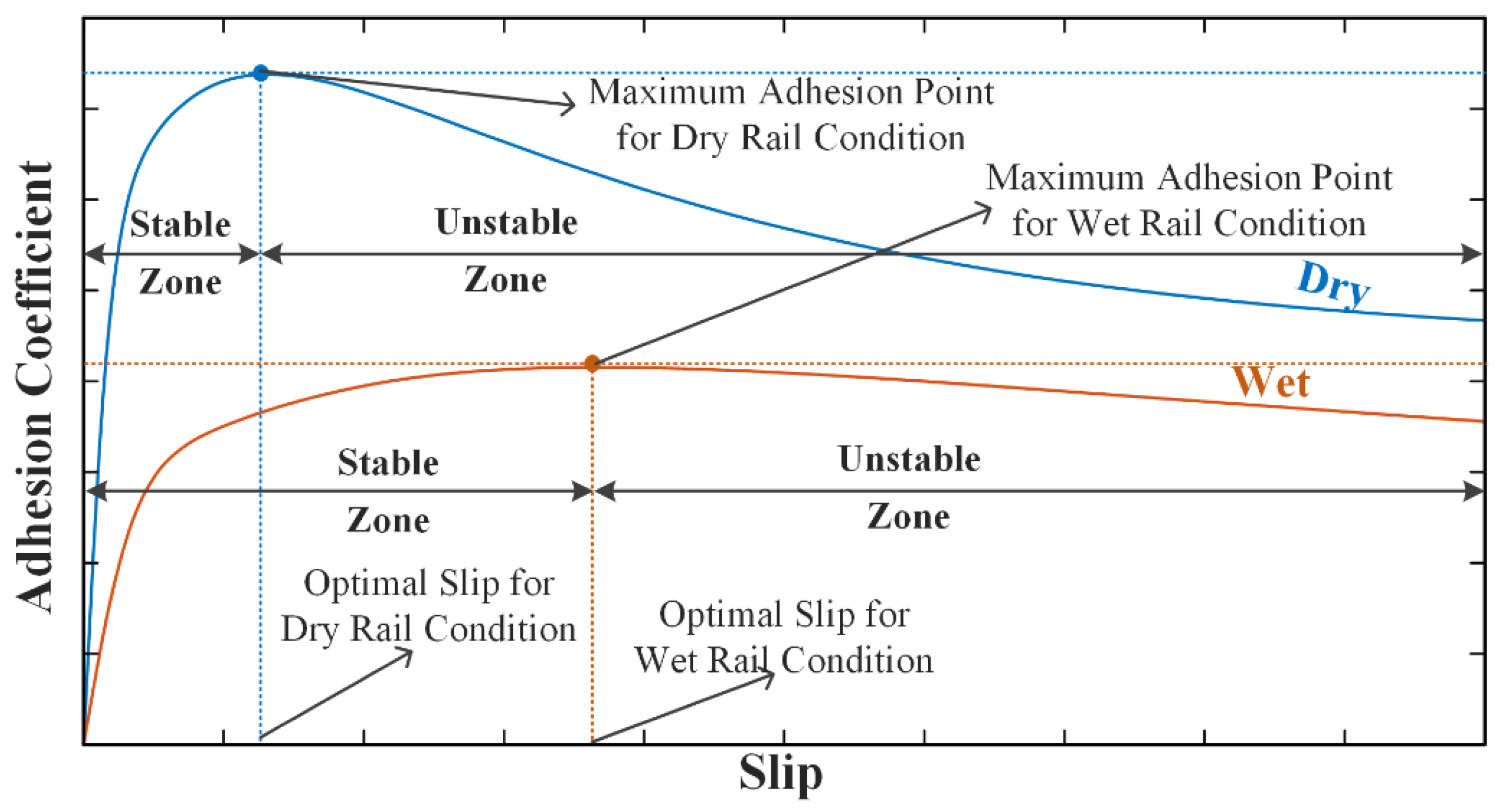
2. Nonlinear Model of Wheel–Rail Adhesion Characteristics

To numerically simulate the adhesion characteristics between wheel–rail contact, the model of Polach has been implemented in this study [30]. The Polach’s method assumes that the maximum tangential stress ${\tau }_{\max }$ distribution on wheel–rail contact satisfies Coulomb’s friction law:

$${\tau }_{\max }=\mu \cdot \sigma$$

(1)

where $\mu$ is friction coefficient of wheel–rail contact, and $\sigma$ is normal stress on the wheel–rail contact surface.

In addition, according to the Hertz theory, the Polach’s method assumes that the contact spot of wheel–rail is an ellipse, and semi-axis length of the ellipse can be calculated by Hertz theory according to the axle weight and wheel–rail size. The slip area, adhesion area, and tangential/normal stress distribution in the elliptical contact spot are shown in Figure 2, and the maximum normal stress can be calculated using:

$${\sigma }_0=\frac{3}{2}\frac{Q}{\pi ab}$$

(2)

where $Q$ is the normal force exerted on wheel–rail contact, which is also called wheel load, and $a$ and $b$ are the semi-axis lengths of the elliptical contact spot.

The relative displacement between the wheel and rail in wheel–rail contact increases linearly from point A to point C. In the adhesion area (i.e., A-B), the relative displacement between the wheel and rail is caused by the deformation of the material, and the tangential stress of wheel–rail increases linearly simultaneously. If the tangential stress $\tau$ reaches its maximum value ${\tau }_{\max }$ in the trailing point (B) of adhesion area, a slip motion of the wheel–rail contact surface appears. Hence, the area from point B to point A is called the slip area. According to the Kalker’s simplified theory, assuming that the tangential stress is proportional to the slip $s$ and the distance from the leading point A with proportionality constant $C$, which is the tangential contact stiffness of the wheel–rail contact surface. Then, the gradient of tangential stress $\epsilon$ in adhesion area of wheel–rail contact surface is:

$$\epsilon =\frac{2}{3}\frac{C\pi a^{2}b}{Q\cdot \mu }s$$

(3)

where $s=v_s/v_v$ is the slip ratio between the wheel and rail, $v_s$ is the wheel slip velocity, and $v_v$ is the train velocity.

The total adhesion force $F_{adh}$ of wheel–rail contact can be obtained by integrating the tangential stress in the elliptical contact spot:

$$F_{adh}={\displaystyle \underset{U}{\iint }\tau \mathrm{d}x\mathrm{d}y}$$

(4)

where $U$ is the contact area of wheel–rail, and $\tau$ is the tangential stress in wheel–rail contact.

To solve Equation (4), the tangential force distribution is transformed from an ellipsoid to a hemisphere by the coordinate transformation shown in Figure 3. Finally, the total adhesion force is obtained as:

$$F_{adh}=-\frac{2Q\mu }{\pi }(\frac{\epsilon }{1+{\epsilon }^2}+\arctan \epsilon )$$

(5)

Considering the phenomenon of the friction coefficient decreases with increasing wheel slip, a variable friction coefficient was proposed by Polach:

$$\mu ={\mu }_0\left[\left(1-A\right)e^{-B{v}_s}+A\right]$$

(6)

where $A={\mu }_{\infty }/{\mu }_0$ is the ratio of limit friction coefficient at infinity wheel slip ${\mu }_{\infty }$ to the maximum friction coefficient ${\mu }_0$, and $v_s$ is the slip velocity.

Since the contaminants between wheel and rail contact decreases the stiffness of the contact surface, the adhesion force–slip function reduces its gradient significantly. To model the adhesion degradation of wheel–rail contact under contaminants, Equation (5) has been modified by Polach as:

$$F_{adh}=\frac{2Q\mu }{\pi }\left(\frac{k_A\epsilon }{1+{\left(k_A\epsilon \right)}^2}+\arctan \left(k_S\epsilon \right)\right), k_S\le k_A\le 1$$

(7)

where $k_A$ is the reduction factor in the adhesion area, and $k_S$ is the adjustment factor in the slip area.

According to Equation (7), the numerical model of adhesion coefficient ${\mu }_{adh}$ can be given as:

$${\mu }_{adh}=\frac{2\mu }{\pi }\left(\frac{k_A\epsilon }{1+{\left(k_A\epsilon \right)}^2}+\arctan \left(k_S\epsilon \right)\right), k_S\le k_A\le 1$$

(8)

3. Wheel–Rail Adhesion Characteristics Model Parameters Identification Approach

This section began with a brief introduction to the basic principles of the Teaching-Learning-Based Optimization (TLBO) algorithm, followed by a detailed presentation of the proposed wheel–rail adhesion characteristic identification algorithm based on Polach’s model, along with its engineering implementation methodology.

3.1. Teaching-Learning-Based Optimization Methodology

TLBO algorithm, also known as ‘teaching and learning’, was first introduced by Professor R.V. RAO in 2011 [37]. It is a novel swarm intelligence search algorithm similar to Particle Swarm Optimization (PSO). With its advantages of fast convergence, strong adaptability, and search precision independent of parameter settings, TLBO has been widely applied in various fields within just a few years [38,39,40]. The inspiration for the TLBO algorithm is derived from classroom teaching activities, where the feasible solution set for problem-solving was abstracted as a ‘student’ population. The objective function values corresponding to each set of solutions were abstracted as students’ grades, and the iterative search process is divided into two phases: teacher and student.

3.1.1. Teacher Phase

The teaching process by the teacher is illustrated in Figure 4. Before the teacher imparts knowledge to the students, the teacher possesses the highest level of understanding of the course. Therefore, the best-performing ‘student’ individual, which represents the best solution of the current iteration, is selected as the ‘teacher’ (marked as $T_{\mathrm{i}}$) for this stage. According to the level of mastery of the course, the grades of the ‘students’ in the class vary greatly. Aiming to improve the overall class average grade, the “teacher” designs the teaching content based on the difference between the class average performance and its own performance. If the average grade of the class at the i-th iteration step is denoted as $M_{\mathrm{i}}$, then the teaching content of the teacher for the j-th student at the i-th iteration step could be expressed by the following equation:

$$X_{\mathrm{diff},j}=r_j\left(T_i-T_F{M}_i\right); j=1,2,\cdots ,class\_size$$

(9)

where $r_j$ is a random number in the range [0, 1], representing the learning ability of the student; $T_F=round[1+rand(0,1)]$ is the teaching coefficient for this phase, which is used to simulate the teacher’s teaching ability; $class\_size$ is the class size, i.e., the population size. After completing the teacher’s teaching process, the student who has received new knowledge can be represented by:

$$X_{\mathrm{new},j}=X_{\mathrm{old},j}+X_{\mathrm{diff},j}$$

(10)

If $X_{\mathrm{new},j}$ is better than $X_{\mathrm{old},j}$, replace $X_{\mathrm{new},j}$ with $X_{\mathrm{old},j}$; otherwise, retain $X_{\mathrm{old},j}$.

3.1.2. Learner Phase

In addition to learning from the teacher, students can also improve their grades by engaging in peer-to-peer exchanges. For each student $X_j$, another classmate $X_k$ can be selected from the class. The two students can engage in mutual learning by comparing their grades with each other:

$$\left\{\begin{array}{cc}{X}_{new,j}=X_{old,j}+r_j(X_j-X_k)& \mathrm{if} f(X_j)<f(X_k)\\ X_{new,j}=X_{old,j}+r_j(X_k-X_j)& \mathrm{if} f(X_j)\ge f(X_k)\end{array}\right.$$

(11)

If $X_{\mathrm{new},j}$ is better than $X_{\mathrm{old},j}$, replace $X_{\mathrm{new},j}$ with $X_{\mathrm{old},j}$; otherwise, retain $X_{\mathrm{old},j}$.

3.2. An Improved TLBO Algorithm for Wheel–Rail Adhesion Characteristic Identification

As described in the previous section, the teacher phase aims to improve the class’s average grade, essentially guiding the population toward the current global optimal solution, which determines the algorithm’s search speed. The learner phase utilized mutual learning among the population to ensure search diversity and prevent convergence to a local optimal. The purpose of employing the TLBO algorithm in this study is to identify wheel–rail adhesion characteristics based on onboard signals. Considering that minor parameter adjustment has little effect on the slip-adhesion curve of the Polach’s model, random changes in wheel–rail conditions would dynamically and significantly affect the parameters of the Polach’s model. Therefore, when utilizing the TLBO algorithm for the identification of wheel–rail adhesion characteristic parameters, corresponding improvements are required to enhance the algorithm’s search breadth and convergence speed.

From the prototype TLBO algorithm, it can be observed that the teaching coefficient in the teacher phase can only take values of 1 and 2. This not only reduces the precision of the search, but also affects the convergence speed. To address this problem, an adaptive teaching coefficient is introduced in this paper:

$$T_F=\frac{M_{i,D}}{T_{i,D}}$$

(12)

where $D=1,2,\cdots D_n$ represents the dimension of the optimization parameters. In Equation (12), the teaching coefficient varies with the difference between the class’s average level and the teacher’s level, thereby achieving adaptive adjustment of the weight between search precision and convergence speed during the search process.

In order to quickly eliminate poorer solutions, this paper introduces a remedial session phase for underperforming students following the learner phase. In this phase, both teacher tutoring and student self-study operations are performed on the bottom 20% of students based on class rankings:

$${\stackrel{⌢}{X}}_{new}=X_{old}+\left[0.5+rand\left(0,1\right)/2\right](T_i-X_{old})$$

(13)

$${\tilde{X}}_{new}=X_{old}+X_{\lim }\times \left[rand\left(0,1\right)-0.5\right]$$

(14)

where ${\stackrel{⌢}{X}}_{new}$ represented the knowledge level of students after teacher tutoring, and this operation aimed to accelerate the convergence speed of the search; ${\tilde{X}}_{new}$ represented the knowledge level of students after self-study, and this operation aimed to enhance the search breadth of the algorithm; $X_{\lim }$ represented the optimization of the search interval size, i.e., the difference between the upper and lower search limits of the optimization parameters. Finally, the optimal solution among $X_{old}$, ${\tilde{X}}_{new}$, and ${\stackrel{⌢}{X}}_{new}$ is retained as the knowledge level of students after remedial session phase.

3.3. Design of the Fitness Function for Identification

According to the characteristics of the Polach’s creep model, $k_A$, $k_s$, $A$, $B$, and ${\mu }_0$ are selected as the optimization parameters for the improved TLBO, with a search parameter dimension $D_n$ of 5. The following objective function is designed to evaluate the fitness of the solution set:

$$fitness=\frac{1}{N}{\displaystyle \sum _{i=1}^N\left|Polach\left(k_A,k_S,A,B,{\mu }_0,v_{s,i},v_{c,i}\right)-{\widehat{\mu }}_{a,i}\right|}$$

(15)

where $N$ is the length of the measured data sequence; $v_{s,i}$ is the wheel slip velocity of the $i$-th measured data point; $v_{c,i}$ is the vehicle speed at the $i$-th measured data point; and ${\widehat{\mu }}_{a,i}$ is the observed adhesion coefficient at the $i$-th measured data point.

However, the actual adhesion coefficient between the wheel and rail of rail vehicles is difficult to directly measure through sensors. In order to observe the wheel–rail adhesion coefficient from the measurement data of onboard sensors, a disturbance observer based on a kinematic model is employed in this paper. According to theoretical mechanics, the relationship between wheelset velocity and traction/braking forces, as well as the actual adhesion force, can be expressed as follows:

$$J\frac{{\dot{v}}_w}{r_w}=T_{\mathrm{T}}-T_{adh}$$

(16)

where $J$ is the wheelset moment of inertia; $v_w$ is the wheelset linear velocity; $r_w$ is the rolling circle radius of the wheelset; $T_{\mathrm{T}}$ is the traction/braking force; $T_{adh}={\mu }_{a}Qg{r}_w$ is the actual adhesion force, where ${\mu }_a$ represents the adhesion coefficient between the wheel and rail.

Taking the Laplace transform of Equation (16) gives:

$$T_{adh}\left(s\right)=T_{\mathrm{T}}\left(s\right)-sJ\frac{V_w\left(s\right)}{r_w}$$

(17)

To reduce the interference introduced by the differential operation in the observer, a first-order low-pass filter is applied to the differential term as follows:

$$s=\left(1/T_0\right)\cdot \left(1-1/\left(1+s{T}_0\right)\right)$$

(18)

By combining Equations (16)–(18), the adhesion coefficient observer is obtained as follows:

$${\widehat{\mu }}_a=\left(T_T-\left(1/T_0\right)\cdot \left(1-1/\left(1+s{T}_0\right)\right)\cdot J\cdot V_w\right)/\left(Q\cdot r_w\right)$$

(19)

where $T_0$ is the time constant of the observer.

3.4. Model-Based Engineering Identification Method for Wheel–Rail Adhesion Characteristics

Based on the principles described above, the design of the wheel–rail adhesion characteristics identification algorithm is illustrated in Figure 5. The algorithm initially generates an initial set of solutions randomly within the search domain. By utilizing Equation (19), the observed adhesion coefficient values are generated as a fitting dataset for the Polach’s model based on the input measured data sequence. The wheel–rail adhesion characteristics corresponding to the parameters of the solution set are simulated by Equations (3), (6) and (8). The fitness of the initial solution set is then evaluated through Equation (15). Subsequently, the algorithm enters an iterative loop of the ‘teacher phase’, ‘learner phase’, and ‘remedial session phase’, continuing until the termination condition is met. Finally, the model-based identification of wheel–rail adhesion characteristics is completed, and the optimized Polach’s model parameters obtained during the search are outputted.

4. Algorithm Verification and Results Discussion

To validate the effectiveness of the proposed algorithm, the identification experiments using measured data from different rail conditions are conducted in this section. Based on the results of identification experiments, a comparative analysis of the identification efficiency and accuracy between the proposed algorithm and other conventional methods is performed.

4.1. Experimental Design for Algorithm Verification

To validate the proposed model-based wheel–rail adhesion characteristic identification algorithm, experiments were conducted to identify the adhesion characteristics of the South African 22E dual-mode locomotive under the scenarios of dry rails, wet rails without sanding, and wet rails with sanding. The South African 22E locomotive adopts a C0-C0 bogie structure with an axle load of 21.5 tons and a new wheel diameter of 1220 mm (semi-worn: 1180 mm, fully worn: 1140 mm). In addition, the South African 22E locomotive can provide a starting traction force of 480 kN and a continuous traction force of 405 kN. Detailed parameters of the adopted locomotive are shown in

Table 1. Parameters of adopted locomotive.

Parameters	Values	Parameters	Values
Supply power	AC 25 kV/50 Hz and DC 3000 V	Maximum operating speed	100 km/m
Axle arrangement	C0-C0	Maximum test speed	110 km/h
Rail gauge	1065 mm	Continuous speed	40 km/m
Total weight	129 t	Starting traction force	480 kN
Axle load	21.5 t	Continuous traction force	405 kN
Wheel diameter	1220 mm (new) 1180 mm (Semi wear) 1140 mm (Wear)	Maximum braking force	300 kN
Continuous output power	4500 kW	Transmission ratio	6.0588

.

In consideration of the primary goal of the experiment, which is to validate the adhesion characteristic identification algorithm, the adhesion identification module does not participate in the implementation of vehicle traction control. Hence, as shown in Figure 6, the adhesion characteristic identification part is independent of the vehicle traction control. The input data for the adhesion characteristic identification module are derived from onboard sensors. Specifically, the wheelset velocity is obtained from the speed sensors, the wheel slip velocity is synthesized by the traction control unit (TCU), and the torque signal is observed by the TCU through motor current and speed signals. The output result of the adhesion characteristic identification module is the model parameters of the Polach’s model. In addition, only the adhesion characteristics of the first wheelset is identified in this paper, for two reasons: (1) all the wheelsets of the locomotive pass through the same rail surface successively, and there is no significant difference in the wheel rail contact surface situation; (2) the rolling of the wheelset has a certain cleaning effect on the rail surface. Hence, the adhesion conditions of the following wheelsets are slightly better than those of the first wheelset.

4.2. Results Discussion and Performance Comparison

To validate the algorithm developed in this paper, this subsection will compare the results of the performance of the particle swarm optimization (PSO) algorithm, the original TLBO algorithm, and the proposed algorithm for wheel–rail adhesion characteristic identification. Due to the suboptimal performance of the PSO algorithm in wheel–rail adhesion characteristic identification, it was introduced only in the dry rails scenario for comparative purposes.

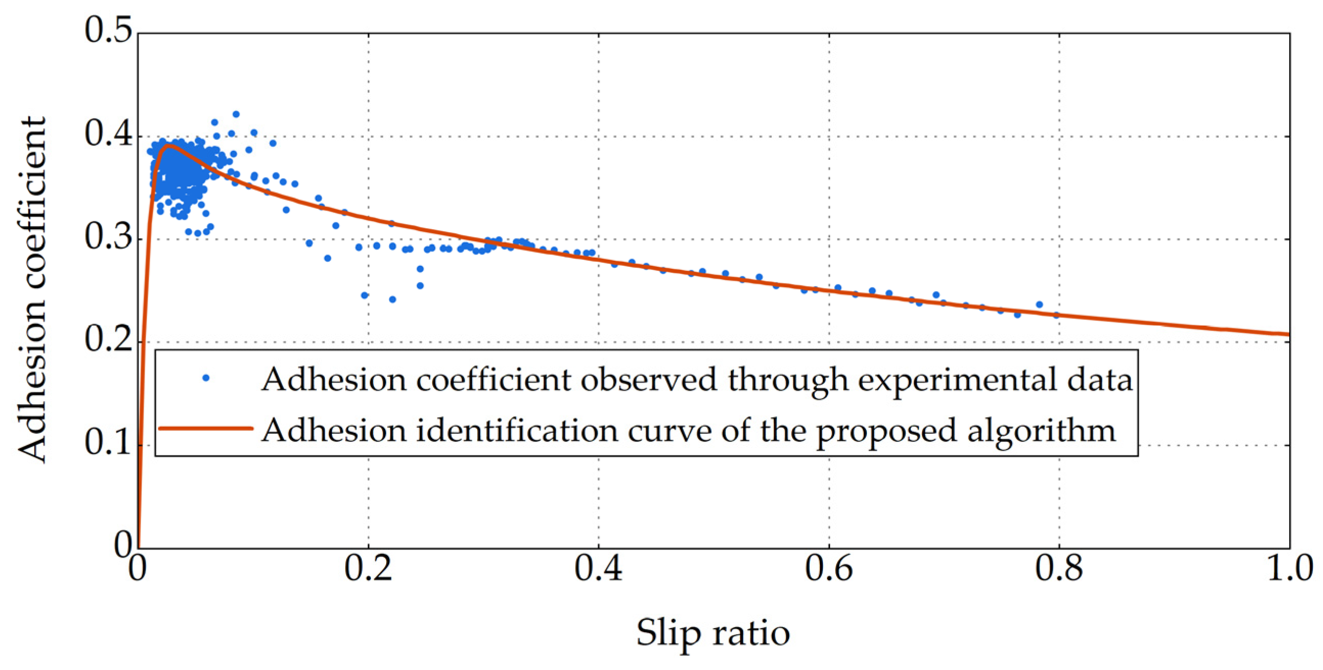
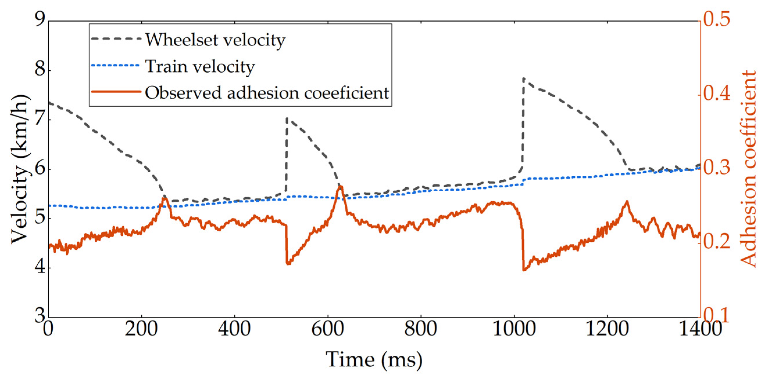
4.2.1. Scenario 1: Dry Rail

A traction acceleration test is conducted on a 22E locomotive in this test scenario, under a dry and straight track surface. Actual traction torque, wheel axle speed, locomotive speed, and other vehicle operational data are collected through the TCU. As shown in Figure 7, the locomotive operates in traction acceleration condition, with an average speed of about 2.2 km/h and a maximum creep speed of 1.65 km/h (corresponding to a real-time creep rate of about 0.8). The distribution range of the adhesion coefficient observed online during the test is [0.23, 0.42], with an average adhesion coefficient of about 0.36, and more than 90% of the adhesion coefficient is distributed in the range above 0.33.

The adhesion coefficient distribution of the 22E locomotive under dry rail conditions is obtained using the adhesion coefficient observer designed in this paper, as illustrated in Figure 8. Based on the observed adhesion coefficient, the adhesion characteristics of the 22E locomotive under dry rail conditions are identified using PSO, the TLBO algorithm, and the proposed algorithm, respectively.

As shown in Figure 9a, the algorithm proposed in this paper converges to a model error of 0.0108 at the 31st iteration, while PSO converges to 0.0117 at the 890th iteration, and TLBO converges to 0.0114 at the 724th iteration. The convergence patterns of various model parameters indicate that the introduction of adaptive teaching coefficients can provide a smooth continuity to the parameter search gradients in the proposed algorithm. The teaching coefficient adapts continuously from larger to smaller values based on the convergence trend of parameters, enhancing both the early-stage search speed and the late-stage search precision of the algorithm. Utilizing the proposed algorithm, the final identification of the dry rail adhesion characteristics parameters for the 22E locomotive is determined as $k_A= 0.4288$, $k_S=1$, ${\mu }_0=0.3555$, $A=0.3575$, and $B= 0.1316$. As depicted in Figure 9, the adhesion characteristic curve based on this parameter configuration exhibits a high level of fitting with a faster convergence speed and more stable convergence process. Hence, through targeted improvements made to the TLBO algorithm, the wheel–rail adhesion characteristic identification algorithm proposed in this paper achieves faster convergence to smaller model errors within a shorter number of iterations compared to the other two algorithms used for comparison. Less computational burden and time consuming is required for the proposed method.

4.2.2. Scenario 2: Wet Rail without Sanding

In this test scenario, a traction acceleration test without sanding is conducted on a 22E locomotive on a straight track section with an application of a water–detergent mixture to simulate wet-rail conditions. As shown in Figure 10, the locomotive operates in traction acceleration conditions, with an average speed of about 5.5 km/h and a maximum creep speed of 2.1 km/h (corresponding to a real-time creep rate of about 0.4). The distribution range of the adhesion coefficient observed online during the test is [0.16, 0.28], with an average adhesion coefficient of about 0.22, and more than 90% of the adhesion coefficient is distributed in the range above 0.195.

As illustrated in Figure 11, based on the measured operational data, the adhesion coefficient distribution of the 22E locomotive under the wet rail without sanding conditions is observed. Based on the observed adhesion coefficient, the adhesion characteristics of the 22E locomotive under the wet rail without sanding conditions are identified using the TLBO algorithm, and the proposed algorithm.

As shown in Figure 12, the proposed algorithm achieves a model error of 0.01194 at the 28th iteration, which is comparable to the error value of 0.01193 obtained by TLBO at the 981st iteration. Moreover, the proposed algorithm converges to a model error of 0.01188 at the 421st iteration. The adhesion characteristic parameters identified for the 22E locomotive under the wet rail without sanding conditions are denoted as $k_A= 1$, $k_S=1$, ${\mu }_0=0.2610$, $A=0.6858$, and $B= 0.2251$ using the algorithm proposed in this paper. Hence, the proposed method still requires much fewer iterations compared with TLBO, which demonstrates that the proposed identification algorithm can achieve a creep characteristic model with the same error, showing promising prospects for engineering applications.

4.2.3. Scenario 3: Wet Rail with Sanding

In this test scenario, a traction acceleration test with continuous sanding is conducted on a 22E locomotive under simulated wet rail conditions. As shown in Figure 13, the locomotive operates in traction acceleration condition, with an average speed of about 5.3 km/h and a maximum creep speed of 1.6 km/h (corresponding to a real-time creep rate of about 0.32). The distribution range of the adhesion coefficient observed online during the test is [0.12, 0.34], with an average adhesion coefficient of about 0.29, and more than 90% of the adhesion coefficient is distributed in the range above 0.265.

As illustrated in Figure 14, based on the measured operational data, the adhesion coefficient distribution of the 22E locomotive under the wet rail with sanding conditions is observed. Based on the observed adhesion coefficient, the adhesion characteristics of the 22E locomotive under the wet rail without sanding conditions are identified using the TLBO algorithm and the proposed algorithm, respectively.

As shown in Figure 15, the proposed algorithm converges to a model error of 0.0167 at the 44th iteration, while the TLBO algorithm converges to a model error of 0.0180 at the 958th iteration. The adhesion characteristic parameters identified for the 22E locomotive under the wet rail with sanding conditions are denoted as $k_A= 1$, $k_S=0.4089$, ${\mu }_0=0.4205$, $A=0$, and $B=0.1554$ using the algorithm proposed in this paper. Hence the proposed method still has advantage in the convergence under wet rail with sanding operating conditions.

In addition, the same adhesion characteristic parameters identified under the above three scenarios, as shown in Figure 9, Figure 12, and Figure 15, have obvious difference. Hence, it is significant in engineering to study the adhesion characteristic parameters identification method and the proposed algorithm achieves a faster convergence speed and more stable convergence process.

4.2.4. Comparison of Time Consuming

The average computational time required for each iteration of the proposed method and compared algorithm is as follows: PSO: 1.65 s/iteration, TLBO: 1.22 s/iteration, proposed algorithm: 1.59 s/iteration. The calculation time for achieving the average error of about 0.01 for each algorithm under different operating conditions is shown in

Table 2. Comparison of time consuming for different algorithms.

Operating Conditions	Dry Rail			Wet Rail without Sanding			Wet Rail with Sanding
Algorithm	PSO	TLBO	Proposed Algorithm	TLBO	Proposed Algorithm		TLBO	Proposed Algorithm
Error	0.0117	0.0114	0.0108	0.01193	0.01194	0.01188	0.0180	0.0167
Iterations	890	724	31	981	28	421	958	44
Time(s)	1469	884	50	1197	45	695	1169	70

.

As can be seen in Table 2, although the average computational time of each iteration is larger than TLBO algorithm, time consuming of the proposed algorithm converging to a model error of 0.01 is much smaller than compared methods due to fewer iterations.

5. Conclusions

In order to meet the practical engineering application needs of rapidly obtaining wheel–rail adhesion characteristics under specific operating conditions, an engineering-oriented identification method for the wheel–rail adhesion characteristic is proposed in this paper based on a nonlinear model. The proposed method incorporates the TLBO algorithm, utilizing swarm intelligence search to efficiently identify the characteristic parameters of the wheel–rail adhesion characteristics model. In consideration of the peculiarities of adhesion characteristic identification, an adaptive teaching coefficient is introduced, adding a “remedial session phase” to make corresponding improvements to the original TLBO prototype algorithm. The proposed algorithm exhibits a well-defined continuity in parameter search gradients, adapting the search gradient based on parameter convergence and improving both early-stage search speed and late-stage search accuracy. Experimental data from a 22E locomotive tested in South Africa verifies that, compared with traditional algorithms, the identification method proposed in this paper can obtain model parameters with better optimization and significantly improve convergence speed. The adhesion characteristic curve based on this parameter configuration exhibits a high level of fitting with a faster convergence speed and more stable convergence process. The test verification results demonstrate that the proposed identification algorithm can achieve a creep characteristic model with an average error of approximately 0.01 within 50 iterations, showcasing promising prospects for engineering applications. New wheel rail contact algorithms will be explored in future research work.

References

1. Hoen, K.M.; Tan, T.; Fransoo, J.C.; van Houtum, G.-J. Switching transport modes to meet voluntary carbon emission targets. Transp. Sci. 2014, 48, 592–608. [Google Scholar] [CrossRef]
2. Kampczyk, A.; Gamon, W.; Gawlak, K. Implementation of non-contact temperature distribution monitoring solutions for railway vehicles in a sustainability development system transport. Sensors 2022, 22, 9624. [Google Scholar] [CrossRef] [PubMed]
3. Olaby, O.; Hamadache, M.; Soper, D.; Winship, P.; Dixon, R. Development of a novel railway positioning system using RFID technology. Sensors 2022, 22, 2401. [Google Scholar] [CrossRef] [PubMed]
4. Wang, W.; Zhang, H.; Wang, H.; Liu, Q.; Zhu, M. Study on the adhesion behavior of wheel/rail under oil, water and sanding conditions. Wear 2011, 271, 2693–2698. [Google Scholar] [CrossRef]
5. Arias-Cuevas, O. Low Adhesion in the Wheel-Rail Contact; Delft University of Technology: Delft, Netherlands, 2010. [Google Scholar]
6. Pichlík, P. Strategy of Railway Traction Vehicles Wheel Slip Control; Czech Technical University in Prague: Prague, Czech Republic, 2018. [Google Scholar]
7. Hwang, D.-H.; Kim, M.-S.; Park, D.-Y.; Kim, Y.-J.; Kim, D.-H. Re-adhesion control for high-speed electric railway with parallel motor control system. In Proceedings of the 2001 IEEE International Symposium on Industrial Electronics Proceedings, Pusan, Republic of Korea, 12–16 June 2001; pp. 1124–1129. [Google Scholar]
8. Wu, G.; Shen, L.; Yao, Y. Investigating the re-adhesion performance of locomotives with bogie frame suspension driving system. Int. J. Rail Transp. 2023, 11, 267–288. [Google Scholar] [CrossRef]
9. Pichlík, P.; Bauer, J. Adhesion characteristic slope estimation for wheel slip control purpose based on UKF. IEEE Trans. Veh. Technol. 2021, 70, 4303–4311. [Google Scholar] [CrossRef]
10. Moaveni, B.; Fathabadi, F.R.; Molavi, A. Supervisory predictive control for wheel slip prevention and tracking of desired speed profile in electric trains. ISA Trans. 2020, 101, 102–115. [Google Scholar] [CrossRef] [PubMed]
11. Pichlík, P.; Zděnek, J. Overview of slip control methods used in locomotives. Trans. Electr. Eng. 2014, 3, 38–43. [Google Scholar]
12. Zirek, I.A. Anti-Slip Control of Traction Motor of Rail Vehicles; University of Pardubice: Pardubice, Czech Republic, 2019. [Google Scholar]
13. Shrestha, S.; Wu, Q.; Spiryagin, M. Review of adhesion estimation approaches for rail vehicles. Int. J. Rail Transp. 2019, 7, 79–102. [Google Scholar] [CrossRef]
14. Iannuzzi, D.; Rizzo, R. Disturbance observer for dynamic estimation of friction force in railway traction systems. In Proceedings of the 29th Annual Conference of the IEEE Industrial Electronics Society, Roanoke, VA, USA, 2–6 November 2003; pp. 2979–2982. [Google Scholar]
15. Malvezzi, M.; Pugi, L.; Papini, S.; Rindi, A.; Toni, P. Identification of a wheel–rail adhesion coefficient from experimental data during braking tests. Proc. Inst. Mech. Eng. F J. Rail Rapid Transit 2013, 227, 128–139. [Google Scholar] [CrossRef]
16. Liu, J.; Liu, L.; He, J.; Zhang, C.; Zhao, K. Wheel/rail adhesion state identification of heavy-haul locomotive based on particle swarm optimization and kernel extreme learning machine. J. Adv. Transp. 2020, 2020, 8136939. [Google Scholar] [CrossRef]
17. Onat, A.; Voltr, P. Swarm intelligence based multiple model approach for friction estimation at wheel-rail interface. In Proceedings of the 5th International Symposium on Engineering, Artificial Intelligence and Applications, Kyrenia, Cyprus, 1–3 November 2017; pp. 187–194. [Google Scholar]
18. Zirek, A.; Onat, A. A novel anti-slip control approach for railway vehicles with traction based on adhesion estimation with swarm intelligence. Railw. Eng. Sci. 2020, 28, 346–364. [Google Scholar] [CrossRef]
19. Spiryagin, M.; Polach, O.; Cole, C. Creep force modelling for rail traction vehicles based on the Fastsim algorithm. Veh. Syst. Dyn. 2013, 51, 1765–1783. [Google Scholar] [CrossRef]
20. Onat, A.; Voltr, P. Velocity measurement-based friction estimation for railway vehicles running on adhesion limit: Swarm intelligence-based multiple models approach. J. Intell. Transp. Syst. 2020, 24, 93–107. [Google Scholar] [CrossRef]
21. Strano, S.; Terzo, M. On the real-time estimation of the wheel-rail contact force by means of a new nonlinear estimator design model. Mech. Syst. Signal Process. 2018, 105, 391–403. [Google Scholar] [CrossRef]
22. Kaiser, I.; Strano, S.; Terzo, M.; Tordela, C. Estimation of the railway equivalent conicity under different contact adhesion levels and with no wheelset sensorization. Veh. Syst. Dyn. 2023, 6, 19–37. [Google Scholar] [CrossRef]
23. Havangi, R.; Moradi, M. PSO based EKF wheel-rail adhesion estimation. Int. J. Ind. Electron. Control Optim. 2023, 6, 49–62. [Google Scholar]
24. Meacci, M.; Icon, Z.; Butini, E.; Marini, L.; Meli, E.; Rindi, A. A railway local degraded adhesion model including variable friction, energy dissipation and adhesion recovery. Veh. Syst. Dyn. 2021, 59, 1697–1718. [Google Scholar] [CrossRef]
25. Zhang, B.; Nadimi, S.; Lewis, R. Modelling the adhesion enhancement induced by sand particle breakage at the wheel-rail interface. Wear 2024, 538, 205232. [Google Scholar] [CrossRef]
26. Wu, B.; Yang, Y.; Xiao, G. A transient three-dimensional wheel-rail adhesion model under wet condition considering starvation and surface roughness. Wear 2024, 540, 205263. [Google Scholar] [CrossRef]
27. Chen, H.; Furuya, T.; Fukagai, S.; Saga, S.; Ikoma, J.; Kimura, K.; Suzumura, J. Wheel slip/Slide and low adhesion caused by fallen leaves. Wear 2020, 15, 203187. [Google Scholar] [CrossRef]
28. Wu, B.; Xiao, G.; An, B.; Wu, T.; Shen, Q. Numerical study of wheel/rail dynamic interactions for high-speed rail vehicles under low adhesion conditions during traction. Eng. Fail. Anal. 2022, 137, 106266. [Google Scholar] [CrossRef]
29. Pichlík, P.; Bauer, J. Analysis of the locomotive wheel slip controller operation during low velocity. IEEE trans. Intell. Transp. Syst. 2021, 22, 1543–1552. [Google Scholar] [CrossRef]
30. Polach, O. Creep forces in simulations of traction vehicles running on adhesion limit. Wear 2005, 258, 992–1000. [Google Scholar] [CrossRef]
31. Trummer, G.; Buckley-Johnstone, L.; Voltr, P.; Meierhofer, A.; Lewis, R.; Six, K. Wheel-rail creep force model for predicting water induced low adhesion phenomena. Tribol. Int. 2017, 109, 409–415. [Google Scholar] [CrossRef]
32. Zhu, W.; Zheng, S.; Wu, N. An improved degraded adhesion model for wheel-rail under braking conditions. Ind. Lubr. Tribol. 2021, 73, 450–456. [Google Scholar] [CrossRef]
33. An, B.; Wang, P.; Xu, Y.; Xu, J.; Chen, R. Study on Wheel/rail Creep Curve Based on POLACH’s Method. J. Mech. Eng. 2018, 54, 124–131. [Google Scholar] [CrossRef]
34. Wu, G.; Shen, L.; Yao, Y.; Song, W.; Huang, J. Determination of the dynamic characteristics of locomotive drive systems under re-adhesion conditions using wheel slip controller. Zhejiang Univ. Sci. 2023, 24, 722–734. [Google Scholar] [CrossRef]
35. Yang, Y.; Ling, L.; Zhang, T.; Wang, K. An advanced antislip control algorithm for locomotives under complex friction conditions. J. Comput. Nonlinear Dyn. 2021, 16, 101004. [Google Scholar] [CrossRef]
36. Chen, P.; Zhu, W.; Yu, C.; Sun, N.; Xue, W. Research on train braking model by improved Polach model considering wheel-rail adhesion characteristics. IET Intell. Transp. Syst. 2023, 17, 2432–2443. [Google Scholar] [CrossRef]
37. Rao, R.V.; Savsani, V.J.; Vakharia, D. Teaching-learning-based optimization: A novel method for constrained mechanical design optimization problems. Comput. Aided Des. 2011, 43, 303–315. [Google Scholar] [CrossRef]
38. Zhou, G.; Zhou, Y.; Deng, W.; Yin, S.; Zhang, Y. Advances in teaching-learning-based optimization algorithm: A comprehensive survey. Neurocomputing 2023, 561, 126898. [Google Scholar] [CrossRef]
39. Gómez Díaz, K.Y.; De León Aldaco, S.E.; Aguayo Alquicira, J.; Ponce-Silva, M.; Olivares Peregrino, V.H. Teaching–learning-based optimization algorithm applied in electronic engineering: A survey. Electronics 2022, 11, 3451. [Google Scholar] [CrossRef]
40. Xue, R.; Wu, Z. A survey of application and classification on teaching-learning-based optimization algorithm. IEEE Access 2019, 8, 1062–1079. [Google Scholar] [CrossRef]
Figure 1. Adhesion coefficient versus wheel slip.
Electronics 13 01789 g001
Figure 2. Distribution of slip area, adhesion area, and tangential/normal stress in wheel–rail contact.
Electronics 13 01789 g002
Figure 3. Coordinate transformation from an ellipsoid to a hemisphere.
Electronics 13 01789 g003
Figure 4. Distribution of course grades before and after teaching.
Electronics 13 01789 g004
Figure 5. Implementation process of proposed wheel–rail adhesion characteristics identification algorithm.
Electronics 13 01789 g005
Figure 6. Schematic diagram of adhesion characteristics identification experiment.
Electronics 13 01789 g006
Figure 7. Real-time obtained data from adhesion control system under dry rail condition.
Electronics 13 01789 g007
Figure 8. Observed adhesion coefficient and identification curve in scenario 1.
Electronics 13 01789 g008
Figure 9. Convergence of identification errors and model parameters for various algorithms in scenario 1. (a) Model average error. (b) kA. (c) kS. (d) μ0. (e) A. (f) B.
Electronics 13 01789 g009aElectronics 13 01789 g009b
Figure 10. Real-time obtained data from adhesion control system under wet rail without sanding condition.
Electronics 13 01789 g010
Figure 11. Observed adhesion coefficient and identification curve in scenario 2.
Electronics 13 01789 g011
Figure 12. Convergence of identification errors and model parameters for various algorithms in scenario 2. (a) Model average error. (b) kA. (c) kS. (d) μ0. (e) A. (f) B.
Electronics 13 01789 g012aElectronics 13 01789 g012b
Figure 13. Real-time obtained data from adhesion control system under wet rail with sanding condition.
Electronics 13 01789 g013
Figure 14. Observed adhesion coefficient and identification curve in scenario 3.
Electronics 13 01789 g014
Figure 15. Convergence of identification errors and model parameters for various algorithms in scenario 3. (a) Model average error. (b) kA. (c) kS. (d) μ0. (e) A. (f) B.
Electronics 13 01789 g015aElectronics 13 01789 g015b