Broadband Noise Reduction of a Two-Stage Fan with Wavy Trailing-Edge Blades


1
School of Power and Energy, Northwestern Polytechnical University, Xi’an 710072, China
2
Collaborative Innovation Center for Advanced Aero-Engine, Beihang University, Beijing 100191, China
3
Laboratory of Aerodynamic Noise Control, China Aerodynamcis Research and Development Center, Mianyang 621000, China
*
Author to whom correspondence should be addressed.
Aerospace 2024, 11(5), 374; https://doi.org/10.3390/aerospace11050374
Submission received: 27 February 2024
/
Revised: 22 April 2024
/
Accepted: 30 April 2024
/
Published: 8 May 2024
Abstract
:In this paper, a numerical investigation is performed to study the broadband noise of a fan stage with wavy trailing-edge blades. A study of the wavelength and ratio of amplitude to wavelength (H/L) is conducted to better understand the noise reduction effect of wavy trailing-edge blades. A rotor–stator interaction broadband noise prediction method based on the result of a Reynolds-averaged Navier–Stokes equation is used. The results show that all wavy trailing-edge configurations reduce the sound power level of the fan stage. The noise reduction effect of H20L10 is the best among all the wavy trailing-edge configurations, and the sound power level is reduced by 2.4 dB at 1000 Hz. When the H/L remains unchanged, the noise reduction effect of the wavy trailing-edge configuration increases with the increase in wavelength. When the wavelength remains unchanged, the noise reduction effect of the wavy trailing-edge configuration with an H/L of 2 is the best. The use of wavy trailing-edge configurations reduces the turbulent kinetic energy and turbulent integral length scale upstream of the stator by changing the wake of the rotor, thereby reducing the rotor–stator interaction broadband noise of the fan stage.
1. Introduction
At present, the noise control of fans is a hot research topic [1]. Many acoustic studies have indicated that fan noise dominates the total engine noise during both take off and approach operations [2,3,4,5]. Tonal noise is generated by the interaction between a periodic disturbance field associated with the velocity deficits of the viscous wake of the blade and the downstream outlet guide vanes. Compared with tonal noise, fan broadband noise is generated by many sources, such as the interaction of upstream turbulence with the rotor blades, and the interaction of viscous wakes caused by the rotor blades and downstream stator vanes, etc. [6,7]. This paper focuses on the interaction of viscous wakes caused by rotor blades and stator vanes.
In recent years, the development of bionics has provided new methods for noise reduction. Wavy leading edge is inspired by the undulating tubercles observed on the leading edges of the pectoral flippers of the humpback whale. Fish and Battle [8] were the first to point out that the leading-edge tubercles might contribute to the extraordinary maneuverability of the humpback whale. More recently, the effect of wavy leading edges on airfoil tonal noise has been investigated using wall-resolved large eddy simulations by Chen et al. [9]; it was found that the instability tonal noise of airfoil and its harmonics are totally removed by wavy leading edges, while an extra broadband hump appears at the medium frequency. Parametric studies of the amplitude and wavelength were performed by Chen et al. [10] to understand the effect of wavy leading edges on airfoil instability noise. It was observed that the sound power reduction level is sensitive to both the amplitude and wavelength, and that the wavy leading edge with a large amplitude and small wavelength can achieve the most considerable noise reduction effect. Numerical and experimental studies were conducted on airfoil by Xing et al. [11,12] to investigate the effect of wavy leading edges on airfoil trailing-edge noise. They found that the trailing-edge noise of the baseline airfoil was significantly reduced by the wavy leading edges, and that the wavy leading edge with a larger amplitude and smaller wavelength had a better effect on the airfoil trailing-edge noise reduction. Numerical and experimental investigations of wavy leading edges on rod–aerofoil interaction noise were conducted by Chen et al. [13,14], showing that the wavy leading edge with the largest amplitude and smallest wavelength can achieve the most considerable noise reduction effect.
A large eddy simulation was performed by Han et al. [15] to investigate the feasibility and mechanism of wavy leading-edge noise control in a low-pressure turbine cascade model. They pointed out that the maximum noise reduction that can achieved is 8.6 dB and 3.7 dB in the frequency bands of 315~4000 Hz and 6300~16,000 Hz, respectively. A Reynolds-averaged Navier–Stokes (RANS) information analytical method for predicting Rotor–Stator Interaction (RSI) broadband noise was established by Tong et al. [16]. And based on the RANS-informed analytical method, they studied the effect of wavy leading edges on RSI broadband noise. It was found that the RSI broadband noise of fans can be reduced by wavy leading edges. Damiano Casalino et al. [17] investigated the effect of sinusoidal serrations applied to the leading-edge of the vanes of a realistic fan stage; the results showed that some noise reductions can be obtained when the amplitude and wavelength of the sinusoidal serrations are large enough compared to the integral scales of the impinging turbulence fluctuations.
Chen et al. [18] studied the sound suppression mechanism of the long-eared owl using a stereo microscope, scanning electron microscopy, and a laser scanning confocal microscope. They pointed out that the leading-edge serration, the trailing-edge fringe, and the multi-layer grid porous structure have an effect on sound absorption. Trailing-edge serration, as a special method, is inspired by the fringe structure of owl feathers. The first physical explanation of the noise reduction associated with serrated trailing-edges was proposed by Howe [19]. Serrated trailing-edges have been widely studied in various fields. More recently, two 3D owl wing models, one with and one without trailing-edge fringes based on the geometric characteristics of a real owl wing, were constructed by Rong et al. [20]; the large-eddy simulations and the Ffowcs Williams–Hawkings analogy were combined to resolve the aeroacoustic characteristics of the wing models. The results showed that the fringes on owl wings can robustly suppress aerodynamic noise while sustaining an aerodynamic performance comparable to that of a clean wing. Song et al. [21] studied the aeroacoustic response and noise reduction capability of four different trailing-edge ser-rations, involving a novel Multi-Flapped-Serration with Iron-Shaped Edges (MFS-Iron). They pointed out that the MFS-Iron could effectively realize noise reduction under the appropriate design parameters and optimize the aerodynamic layout.
Experimental measurements were performed by Singh and Narayanan [22] to investigate the use of curved sinusoidal (or wavy) trailing-edge serrations as a passive means of augmenting the airfoil broadband noise reduction over a broad range of frequencies. They pointed out that the stubbed curved sinusoidal trailing-edge airfoil that had various parameters could significantly reduce the noise by about 4 dB, with respect to the wider uniform serrations. Singh and Narayanan [23] conducted experimental and analytical investigations on the use of non-uniform sinusoidal trailing-edge serrations as a passive means for the control of airfoil broadband noise over a wide range of frequencies. It was found that combinations of sharper/wider non-uniform trailing-edge serrations provide noise reductions up to about 5 dB over higher than the uniform ones.
As mentioned above, trailing-edge serrations can effectively realize noise reduction. Researchers have extensively investigated the aeroacoustic characteristics of trailing-edge serrations using single/tandem models of flat plates and airfoils. In this work, the effect of wavy trailing-edge serrations on rotor–stator interaction broadband noise is investigated using the RANS-information analytical method. Parametric studies of the wavelength and ratio of the amplitude to wavelength of wavy trailing edges are performed, and the noise reduction effects and noise reduction mechanisms are analyzed in detail.
2. Computational Methodology
2.1. Design of Wavy Trailing-Edge Blades
In order to satisfy the general requirements of the cross-speed, and cross-airspace domain, long endurance and low noise of future engines, the overall structural layout design of three-bypass and double-variable cycle engines is selected, and a multi-stage fan is adopted. In addition, supersonic aircrafts are in development, namely the X-59 silent supersonic aircraft of NASA and Lockheed Martin Space Systems company (Denver, CO, USA), and the Boom Overture supersonic airliner of Boom company (Centennial Airport, Dove Valley, Colorado). Among them, the F414-GE-100 engine generated by General Electric company of the X-59 supersonic aircraft uses a multi-stage fan. So, a two-stage axial flow fan is taken as the research object in this paper. The physical model of the two-stage fan is shown in Figure 1. Table 1 shows the key parameters of the two-stage fan. The abbreviations of the blade rows along the fluid direction are as follows: R1 (first-stage rotor), S1 (first-stage stator), R2 (second-stage rotor), and S2 (second-stage stator). The rotational speed of the design is 5000 rpm, and the mass flow of the design is 8.5 kg/s.
The main research of this paper is a study of the effects of wavy trailing-edges on rotor–stator interaction broadband noise. A wavy trailing-edge configuration is designed based on R1, and the schematic diagram of the wavy trailing-edge blade is shown in Figure 2. As shown in Figure 2, the trailing edge line of the wavy trailing-edge blade is in the form of a sinusoidal profile. The average trailing-edge line coincides with the trailing-edge line of the baseline blade, so that the mean chord length and wetted area remain unchanged. The design parameters of a wavy trailing-edge are the amplitude (H) and wavelength (L). The chord of the wavy trailing-edge blade versus the spanwise coordinate takes the following form:
The coordinates of the baseline airfoil are modified according to Equations (2) and (3).
where subscripts B and W refer to the baseline and wavy trailing-edge, respectively. The subscript max represent to the location of the maximum thickness. The x coordinates near the rear are stretched or contracted in line with the chord of the wavy blade, while the nose coordinates are unchanged.
Three groups of wavelengths and the ratio of the amplitude to wavelength of the wavy trailing-edge are evaluated. The design parameters of the wavy trailing-edge are shown in Table 2, and there are nine kinds of wavy trailing-edge blades. To easily distinguish different wavy trailing-edge blades, H and L are used to represent different wavy trailing-edge blades. For example, H10L10 indicates that the amplitude is 0.10c and wavelength is 0.10c, where c is the average chord length of the blade.
2.2. Aerodynamic Simulation by RANS
According to the need for a noise prediction method for the flow field results, the Reynolds-averaged Navier–Stokes (RANS) method is used for the flow field numerical calculation. The shear stress transport (SST) turbulence model is used in the flow field calculation, which is capable of solving the rotating flow, secondary flow, and boundary layer separation [24,25]. Due to the simulation of the rotor rotation, the computational domain is divided into the rotor domain and stator domain, and the computational domain is divided into four parts (as shown in Figure 3). A mixing-plane interface is used between the rotor domain and stator domain. The inlet of the computational domain is given for the total temperature and total pressure; the total temperature is 288.15 K, the total pressure is 101,325 Pa; and the outlet is given a total mass flow rate for all sectors of 8.5 kg/s.
Figure 4 shows the mesh of the baseline fan, and structured grids are used in this paper. There are 1.35 million mesh elements on the R1 domain, 1.33 million mesh elements on the S1 domain, 1.01 million mesh elements on the R2 domain and 1.74 million mesh elements on the S2 domain, leading to a total of 5.34 million mesh elements in the whole domain. The total mesh number is chosen according to a mesh dependence study. The mesh dependence study is presented in Section 2.4. The y+ distribution of blades and vanes is shown in Figure 5. Furthermore, to obtain accurate source information, for URANS simulation, the value of y+ should be as close as possible to 1 on the most of the blade’s surface area. As shown in Figure 5, the maximum value of y+ is less than 2.5, and the y+ of most of the surface area is less than 1.
2.3. Broadband Noise Prediction Model
The broadband noise prediction method is based on the results of the RANS method that was introduced by Tong [16]. Figure 6 is the calculation sketch of the fan rotor/stator interaction turbulent broadband noise. The prediction model of the fan rotor/stator interaction turbulent broadband noise is divided into the following steps:
(a) The stator vanes are ‘stripped’ along different radii;
(b) For stator vanes at different radii, the bound vorticity 2D model LINSUB (LINearized SUBsonic unsteady flow in cascade) by Smith is used as the broadband noise response function of the turbulence/annular cascade interaction, the Liepmann turbulence spectrum of the corresponding radius is used as the turbulence input, and the unsteady load on the vane surface at the corresponding radius is obtained;
(c) The unsteady load of the vane surface at different radial positions is combined with the basic theory of duct acoustics, and the acoustic power in the duct is solved by integrating the whole annular duct.
According to Figure 1 in [16], three coordinates system are set up: one cylindrical coordinate system and two cartesian coordinate systems and .
The sound intensity is determined by the upwash velocity. Turbulence statistics, such as the turbulence kinetic energy (TKE) and the dissipation rate, are readily available from RANS simulations. TKE is the total kinetic energy of all vorticity waves. To distribute TKE among eddies of different sizes, an analytical turbulence spectrum has to be used. The Liepmann energy spectrum is given by [26].
where is the time-averaged upwash velocity, is the turbulence integral length scale (TLS), and , and are wavenumber components.
TLS is calculated according to the following form (Ref. to Ju et al. [27]):
where is the turbulence dissipation rate.
By considering the wave number spatial correlation between and , the upwash velocity spectrum can be written as follows:
where is the magnitude of the Fourier component of the incident upwash velocity, the superscript ‘*’ denotes a complex conjugate, and are wave number vectors for different circular frequencies.
The relationship between the upwash velocity spectrum and the turbulence spectrum is as follows:
For the three-dimensional model, the influence of the radial wavenumber cannot be ignored. In order to take into account the influence of the radial wave number, Ju et al. [27] proposed a two-dimensional equivalent correction method to consider the influence of the radial wave number. Then, the unsteady load on the vane surface is solved by using the two-dimensional cascade linear unsteady theory of Smith [28], and the load distribution on the vane surface can be obtained:
The Fourier component sound pressure at a fixed position of the hard-walled fan duct could be written as follows [29]:
where is the sound pressure of mode (m, n) in the Fourier component, and could be written as follows:
where pmn is the modal amplitude of the circumferential mode m and radial mode n, and and are the shroud radius and hub radius, respectively. and are the eigenfunction and eigenvalue in a hard-walled fan duct, respectively. αmn is the axial wave number, and and represent the axial and circumferential unsteady load on the blade surface, respectively. s represents the blade surface, and the superscripts ‘+’ and ‘−’ denote the propagating acoustic wave in the downstream and upstream direction, respectively.
Then, Equation (12) becomes
where is an unsteady load on the blade surface.
A function related to the eigenfunction and blade geometry is defined
where B is the blade number, C is the blade chord length, is the inter-blade phase angle, and L is the unsteady load distribution. The sound power in the duct can be written as follows [30]:
The upstream sound power level of the baseline fan and bionic fans are calculated in Section 3.2. But this is ignoring the effect of acoustic wave propagation into a swirling flow and also ignoring all of the interactions of the upstream propagating waves with the upstream components of the fan.
2.4. Mesh Independence Study
A mesh independence study is carried out in this section. There are four different mesh elements on the baseline fan, and the total mesh elements are . The influence of mesh on the calculation results is reflected by the isentropic efficiency. The isentropic efficiency is defined as
where is the total pressure ratio, and , and are the total pressure of the outlet and inlet, respectively. and are the total temperature of the outlet and inlet, respectively. is the specific heat ratio.
Table 3 shows the calculation results of different mesh elements on the baseline fan, and the calculated aerodynamic characteristics of the baseline fan at a mass flow rate of 8.5 kg/s are summarized for the four mesh cases. As shown in Table 3, it is observed that the total pressure ratio of the baseline fan with all four mesh cases is similar, and that the isentropic efficiency of the baseline fan with mesh2, mesh3 and mesh4 is similar. When the mesh element is more than , the total pressure ratio and isentropic efficiency change slightly with an increase in the mesh element. Therefore, if the total mesh element is higher than , it meets the requirements of the numerical calculation.
To obtain the turbulence information in front of the stator vanes, a plane is placed in front of the stator vane shown in Figure 3. The TKE and TLS are used for the mesh independence study. Figure 7 shows TKE and TLS in front of S1 and S2 for the baseline fan with a different mesh number. It can be seen from Figure 7 that the trend for the four different numbers of mesh elements is basically same. However, there are obvious differences at an abscissa of 0.1 and 0.9. The TKE and TLS of the baseline fan with mesh3 and mesh4 are more consistent. Finally, mesh3 is chosen as the computational mesh for the baseline fan. The mesh elements of the R1 domain are , the mesh elements of the S1 domain are , the mesh elements of the R2 domain are , the mesh elements of the S2 domain are , and the total mesh elements of the computational domain are .
Mesh independence studies are conducted for each bionic blade using three different mesh sizes, as shown in Table 4. The efficiency and the relative variation in the efficiency compared to the medium mesh are evaluated for each bionic blade. No obvious difference is observed for each case and the maximum relative variation is less than 0.08%. Therefore, the corresponding medium mesh is used for each blade compromising the computational accuracy and time.
2.5. Validation of Noise Prediction Method
To study the turbulence-stator interaction broadband noise, Posson and Roger [31] set up an annular cascade experimental bench. The shroud diameter is 460 mm, and the hub ratio is 0.65. The chord length of the annular cascade blade is about 25 mm. The stator vanes number of the cascade is 49. There are two different turbulence-generating grids (Grid 1: turbulence intensity is 3%, Grid 2: turbulence intensity is 5.5%). The mean axial velocity upstream of the cascade is 80 m/s. The cascade is selected as the verification object of the noise prediction method. The statistical parameters of the incident turbulent flow, as deduced from the hot-wire measurements, are used as the input data of the analytical model.
As shown in Figure 8, the results of the broadband noise prediction method used in this paper are consistent with the experimental results in the range of 1000~6000 Hz, and the results of Grid 2 are more consistent with the experimental results than those of Grid 1. However, the predicted results are lower than the experimental results at a frequency below 1000 Hz. The results predicted with Hanson’s model [32] and Posson’s model [31] also illustrate this phenomenon.
3. Results and Discussion
3.1. Effect of Bionic Blade on the Aerodynamic Performance
Table 5 gives the total pressure ratio and isentropic efficiency of the entire two-stage fan for all fan models, is the relative variations in the total pressure ratio based on the results of the baseline fan, and is the relative variations in the isentropic efficiency based on the results of the baseline fan. As shown in Table 5, the maximum efficiency reduction caused by H20L10 is 0.06%, and the total pressure ratio is reduced by 0.19%. The maximum pressure ratio reduction is also caused by H20L10. It is clear that the wavy trailing-edge blade is less detrimental to the mean aerodynamic performance. An interesting phenomenon is found: the total pressure ratio of the bionic fan decreases with the increase in the wavelength and H/L, respectively. And the H/L is more detrimental to the total pressure ratio than the wavelength.
3.2. Effect of Bionic Blade on the Aeroacoustic Performance
The effects of the wavy trailing-edge wavelength on the R1–S1 interaction broadband noise are studied in Figure 9. Considering the sensitivity of humans to sound frequencies and the calculation time, the frequency range of the noise research in this paper is 200–10,000 Hz. In addition, the 1/3 octave middle frequencies are selected in this paper, and the sound power level of each frequency is calculated. Figure 9 compares the upstream sound power level, and the three wavelengths of 0.06c, 0.08c and 0.10c are used with the three H/L ratios of 1, 1.5 and 2, respectively. The sound power level (PWL) of the bionic fan is compared with that of the baseline fan. It is clear from Figure 9 that an obvious a reduction in noise was obtained for all the bionic fans in the low- and medium-frequency range (200~4000 Hz). For the three different H/L ratio, the change trends of the noise reduction with increasing wavelengths are consistent. The increase in noise reduction with wavelengths from 0.08c to 0.10c is more than that with wavelengths from 0.06c to 0.08c. When the amplitude remains a constant value, the wavy trailing-edge with a larger wavelength achieves a greater noise reduction effect. A noise reduction effect of 2.4 dB at 1000 Hz can be obtained by the H20L10 blade, as plotted in Figure 10. It can be found from Figure 9 and Figure 10 that the noise reduction effect of all bionic fans is degraded by the wavy trailing-edges with increasing frequency.
The effects of the wavy trailing-edge wavelength on the R1–S1 interaction broadband noise are studied in Figure 11. Figure 11 compares the upstream sound power level; there are three H/L ratios of 1, 1.5 and 2 used with the three wavelengths of 0.06c, 0.08c and 0.10c, respectively. For the three different wavelengths, the change trends of the noise reduction effect with increasing H/L are consistent. The PWL plotted in Figure 11b exhibits that, when the H/L is 1 and 1.5, the effect of wavy trailing-edges with a constant wavelength on the noise reduction is negligible. The noise reduction effect of wavy trailing-edges increases with an H/L of 1.5 to 2.
The sound power level of the S1–R2 interaction noise and R2–S2 interaction noise of the baseline fan and bionic fans is compared in Figure 12 and Figure 13. When the rotor blade is a sound source, the relationship between the frequency of the sound wave and the frequency of the sound source is as follows:
The influence of the circumferential mode is taken into account in the calculation of the turbulence spectrum.
Figure 12 and Figure 13 compare the upstream sound power level. The noise reduction effect had by the wavy trailing-edge R1 blades on the S1–R2 interaction noise is shown in Figure 12. However, there is not a significant noise reduction for the R2–S2 interaction noise shown in Figure 13. It is found that the wavy trailing-edges with an H/L of 2 (H12L6, H16L8 and H20L10) have the best noise reduction effect on S1–R2 and R2–S2 interaction noise among all wavy trailing-edge configurations. A noise reduction effect on the S1–R2 interaction noise of 1.4 dB at 1000 Hz can be obtained by the H20L10 wavy trailing-edge R1 blade. A noise reduction effect on the R2–S2 interaction noise of 0.5 dB at 1000 Hz can be obtained by the H20L10 R1 blade.
3.3. Noise Reduction Mechanisms of the Wavy Trailing-Edge Blade
In order to analyze the noise reduction mechanism of wavy trailing edges on R1–S1 interaction broadband noise, the circumferential averaged turbulence kinetic energy along the radial span in front of S1 is compared in Figure 14. As shown in Figure 14, the bionic blades with an H/L of 2 and wavelength of 0.10c are selected as the study objects. An obvious phenomenon is observed for all the bionic fans, as the TKE fluctuates along the span. In the radial span range of 0.4~0.85, the TKE of bionic fans is significantly reduced. It can be seen from Figure 14a that, if the H/L remains a consistent value, the wavelength has a slight effect on the TKE. The TKE plotted in Figure 14b shows that the TKE reduction increases as the H/L increases from 1 to 2. The TKE of H20L10 is the smallest among the bionic fans in the radial span range of 0.4~0.85. In the radial span range of 0.1~0.3, the TKE of bionic fans is higher than that of the baseline fan.
The circumferential averaged turbulence integral length scale along the radial span in front of S1 is compared in Figure 15. The TLS fluctuations along the span are also observed for all the bionic fans. It can be seen from Figure 15 that the TLS of bionic fans is significantly reduced in the radial span range of 0.1~0.95. The wavelength has a slight effect on the TLS wavy peak, and the TLS wavy trough decreases with an increasing wavelength, as shown in Figure 15a. The decrease in TLS with an increasing H/L at the TLS wavy trough is greater than that at the TLS wavy peak shown in Figure 15b.
The turbulence kinetic energy of the wake on the baseline fan and bionic fans is plotted in Figure 16. Only the contours on the rear part of the blades are shown, to make the trailing-edge region more clearly. For the baseline blade, the intensive TKE region is at the inner 60% of the blade radius. For the bionic blades, very different flow patterns can be found. The wake TKE fluctuates along the span in the wake of the bionic blades, while the wake TKE is significantly reduced by the wavy trailing edge at the outer 40% of the blade radius. The intensive TKE region at the inner 60% of the blade radius gathers at one point, and decreases with an increasing H/L.
The detailed wake flow is shown at a downstream location to better understand the effects of the wavy trailing-edge on the wake shown in Figure 17. The ordinate in Figure 17 is the ratio of the arc length to chord length, and the abscissa is the turbulent kinetic energy. The wake TKE profiles at the 60% span radius are presented for the baseline fan and bionic fans with different H/L ratios. It can be observed from Figure 17 that the wake profiles of the bionic blades are similar to those of the baseline in terms of wake width. The bionic blades have a significantly lower TKE at the trough and peak of the wavy trailing edge, and the wavy trailing-edge with a larger H/L generally has a lower wake TKE. The decrease in the wake TKE caused by the wavy trailing-edge at the trough is greater than that at the peak of the wavy trailing edge. Regarding the TKE of the H20L110 blade shown in Figure 17, a double peak behavior is observed at the peak of the H20L110 blade, which is due to the different velocity gradients in the boundary layers of the blade’s pressure and suction surfaces [33].
The vorticity distribution on the baseline blade and H20L10 blade is shown in Figure 18. For the baseline blade, the wake vortex is observed at the inner span of 50% and blade tip. For the H20L10 blade, the wake vortex is obviously changed by the wavy trailing-edge. The wake vortex of the H20L10 blade is observed in the peak regions of the wavy trailing-edge, which leads to a significant TKE reduction in the trough region of the wavy trailing-edge. The wake vortex of the baseline blade is more dispersed than the H20L10 blade, which might be the reason for the TKE reduction along the span of the bionic blade.
4. Conclusions
In this paper, a broadband noise prediction method based on RANS is used to study the effect of wavy trailing-edges on rotor–stator interaction broadband noise. Comprehensive parametric studies are conducted to determine the effect of the wavelength (L) and ratio of amplitude to wavelength (H/L) on the noise reduction of wavy trailing-edges. Three different L values are selected, namely 0.06c, 0.08c and 0.10c, and three different H/L values are selected, namely 1, 1.5 and 2. The following conclusions are obtained:
- (1)
- The wavy trailing-edge blade is less detrimental to the mean aerodynamic performance. The maximum efficiency reduction caused by H20L10 is 0.06%, and the total pressure ratio is reduced by 0.19%. The total pressure ratio of the bionic fan decreases with the increase in the wavelength and H/L, respectively. And the H/L is more detrimental to the total pressure ratio than the wavelength.
- (2)
- There are obvious R1–S1 interaction noise and S1–R2 interaction noise reduction effects for all the bionic fans in the low- and medium-frequency range (200~4000 Hz). However, this noise reduction is not significant for R2–S2 interaction noise. The H20L10 blade has the best noise reduction effect, with a noise reduction of 2.4 dB at 1000 Hz for R1–S1 interaction noise, a noise reduction of 1.4 dB at 1000 Hz for S1–R2 interaction noise, and a noise reduction of 0.5 dB at 1000 Hz for R2–S2 interaction noise. For R1–S1 interaction noise, the noise reduction effect of wavy trailing-edges increased with increasing wavelengths. When the H/L is 1 and 1.5, the wavy trailing-edges with a constant wavelength show negligible effects on the noise reduction. The noise reduction effect of wavy trailing-edges increases with an increase in the H/L from 1.5 to 2.
- (3)
- The TKE and TLS fluctuate along the radial span in front of the vanes, and the TKE and TLS are reduced by the wavy trailing-edge. The wake TKE fluctuates along the span in the wake of the bionic blades, and the wake TKE is reduced by the wavy trailing edge at the outer 40% of the blade radius. The intensive TKE region at the inner 60% of the blade radius gathers at one point, and decreases with increasing H/L. The wake vortex of the baseline blade is more dispersed than the H20L10 blade, which might be the reason for the TKE reduction along the span of the bionic blade.
Author Contributions
Conceptualization, W.C. and R.G.; methodology, R.G.; software, R.G.; validation, H.T., R.G. and J.L.; formal analysis, R.G.; investigation, R.G.; resources, R.G.; data curation, W.Q.; writing—original draft preparation, R.G. and W.Q.; writing—review and editing, W.C.; visualization, W.Q.; supervision, W.Q.; project administration, W.C.; funding acquisition, W.Q. and W.C. All authors have read and agreed to the published version of the manuscript.
Funding
The present work is supported by the National Natural Science Foundation of China (No. 52276038, 51936010, 52106056), the Fundamental Research Funds for the Central Universities (No. 501XTCX2023146001, 3102021OQD706), the Science Center for Gas Turbine Project (No. P2022-A-II-003-001, P2022-B-II-011-001), and the Laboratory of Aerodynamic Noise Control (No. ANCL20220101) and the National Science and Technology Major Project of China (J2019-II-0013-0034).
Data Availability Statement
The data are available from the corresponding author upon reasonable request.
Conflicts of Interest
The authors declare no conflicts of interest.
References
- Nesbitt, E. Towards a Quieter Low Pressure Turbine: Design Characteristics and Prediction Needs. Int. J. Aeroacoustics 2011, 10, 1–16. [Google Scholar] [CrossRef]
- Owens, R. Energy Efficient Engine Performance System—Aircraft Integration Evaluation; NASA/CR 159488; Pratt and Whitney Aircraft: East Hartford, CT, USA, 1979. [Google Scholar]
- Johnston, R.; Hirschkron, R.; Koch, C.; Neitzel, R.E.; Vinson, P.W. Energy Efficient Engine-Preliminary Design and Integration Study; NASA CR-135444; NASA Technical Reports Server: Cleveland, OH, USA, 1978.
- Envia, E. Fan noise reduction: An overview. Int. J. Aeroacoustics 2001, 1, 43–64. [Google Scholar] [CrossRef]
- Huff, D.L. Noise Reduction Technologies for Turbofan Engines; NASA TM-2007-214495; NASA Technical Reports Server: Cleveland, OH, USA, 2007.
- Zhao, X.; Yang, M.; Zhou, J.; Lei, J. An algorithm to separate wind tunnel background noise from turbulent boundary layer excitation. Chin. J. Aeronaut. 2019, 32, 2059–2067. [Google Scholar] [CrossRef]
- Morin, B.L. Broadband fan noise prediction system for gas turbine engines. In Proceedings of the 5th AIAA/CEAS Aeroacoustics Conference and Exhibit, Bellevue, WA, USA, 10–12 May 1999. [Google Scholar]
- Fish, F.; Battle, J. Hydrodynamic design of the humpback whale flipper. J. Morphol. 1995, 225, 51–60. [Google Scholar] [CrossRef] [PubMed]
- Chen, W.; Wang, X.; Xing, Y.; Wang, L.; Qiao, W. Effect of wavy leading edges on airfoil tonal noise. Phys. Fluids 2023, 35, 097136. [Google Scholar] [CrossRef]
- Chen, W.; Qiao, W.; Duan, W.; Wei, Z. Experimental study of airfoil instability noise with wavy leading edges. Appl. Acoust. 2021, 172, 107671. [Google Scholar] [CrossRef]
- Xing, Y.; Chen, W.; Wang, X.; Tong, F.; Qiao, W. Effect of Wavy Leading Edges on Airfoil Trailing-Edge Bluntness Noise. Aerospace 2023, 10, 353. [Google Scholar] [CrossRef]
- Xing, Y.; Wang, X.; Chen, W.; Tong, F.; Qiao, W. Experimental Study on Wind Turbine Airfoil Trailing Edge Noise Reduction Using Wavy Leading Edges. Energies 2023, 16, 5865. [Google Scholar] [CrossRef]
- Chen, W.; Zhang, L.; Wang, L.; Wei, Z.; Qiao, W. Utilization of Whale-inspired Leading-edge Tubercles for Airfoil Noise Reduction. J. Bionic Eng. 2022, 19, 1405–1421. [Google Scholar] [CrossRef]
- Chen, W.; Qiao, W.; Tong, F.; Wang, L.; Wang, X. Experimental investigation of wavy leading edges on rod-aerofoil interaction noise. J. Sound Vib. 2018, 422, 409–431. [Google Scholar] [CrossRef]
- Han, J.; Zhang, Y.; Li, S.; Hong, W.; Wu, D. On the reduction of the noise in a low-pressure turbine cascade associated with the wavy leading edge. Phys. Fluids 2023, 35, 095103. [Google Scholar] [CrossRef]
- Tong, H.; Li, L.; Wang, L.; Mao, L.; Qiao, W. Investigation of rotor–stator interaction broadband noise using a RANS-informed analytical method. Chin. J. Aeronaut. 2021, 34, 53–66. [Google Scholar] [CrossRef]
- Casalino, D.; Avallone, F.; Martino, I.G.; Ragni, D. Aeroacoustic study of a wavy stator leading edge in a realistic fan/OGV stage. J. Sound Vib. 2019, 442, 138–154. [Google Scholar] [CrossRef]
- Chen, K.; Liu, Q.; Liao, G.; Yang, Y. The sound suppression characteristics of wing feather of owl (bubo bubo). J. Bionic Eng. 2012, 9, 192–199. [Google Scholar] [CrossRef]
- Howe, M. Noise produced by a sawtooth trailing edge. J. Acoust. Soc. Am. 1991, 90, 482–487. [Google Scholar] [CrossRef]
- Rong, J.; Jiang, Y.; Murayama, Y.; Ishibashi, R.; Murakami, M.; Liu, H. Trailing-edge fringes enable robust aerodynamic force production and noise suppression in an owl wing model. Bioinspir. Biomim. 2024, 19, 016003. [Google Scholar] [CrossRef] [PubMed]
- Song, B.; Xu, L.; Zhang, K.; Cai, J. Numerical study of trailing-edge noise reduction mechanism of wind turbine with a novel trailing-edge serration. Phys. Scr. 2023, 98, 065209. [Google Scholar] [CrossRef]
- Singh, S.; Narayanan, S. On the reductions of airfoil–turbulence noise by curved wavy serrations. Phys. Fluids 2023, 35, 075140. [Google Scholar] [CrossRef]
- Singh, S.; Narayanan, S. Control of airfoil broadband noise through non-uniform sinusoidal trailing-edge serrations. Phys. Fluids 2023, 35, 025139. [Google Scholar] [CrossRef]
- Du, J.; Lin, F.; Zhang, H.; Chen, J. Numberical investigation on the self-induced unsteadiness. J. Turbomach. 2010, 132, 021017. [Google Scholar] [CrossRef]
- Shi, Y.; Lee, S. Numerical study of 3-D finlets using Reynolds-averaged Navier-Stokes computational fluid dynamics for trailing edge noise reduction. Int. J. Aeroacoustics 2020, 19, 95–118. [Google Scholar] [CrossRef]
- Grace, S.; Wixom, A.; Winkler, J.; Sondak, D.; Logue, M. Fan broadband interaction noise modeling. In Proceedings of the 18th AIAA/CEAS Aeroacoustics Conference (33rd AIAA Aeroacoustics Conference), Colorado Springs, CO, USA, 4–6 June 2012; 2012. [Google Scholar]
- Ju, H.; Mani, R.; Vysohlid, M.; Sharma, A. Investigation of fan wake-ogv interaction broadband noise. In Proceedings of the 19th AIAA/CEAS Aeroacoustics Conference, Berlin, Germany, 27–29 May 2013; 2013. [Google Scholar]
- Smith, S.N. Discrete Frequency Sound Generation in Axial Flow Turbomachines; Report No.: 3709; ARC R. & M.: London, UK, 1972. [Google Scholar]
- Goldstein, M. Aeroacoustics; McGraw-Hill International Book Company: New York, NY, USA, 1976. [Google Scholar]
- Meyer, H.; Envia, E. Aeroacoustic Analysis of Turbofan Noise Generation; Report No.: NASA CR-4715; NASA: Washington, DC, USA, 1996.
- Posson, H.; Roger, M. Experimental validation of a cascade response function for fan broadband noise predictions. AIAA J. 2011, 49, 1907–1918. [Google Scholar] [CrossRef]
- Hanson, D.; Horan, K. Turbulence/Cascade Interaction: Spectra of Inflow, Cascade Response, and Noise; Report No.: AIAA-1998-2319; AIAA: Reston, VA, USA, 1998. [Google Scholar]
- Chen, W.; Qiao, W.; Wei, Z. Aerodynamic performance and wake development of airfoils with wavy leading edges. Aerosp. Sci. Technol. 2020, 106, 106216. [Google Scholar] [CrossRef]
Figure 1.
Schematic diagram of two-stage fan.

Figure 2.
Schematic diagram of wavy trailing-edge.
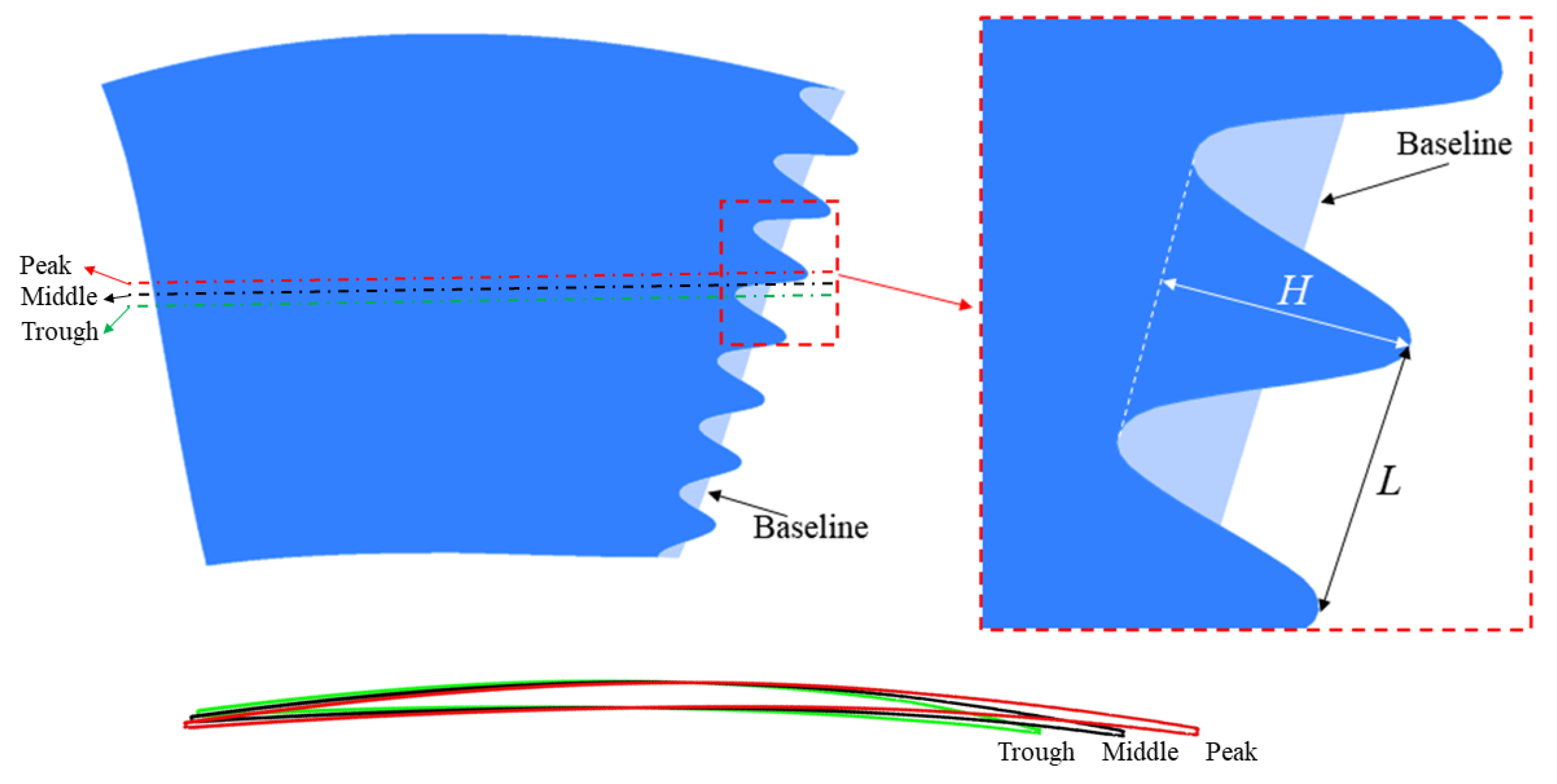
Figure 3.
Computational domain.

Figure 4.
Computational mesh on baseline fan.
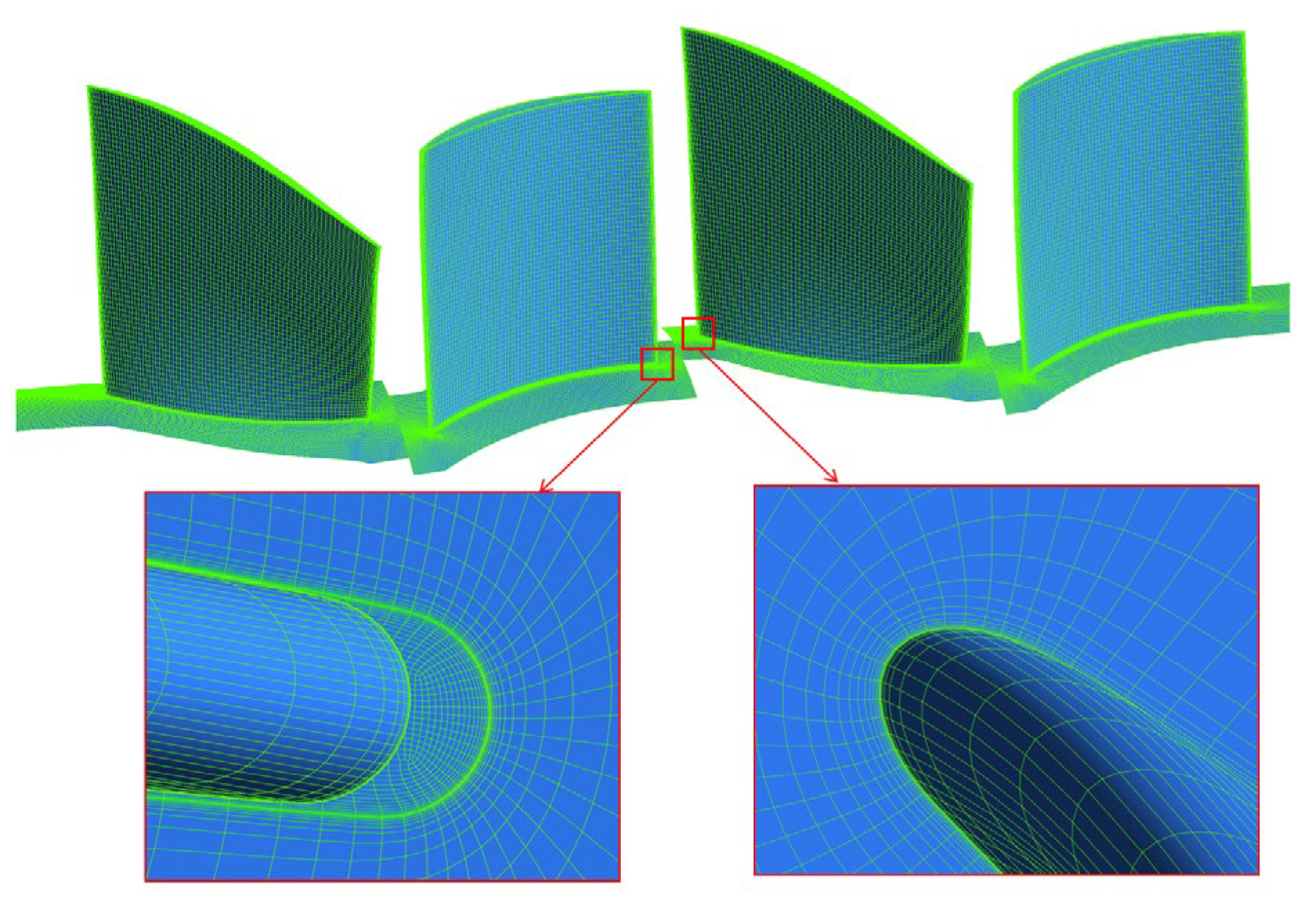
Figure 5.
The y+ distribution of blades and vanes. (a) Suction surface; (b) pressure surface (based on S1).
Figure 5.
The y+ distribution of blades and vanes. (a) Suction surface; (b) pressure surface (based on S1).

Figure 6.
Fan vane blade ‘strip’ processing and acoustic calculation diagram: (a) Stator vanes ‘stripped’; (b) Load solving; (c) Noise solution.
Figure 6.
Fan vane blade ‘strip’ processing and acoustic calculation diagram: (a) Stator vanes ‘stripped’; (b) Load solving; (c) Noise solution.

Figure 7.
Comparison of TKE and TLS for baseline fan with different meshes: (a) circumferential average TKE along span in front of S1; (b) circumferential average TLS along span in front of S1; (c) circumferential average TKE along span in front of S2; (d) circumferential average TLS along span in front of S2.

Figure 8.
Comparison of experimental result and predicted results for cascade [31]: (a) Grid 1; (b) Grid 2.
Figure 8.
Comparison of experimental result and predicted results for cascade [31]: (a) Grid 1; (b) Grid 2.
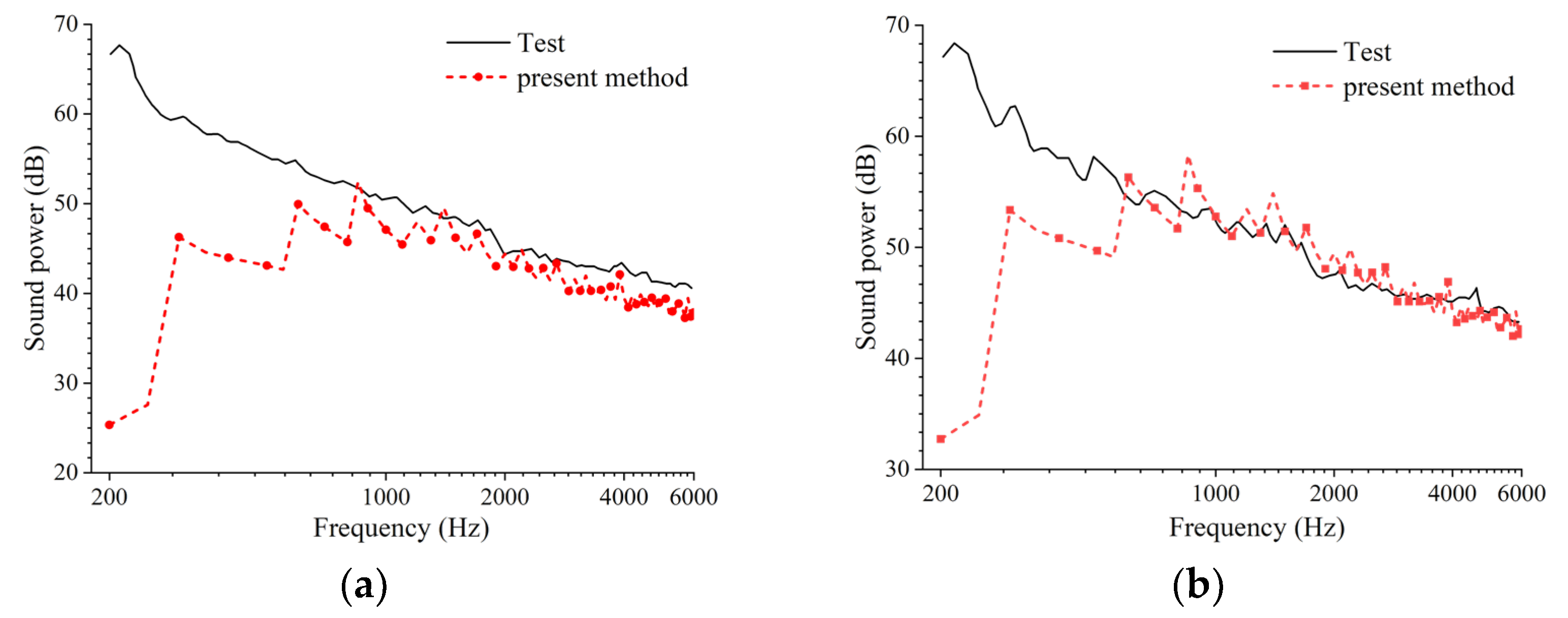
Figure 9.
PWL of R1–S1 interaction noise with change in wavelength: (a) H/L = 1; (b) H/L = 1.5; (c) H/L = 2.
Figure 9.
PWL of R1–S1 interaction noise with change in wavelength: (a) H/L = 1; (b) H/L = 1.5; (c) H/L = 2.

Figure 10.
PWL of R1–S1 interaction noise on baseline fan and H20L10 bionic fan.

Figure 11.
PWL of R1–S1 interaction noise with change in H/L: (a) L = 6; (b) L = 8; (c) L = 10.

Figure 12.
PWL of S1–R2 interaction noise on baseline fan and bionic fans.

Figure 13.
PWL of R2–S2 interaction noise on baseline fan and bionic fans.

Figure 14.
Circumferential averaged TKE along span for the baseline and bionic blades: (a) H/L = 2; (b) L = 10.
Figure 14.
Circumferential averaged TKE along span for the baseline and bionic blades: (a) H/L = 2; (b) L = 10.

Figure 15.
Circumferential averaged TLS along span for the baseline and bionic blades: (a) H/L = 2; (b) L = 10.
Figure 15.
Circumferential averaged TLS along span for the baseline and bionic blades: (a) H/L = 2; (b) L = 10.
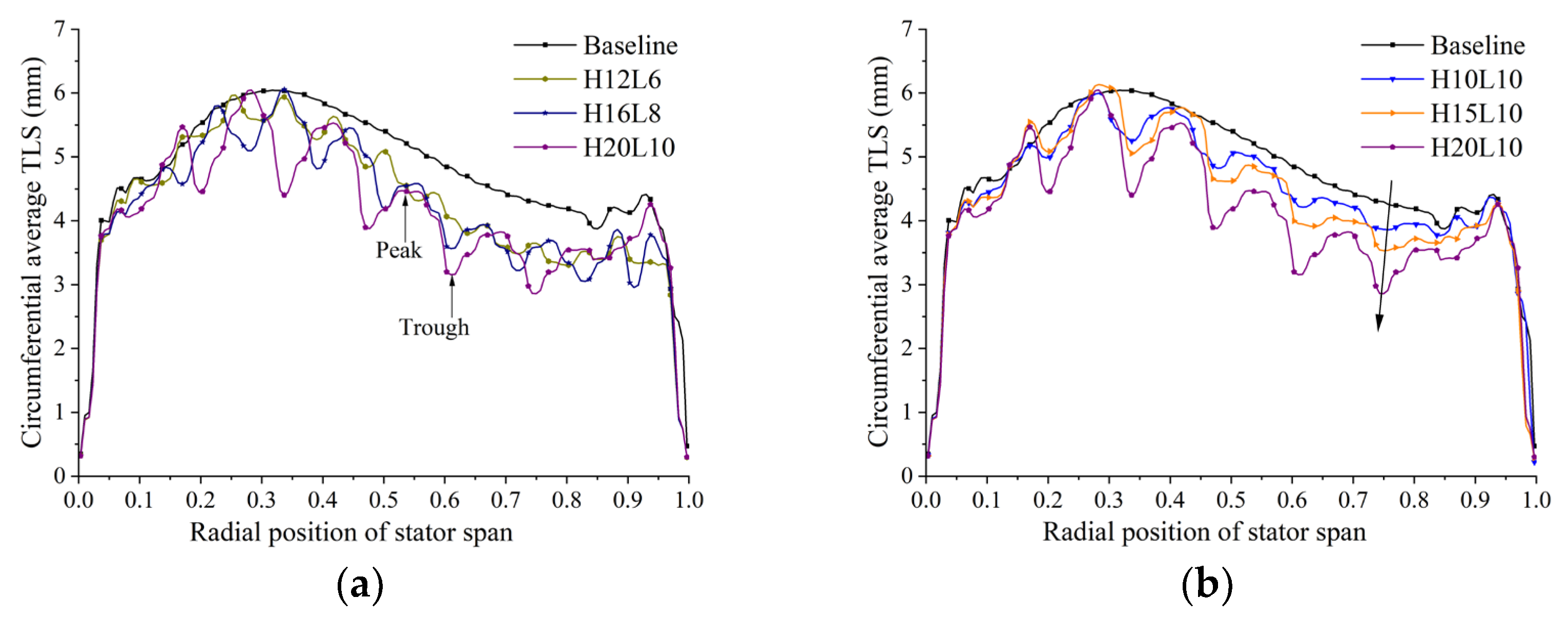
Figure 16.
TKE distribution in the wake region of R1 for the baseline and bionic blades: (a) Baseline; (b) H10L10; (c) H15L10; (d) H20L10.
Figure 16.
TKE distribution in the wake region of R1 for the baseline and bionic blades: (a) Baseline; (b) H10L10; (c) H15L10; (d) H20L10.

Figure 17.
Effect of wavy trailing-edge on wake at the 60% span.

Figure 18.
Vorticity distribution of R1 for the baseline and bionic blades: (a) Baseline; (b) H20L10.
Figure 18.
Vorticity distribution of R1 for the baseline and bionic blades: (a) Baseline; (b) H20L10.


Table 1.
Key parameters of two-stage fan.
| Parameters | Data |
|---|---|
| R1 blades | 18 |
| S1 vanes | 20 |
| R2 blades | 22 |
| S2 vanes | 24 |
| Shroud diameter (mm) | 500 |
| Hub diameter (mm) | 300 |
| Tip clearance (mm) | 1 |
| Design speed (rpm) | 5000 |
| Design mass flow (kg/s) | 8.5 |
| Total pressure ratio | 1.1 |
Table 2.
Design parameters of wavy trailing-edge blades.
| Model | L | H/L | H |
|---|---|---|---|
| H6L6 | 0.06c | 1 | 0.06c |
| H9L6 | 0.06c | 1.5 | 0.09c |
| H12L6 | 0.06c | 2 | 0.12c |
| H8L8 | 0.08c | 1 | 0.08c |
| H12L8 | 0.08c | 1.5 | 0.12c |
| H16L8 | 0.08c | 2 | 0.20c |
| H10L10 | 0.10c | 1 | 0.10c |
| H15L10 | 0.10c | 1.5 | 0.15c |
| H20L10 | 0.10c | 2 | 0.20c |
Table 3.
Mesh independence study for baseline fan.
| Baseline | Elements Number () | |||
|---|---|---|---|---|
| Mesh1 | Mesh2 | Mesh3 | Mesh4 | |
| R1 | 0.65 | 0.88 | 1.35 | 2.31 |
| S1 | 0.69 | 0.94 | 1.33 | 1.94 |
| R2 | 0.52 | 0.70 | 1.01 | 1.53 |
| S2 | 0.87 | 1.36 | 1.74 | 2.70 |
| Total | 2.73 | 3.88 | 5.43 | 8.48 |
| γ | 1.1013 | 1.1014 | 1.1015 | 1.1015 |
| η | 89.1018 | 89.1530 | 89.1535 | 89.1547 |
Table 4.
Mesh independence study for wavy trailing-edge blades.
| Model | η (%) | ηerror (%) | Model | η (%) | ηerror (%) | Model | η (%) | ηerror (%) | |||
|---|---|---|---|---|---|---|---|---|---|---|---|
| H6L6 | 1.53 | 89.1677 | 0.0082 | H8L8 | 1.69 | 89.1378 | 0.0465 | H10L10 | 1.69 | 89.1249 | 0.0132 |
| 2.01 | 89.1604 | --- | 2.11 | 89.1793 | --- | 2.06 | 89.1367 | --- | |||
| 2.54 | 89.1615 | 0.0012 | 2.67 | 89.7827 | 0.0038 | 2.61 | 89.1388 | 0.0024 | |||
| H9L6 | 1.73 | 89.1610 | 0.0324 | H12L8 | 1.70 | 89.1496 | 0.0430 | H15L10 | 1.78 | 89.1420 | 0.0037 |
| 2.06 | 89.1312 | --- | 2.03 | 89.1113 | --- | 2.14 | 89.1453 | --- | |||
| 2.34 | 89.1228 | 0.0094 | 2.34 | 89.1168 | 0.0062 | 2.55 | 89.1440 | 0.0015 | |||
| H12L6 | 1.51 | 89.1127 | 0.0092 | H16L8 | 1.49 | 89.1064 | 0.0726 | H20L10 | 1.48 | 89.0837 | 0.0149 |
| 2.05 | 89.1045 | --- | 2.11 | 89.1711 | --- | 2.05 | 89.0970 | --- | |||
| 2.61 | 89.1092 | 0.0053 | 2.70 | 89.2111 | 0.0449 | 2.49 | 89.0916 | 0.0061 |
Table 5.
Total pressure ratio and isentropic efficiency of bionic fan.
| Model | L | H/L | (%) | (%) | ||
|---|---|---|---|---|---|---|
| Baseline | --- | --- | 1.1015 | --- | 89.15 | --- |
| H6L6 | 0.06c | 1 | 1.1012 | −0.03 | 89.16 | 0.01 |
| H9L6 | 0.06c | 1.5 | 1.1008 | −0.06 | 89.13 | −0.02 |
| H12L6 | 0.06c | 2 | 1.1002 | −0.12 | 89.11 | −0.04 |
| H8L8 | 0.08c | 1 | 1.1011 | −0.04 | 89.18 | 0.03 |
| H12L8 | 0.08c | 1.5 | 1.1005 | −0.09 | 89.11 | −0.04 |
| H16L8 | 0.08c | 2 | 1.0999 | −0.15 | 89.17 | 0.02 |
| H10L10 | 0.10c | 1 | 1.1009 | −0.05 | 89.14 | −0.01 |
| H15L10 | 0.10c | 1.5 | 1.1002 | −0.12 | 89.14 | −0.01 |
| H20L10 | 0.10c | 2 | 1.0994 | −0.19 | 89.10 | −0.06 |
Disclaimer/Publisher’s Note: The statements, opinions and data contained in all publications are solely those of the individual author(s) and contributor(s) and not of MDPI and/or the editor(s). MDPI and/or the editor(s) disclaim responsibility for any injury to people or property resulting from any ideas, methods, instructions or products referred to in the content. |
© 2024 by the authors. Licensee MDPI, Basel, Switzerland. This article is an open access article distributed under the terms and conditions of the Creative Commons Attribution (CC BY) license (https://creativecommons.org/licenses/by/4.0/).
Share and Cite
MDPI and ACS Style
Gao, R.; Chen, W.; Tong, H.; Lian, J.; Qiao, W. Broadband Noise Reduction of a Two-Stage Fan with Wavy Trailing-Edge Blades. Aerospace 2024, 11, 374. https://doi.org/10.3390/aerospace11050374
AMA Style
Gao R, Chen W, Tong H, Lian J, Qiao W. Broadband Noise Reduction of a Two-Stage Fan with Wavy Trailing-Edge Blades. Aerospace. 2024; 11(5):374. https://doi.org/10.3390/aerospace11050374
Chicago/Turabian StyleGao, Ruibiao, Weijie Chen, Hang Tong, Jianxin Lian, and Weiyang Qiao. 2024. "Broadband Noise Reduction of a Two-Stage Fan with Wavy Trailing-Edge Blades" Aerospace 11, no. 5: 374. https://doi.org/10.3390/aerospace11050374
Note that from the first issue of 2016, this journal uses article numbers instead of page numbers. See further details here.