
An Ad Hoc Procedure for Testing Serial Correlation in Spatial Fixed-Effects Panels

Dipartimento di Scienze Economiche, Aziendali, Matematiche e Statistiche (DEAMS), University of Trieste, 34127 Trieste, Italy
Mathematics 2024, 12(10), 1475; https://doi.org/10.3390/math12101475
Submission received: 27 March 2024
/
Revised: 24 April 2024
/
Accepted: 4 May 2024
/
Published: 9 May 2024
(This article belongs to the Special Issue Mathematical Economics and Spatial Econometrics)
Abstract
:We consider testing for error persistence in spatial panels with (potentially correlated) individual heterogeneity. We propose two variants of an ad hoc testing procedure based on first transforming out the individual effects, either by time-demeaning or by taking forward orthogonal deviations, then estimating an encompassing spatio-temporal model. The procedure can also be employed under the random effects assumption, in which case, although suboptimal, it can be computationally cheaper and safer than existing tests. We report Monte Carlo simulations demonstrating satisfactory empirical properties.
1. Introduction
It is uncommon for empirical spatial panel analysts to test for serial error correlation, not least because of a lack of infrastructure. In fact, while there has been substantial attention in the methodological literature to the uncorrelated heterogeneity/“random effects” case (see in particular [1]), there are no readily available tests for serial error correlation in the important case when the individual heterogeneity is allowed to be correlated with the explanatory variables (so-called “fixed effects”). This is in contrast with the more popular spatial dependence tests, where many recent contributions have been devoted to the fixed effects case [2,3,4,5], and also further specification issues like Hausman testing [6] or general error “sphericity” [7].
Time is usually incorporated in standard spatial panel models under the form of time dummies, which account for non-space-related correlation in the cross-section, and of individual, time-invariant effects, which account for the persistence in time of individual-specific characteristics. On the converse, time-decaying serial error correlation of the kind exemplified, in the simpler case, by a first-order autoregressive process is rarely considered in this field. This is unfortunate because the efficiency of maximum likelihood estimation hinges on an i.i.d. assumption for the remainder errors, which would be violated by the presence of serial correlation (for a comparison of estimates of static spatial models with or without serial error correlation, see [8], Tables 4 to 6).
Dynamic spatial panel models, where the dependent variable follows an autoregressive process, are an active research area (see e.g., [9,10,11,12]) with plenty of empirical applications. In applied work on static panels, on the other hand, all attention does usually go to spatial correlation features, and serial dependence in the errors is seldom tested [13], despite the fact that, as per Griffith [14], “time rather than geographic dependency dominates the structuring of information in space-time data cubes”: i.e., correlation in time is generally likely to be stronger than in space.
There are important differences in both economic interpretation and estimation between dynamic models and static ones with autocorrelated errors. As often happens, though, these are less pronounced on the testing side: maintaining the null of uncorrelated errors in a static model on stationary data—the appropriate condition for meaningful estimation of a static spatial panel model through the usual Maximum Likelihood (ML) or Generalized Moments (GM) methods—either feature will cause a serial correlation-testing statistic to diverge. In other words, whether one approaches the issue of time persistence under the form of serial error correlation, or rather based on the specification of a dynamic model (see e.g., [15]), testing for serial error correlation as a diagnostic check is nevertheless relevant in both approaches, as any omitted dynamics would show up in error persistence. Moreover, very strong serial correlation, emerging either in the form of an estimated parameter near 1 (see the example in Section 5) or of extremely high test statistics, can signal a nonstationarity problem, suggesting the need to reconsider the specification in a broader sense.
This paper sets out to address the issue of testing for serial error correlation proper (i.e., of the time-decaying type) in spatial panels while accounting for individual effects of the fixed type, which are the most general specification and encompass the case of random-type effects. In doing so, we aim to provide practical guidance to researchers who want to check their specification against the above features. If any standard spatial panel (static, with either a spatial lag, a spatial error, or both, and with individual effects) does not “pass” the residual serial correlation test, then it is due for thorough respecification because the consequences are most likely to be serious. In fact, either of the three misspecifications (omission of a lagged dependent variable; omission of serial correlation in the error term; and error nonstationarity) will cause inconsistency of the standard ML estimator.
In particular, we suggest two feasible testing strategies based on eliminating individual effects altogether—i.e., generally applicable without making any assumption on the nature of individual fixed effects and their correlation with the regressors. The first is based on time-demeaning and inspired by Wooldridge [16]; the second is based on taking forward orthogonal deviations of the data in the spirit of Lee and Yu [17] and Debarsy and Ertur [2]. In both cases, the full spatial model (including serial error correlation) is estimated using transformed data, then the resulting serial correlation coefficient is tested for departures from the appropriate derived null hypothesis—which depends on the transformation employed—corresponding to the original null of no serial error correlation.
In the following, after a brief review of the literature, we set out the general model with unobserved heterogeneity, spatial lags and both spatially and serially correlated errors; then we review ML estimation thereof and describe the transformation needed to eliminate the fixed effects. In Section 3, we outline the testing procedure. Section 4 contains a motivating example, exposing serial correlation in a well known model from the spatial panel literature. Section 5) is dedicated to a Monte Carlo assessment of the properties of the proposed tests in finite samples, with special attention to the small sizes frequently appearing in applied literature. Conclusions follow.
1.1. Literature Review and Background
Testing for serial correlation has often been overlooked so far in the spatial panel literature, with a few notable exceptions. Baltagi et al. [1] have extended the spatial panel framework to serial correlation in the remainder errors, deriving joint and conditional tests (see in particular their C.2 statistic), while Elhorst [18] has considered simultaneous error dependence in space and time. Lee and Yu [13] proposed a very general specification including spatial lags, spatially and serially correlated errors together with individual effects. They assess the biases due to neglecting serial correlation or some part of the spatial structure through Monte Carlo simulation, and recommend a general to specific model selection strategy. Yet this line of research has seen more methodological contributions (see also [19]) than empirical applications. For example, we surveyed all the 481 Google Scholar citations of the seminal paper Baltagi et al. [1] at the end of 2023, discovering that most are either in methodological papers, or—the majority—in applied papers taking inspiration from their general framework but not really employing the proposed serial correlation test. In fact, the only studies actually performing a C.2 serial correlation test in a spatial context are Bouayad-Agha et al. [20], Millo and Carmeci [21], Millo and Carmeci [22], Aravindakshan et al. [23], Lottmann [24], Kunimitsu et al. [25], Lim-Wavde et al. [26], Olivier and Del Lo [27] and Sadewo et al. [28]: all this when a user-friendly R implementation of the C.2 has long been available (see [29], Section 10.4.2.1). As Lee and Yu observe, “[i]n empirical applications with spatial panel data, it seems that investigators tend to limit their focus on some spatial structures and ignore others, and in addition, no serial correlation is considered” [13] (p. 1370).
The literature has until now concentrated on the random effects (RE) case. For testing serial correlation in spatial pooled or RE panels (tests devised under the RE hypothesis will in general be consistent under the special case of the pooled model), all three classic likelihood-based testing procedures are available. In a Lagrange Multipliers (LM) framework, one can use the C.2 test of Baltagi et al. [1] if the model has spatially correlated errors (but no spatial lag). In a spatial lag panel setting, with or without RE, one can instead follow Montes-Rojas [19]. The comprehensive estimation framework for static panels described in Millo [8] allows estimating either the general, encompassing model with both spatial (-lag as well as -error) and serial correlation, or the restricted case without serial correlation. Likelihood ratio (LR) tests of the restriction of no serial correlation are therefore possible, while allowing for spatial and/or random effects. Analogously, from within the encompassing model, the significance diagnostics for the autoregressive parameter amount to a Wald test for serial correlation, asymptotically equivalent to the LR test mentioned above.
The above techniques cannot be directly applied to fixed effects (FE) panels, which on grounds of robustness are often the preferred alternative in many applied fields, as macroeconomics, regional applications, or political science (in fact, as the argument goes, sets of countries or regions cannot be seen as having been drawn randomly from a population, but rather as being the population itself: see Elhorst [10] (Chapter ii); in favour of the random effects view, see Mátyás and Sevestre [30] (Introduction)). This paper regards the proposal of a feasible strategy for testing serial error correlation in static spatial panels of a rather general nature. Devised for the fixed effects case, the testing procedure is not limited to one of the spatial lag and spatial error types but allows for either one, and possibly for combinations of the two. It encompasses the cases of random or no individual effects, given that the individual effects—if any—are eliminated altogether by transformation.
It must be stressed that no formal results are presented regarding the consistency of the proposed tests, which build upon existing estimation procedures. Yet the simulation results presented below suggest that they can be very useful in signalling a serial correlation problem, acting as a stopgap for empiricists until a desirable optimal test for serial correlation under spatial and fixed effects is derived.
2. The Model
Our point of departure is the spatial panel data regression model with serially and spatially correlated errors described in Millo [8] (The model in Millo [8] is, as discussed there, itself both an extension of that of Baltagi et al. [1]—which did not include a spatial lag—and a particularization of that in Lee and Yu [17]—which adds moving average terms).
where is the vector of observations on each cross-sectional unit i in each time period t, with and , stacked by cross-section (so that time is the slowest index), and X is a matrix of observations on the k regressors (which may contain time dummies). As usual, W indicates the matrix of known spatial weights whose diagonal elements are set to zero, and is the identity matrix of order T. Moreover, is assumed to be non-singular.
The disturbance vector is the sum of individual effects and spatially autocorrelated errors. In vector form, for each cross-section, this can be written as
The spatial correlation in the errors is supposed, for simplicity, to share the same spatial structure as the dependent variable, described in the proximity matrix W. This assumption can be easily relaxed employing two separate spatial matrices , .
The remaining disturbance term follows a first-order serially autocorrelated process. Again, for each cross-section,
, , and are all columns vectors, is the random vector of region specific effects; () is the spatial autoregressive coefficient and () is the serial autocorrelation coefficient. Finally, and are assumed to be iid Normal, and independent of each other. is assumed to be non-singular. No assumptions are made, consistently with the FE approach, on the correlation between the individual effects and the regressors X; while the latter are assumed exogenous with respect to the idiosyncratic errors e. In the following, nevertheless, we will refer to the random effects (RE) hypothesis—the assumption of independence between and X—as a special case of our setting.
The model allows for serial correlation on each spatial unit over time as well as spatial dependence between spatial units at each time period. The presence of individual effects accounts for possible heterogeneity across spatial units.
Eliminating Fes by Transformation
If the exogeneity assumption for individual effects (RE hypothesis) did hold, individual effects could be kept as part of a spatio-temporal model. Random effects models with spatial and serial correlation can in fact be estimated by maximum likelihood; Millo [8] (Section 4) describes the iterative procedure. Statistical inference can then be based on the information matrix. Millo [8], Millo and Piras [31] obtain standard errors for from GLS, and employ a numerical Hessian to perform statistical inference on the error components. These steps remain valid for particular restrictions of the general model: the specification without individual effects () will be of interest in our case.
In the more general case where the RE assumption does not hold, to avoid endogeneity concerns, the individual effects have to be either controlled for explicitly or, as is more often the case, eliminated before estimation. This elimination is usually accomplished by either differencing or time-demeaning the data (see [16], Section 10.5), or through the orthogonal deviations transformation popularized by Arellano and Bover [32]. Once the fixed effects have been transformed out, a restricted version of the above model assuming can be estimated.
The well-known time-demeaning, or within transformation entails subtracting averages over the time dimension, so that the model is estimated using the transformed data:
where and denote time means of and X. Standard FE models are estimated through OLS using time-demeaned data. According to the framework of Elhorst [33], fixed effects estimation of spatial panel models is also accomplished as pooled ML estimation using time-demeaned data. Elhorst’s procedure has long been the standard in applied practice, but has been questioned by Anselin et al. [34] because time-demeaning alters the properties of the joint distribution of errors, introducing serial dependence; although, as it turns out, the estimates of and spatial parameters remain consistent: see Lee and Yu [35] (p. 257) for a discussion of the issue, and Millo and Piras [31] (p. 33) for Monte Carlo evaluation of its practical significance. To solve the problem, Lee and Yu [17] (3.2) suggest to apply a different transformation which is well known from the panel data literature as forward orthogonal deviations (henceforth OD) and has been proposed by Arellano and Bover [32] (pp. 41–42) in the context of dynamic, non-spatial panels (see also [36], p. 17). The transformed data are then, for any variable (e.g., y),
for ; one time period is lost in the transformation. In the case of the model containing only individual effects, estimated by OLS on transformed data, the two data transformations are equivalent as regards estimating the parameter of interest : in fact, . From our viewpoint, the OD transformation has the desirable characteristic of preserving the correlation structure of the errors; i.e., differently from the FE transformation, of not inducing any artificial serial correlation in the transformed errors (for a formal illustration of this last point, see [2], Section 2).
3. Testing for Serial Correlation
In this section, we outline the testing procedure for assessing serial correlation in the remainder errors of the spatial model described by Equations (1)–(3). The null hypothesis is that in Equation (3). The test is based on the maximum likelihood estimate of the serial correlation coefficient in the model on transformed data:
where denotes a transformation of the data which (a) cancels out the individual heterogeneity, and (b) does possibly modify the original serial correlation parameter to . As it happens, the two transformations we consider here do also preserve the regression parameters of the original model, and, if any, the spatial ones but this is inessential to our purposes.
The testing procedure will take the form of a Wald-type linear restriction test on the parameter . The linear hypothesis under test will be derived from the original null .
We take inspiration from a general testing procedure for serial correlation in fixed effects panel models, described in Wooldridge [16] (Section 10.7.2) in the context of non-spatial panels. i.e., put in our setting, he considers testing for assuming that both in Equation (1) and in Equation (2) (Wooldridge [16] describes two different ways to test for serial correlation drawing on transformed residuals: one, based on taking first differences, has been popularized by Drukker et al. [37]; we concentrate on the other, less popular proposal, based on time-demeaning the data, because it is more appropriate for stationary data than the differencing way). In the latter case (non-spatial, pooled model without individual effects), under the null of no serial correlation in the idiosyncratic errors, the regression residuals of the pooled model must be uncorrelated. The same is true if individual effects have been eliminated by OD, which preserves the original properties of the idiosyncratic errors—but eliminates information for one time period. In the FE case, on the other hand, if the original model’s errors are uncorrelated then we expect the residuals from the quasi-demeaned regression to be negatively serially correlated, with for each t (see [16], Section 10.5.4). This correlation disappears as T diverges, so standard serial correlation tests can be readily applied to panel data with large T (see [38], Section 2.3 and Formula 12).
By analogy, the idea of transforming out the individual effects and then evaluating a derived null hypothesis can be extended to other settings, provided that one can draw on a consistent estimator for . In the case of our interest, testing for serial correlation in the errors of spatial panels can be addressed this way provided that the spatial features of the model are appropriately taken into account. This can be carried out in the comprehensive estimation approach including serial correlation mentioned above: i.e., transforming the data through either FE or OD, then estimating the original model on transformed data, omitting the individual effects which have now been transformed out, and assessing . For any , the likelihood of a model with spatial and serial correlation but no individual effects is reported in Millo [8] (pp. 922–923), where estimation is also discussed.
Two different tests can be performed on the estimates, depending on the way individual effects have been transformed out, as the transformation employed determines the derived null hypothesis. If using OD, the derived null hypothesis resembles the original: . Let us denote the Wald restriction test for based on ML estimation of the model (6) on data in orthogonal deviations:
Given that the estimated model is well-specified under the null, this statistic can be expected to tend, asymptotically, to .
In the FE transformation case, if the original model’s errors are uncorrelated, then FE residuals are negatively serially correlated, with for each t (see [16], Section 10.5.4). This correlation disappears only as T diverges; for any finite T, the derived null hypothesis becomes . We call the Wooldridge-type AR(1) test for spatial panels based on testing based on ML estimation of the model (6) on time-demeaned data:
Again, the estimated model is well-specified under the null (in particular, it allows for serial error correlation), so this statistic can in turn be compared with .
Rejecting either of the above restrictions would make us conclude against the original null of no serial correlation in the original model. Notice that the ML model in Equation (6), leaving free to vary, is well specified under for both alternative procedures.
It shall be observed that testing procedures appropriate under the FE assumption are a fortiori so under the more restrictive random effects (RE) assumption, whereby the individual effects are uncorrelated with the regressors. Although under RE the encompassing model can be directly estimated without need for transforming the data, the demeaning-based approach is still valid. The above likelihood turns out to be much easier to optimize with respect to the one including random individual effects, on which optimal Wald or likelihood ratio tests can be based (on the computational issues in general, see [8], Section 5). Moreover, ML estimation of the model without random effects, although including serial correlation, still turns out computationally simpler than that of the spatial random effects model, whose residuals are needed as the basis for the conditional LM test (C.2) of Baltagi et al. [1] (see [8], Table 2, (sar+)semsr vs. (sar+)semre). Hence, employing a FE-type test based on elimination of the individual heterogeneity, although suboptimal under RE, can turn out to be both a more robust and a computationally less burdensome alternative under the RE hypothesis as well—besides being the only viable choice under FE.
One last observation is that, being based on ML estimation of the transformed model, both testing procedures depend on an assumption of normality of the remainder errors. In the same line of reasoning, but more in general, they also depend on the space-time dependence being correctly modelled by Equations (1)–(3); in principle, alternative data generating processes (like e.g., that of [18]) would require the likelihood to be respecified: although it can be conjectured that the tests maintain power towards misspecified alternatives, this would require a formal proof. The results from robustness checks (reported in Appendix A) are nevertheless encouraging.
4. Monte Carlo Experiments
To assess the performance of and in real-world conditions through Monte Carlo simulation, we consider the rejection rates of either test at the 5% significance level: this corresponds to the empirical size if the data are simulated under the null hypothesis of no serial correlation, and to the empirical power of the test under alternative data generating processes where .
The simulation design is a generalization of that in Millo and Piras [31] (Section 8). The idiosyncratic innovations are distributed as a standard Normal, and the individual effects as , so that is also the ratio of error variances. Along with an intercept term, we consider two regressors: is sampled from a Uniform [−7.5, 7.5], is drawn from a standard Normal. The simulation parameters are chosen with a target of . The coefficients for the regressors are set to and 10, respectively. Our spatial layout is given by the 48 states of the continental US. The spatial weighting matrix is a simple binary contiguity one. We consider three values for the number of time periods, the lowest representative of a typical “short” panel, the highest of macroeconomic panels found in the literature, and set . We allow combinations of two different values for both and , namely either zero (no effect) and , so that next to the usual two cases of spatial lag (SAR) and spatial error (SEM), we consider both the case of no spatial correlation and that of combined SAR and SEM processes. We consider three values for the objective parameter : zero, corresponding to no error persistence, and two positive levels of serial correlation: (weak) and (strong). For all experiments, 1000 replications are performed, so that the 95% confidence bands for the empirical size based on the binomial distribution are 0.036 and 0.064 (Table 1).
Test size under validity of the null is reasonably close to 5% in all experiments, more so when T = 10–15 than in the short panel. Empirical power is very good for the long panels both for weak () and for strong () error persistence; in the short panel case, power is moderate (near 50%) for the test, while lower for the variant. Results are much the same under either type of spatial dependence, both or none alike, and under presence or absence of individual effects, testifying how effectively the procedure controls for spatial and idiosyncratic features. The test uniformly dominates the over the short sample; for the longer panel, the results of the former are still slightly better, but in this case performance is satisfactory for both versions so that either can be safely employed (Table 2).
The proposed procedures prove effective in testing for serial error correlation in spatial panels of lag and/or error type containing correlated individual heterogeneity. Because elimination of the individual effects through transformation is appropriate—although statistically suboptimal—under the random effects hypothesis as well, these FE-type tests can be safely employed in dubious situations as regards the exogeneity of the effects. Being computationally both cheaper and more robust than their RE counterparts, they can also be employed in numerically problematic situations.
5. Illustrations
To illustrate the use (and the relevance) of the different tests, we will resort to some well-known examples of spatial panels: one (Italian insurance) with a strong degree of serial error correlation, but still no evidence of nonstationarity; another (Indonesian rice farming) with mild serial correlation; and the last (the well-known Cigarette dataset) where a static specification is outright inappropriate, in order to illustrate how investigating serial correlation can reveal nonstationarity issues.
We consider random effects settings, allowing us to compare and to established tests and procedures: the joint test of Baltagi et al. [1]; the conditional serial correlation test of Baltagi et al. [1]; and the Likelihood Ratio and Wald tests equivalent to , from estimating the encompassing model, and the estimated coefficient from the latter.
It must be borne in mind, though, that—unlike the rest— and would be appropriate in a fixed effects setting as well. In turn, and are feasible in a (random effects) SAR + SEM setting, while and only allow for SEM.
5.1. Italian Insurance
The Italian insurance example from Millo and Carmeci [21], as mentioned in Section 1.1, was among the first empirical applications of the Baltagi et al. [1] C.2 conditional LM test. Per-capita insurance expenditure in 103 Italian provinces is regressed on a set of drivers (income, wealth, population density, cost of borrowing, agencies’ network density, education, share of agriculture, average family size), some of which have limited (or no) time variation, which makes a fixed effects regression infeasible. The model therefore takes into account a mix of correlated and uncorrelated heterogeneity at different geographical levels: fixed macroregional effects and unit (i.e., provincial) random effects. Spatial correlation is introduced through a SEM term. It then becomes possible to employ the C.2 test for spatial error correlation, allowing for both serial correlation and random effects. The same example is extended to a SAR + SEM setting in Millo [8] (Section 6.2), where a more complex spatial structure emerges from the data. In both cases, there is evidence of serial error correlation.
In Table 3, all tests mentioned in the paper are performed first on the spatial error specification (upper panel). The available procedures are then applied to the more general SAR + SEM specification (lower panel). LM tests are not reported, being inappropriate in this latter case, as they have been derived for a SEM model.
Under the random effects hypothesis, the upper left part of the table can be considered: , and Wald-type tests and the estimate of . All likelihood-based tests signal a very strong departure from the null of serial uncorrelation, while from estimation of the comprehensive model is “large” but far from one: consistent with stationarity. The and tests also reject the null well beyond any conventional significance level.
If the random effects hypothesis were considered dubious, then one could only look at the results from the and tests; again, there is little doubt about serial correlation in the error terms of the present example.
5.2. Indonesian Rice Farming
The rice farming example [39] draws on 171 rice farms located in six different villages of the Chimanuk River basin in West Java (Indonesia), observed over six growing seasons, three wet and three dry, between 1975 and 1983. A production frontier equation is estimated, relating rice output to the following inputs: seed, urea, phosphate, labour hours and land (size), all but phosphate in logs (Dummy variables accounting for the use of high yield varieties of seed, or for a mix of seed varieties and for the use of pesticides, and for the six villages and for the season being a wet one are included in the original specification but omitted here for the sake of simplicity). Following Druska and Horrace [39], the proximity matrix is constructed considering all the farms of the same village as neighbours.
Spatial correlation between farms belonging to the same village can be expected; a spatial error process seems theoretically more appropriate, due to spillovers across neighbouring farms in climate and generic local factors affecting production, while it is less easy to justify the inclusion of a spatial lag of the dependent variable: in fact, estimating the encompassing SAR + SEM model yields strong SEM dependence but no evidence of SAR (see [8], Section 6.1). In the following, for the sake of illustration, we will nevertheless consider this last case as well.
Again, in Table 4, all tests mentioned in the paper are performed on a static spatial error specification, then those appropriate are applied to the more general SAR + SEM specification.
Under the random effects hypothesis, in the left part of the table all likelihood-based tests signal a mild departure from the null of serial uncorrelation, from estimation of the comprehensive model being modestly sized. The and tests also reject the null: just so, in line with the other procedures, more strongly.
5.3. Cigarettes
The Cigarette dataset is taken from Baltagi [40] (the spatial weights matrix is due to Paul Elhorst; data and weights can be found, respectively, in the R packages Ecdat [41] and splm [31]). The original application is in Baltagi and Levin [42]. Further reconsiderations include Baltagi et al. [43], Baltagi and Griffin [44]. It contains data for the years 1963–1992 and 46 American states on the following: real per capita sales of cigarettes per person of smoking age (i.e., over 14) measured in packs, average real retail price per pack, real disposable income per capita and the minimum price per pack in neighbouring states. The last variable is included in the original application in order to proxy for cross-border smuggling [40] (p. 156); this could also be achieved controlling for spatial effects, as in the above-mentioned cases.
Individual (state-specific) effects are included to account for idiosyncratic characteristics of territory, like the presence of tax-exempt military bases or Indian reservations, the prevalence of a religion that forbids smoking (like in Utah) or the effect of tourism. Time effects are also included to account for (USA-wide) policy interventions and warning campaigns. Given their peculiar nature, both kinds of effects will better be assumed fixed; however, in the following we consider both testing under the RE and under the FE hypothesis.
The original application is dynamic, as it contains lagged consumption in order to control for habit persistence in smoking. Nevertheless, a static version of the Cigarette model has often been employed, mainly for illustration purposes, in a number of spatial econometric studies [45,46,47,48,49,50] and will therefore be familiar to most researchers. This latter we will use in our case, for the sake of illustration; given the theoretical reasons for persistence, it will be of particular importance to test for serial error correlation.
In the upper panel of Table 5, all tests mentioned in the paper are performed on the static spatial error specification. In the lower panel, the available procedures are applied to the more general SAR + SEM specification, again excluding LM tests as they have been derived for a SEM model.
If the random effects hypothesis can be trusted, the left part of the table can be considered: , and Wald-type tests and the estimate of . All likelihood-based tests signal a very strong departure from the null of serial uncorrelation, while from estimation of the comprehensive model is very near to one. The and tests also reject the null well beyond any conventional significance level. If the random effects hypothesis is considered dubious, then one can only look at the results from the and tests; again, there is little doubt about high persistence in the error terms. In any case, the results point to very strong autoregressive behaviour in the residuals, bordering with unit roots if we believe the RE hypothesis (under which is consistently estimated): a static spatial panel specification assuming timewise-uncorrelated errors is inappropriate, and an analysis of stationarity would be advisable.
Lastly, computing times for the and tests—based on production-quality implementations in R [51]—are smaller than those for their , and Wald counterparts by an order of magnitude; although all of them are still feasible on any machine for this, rather moderate, sample size. Not least, in larger samples they are less prone to errors due to numerical singularities in underlying procedures (see [8], Section 5.1.5 and Table 2, comparing either (sar+)semsrre estimators (needed for and ) or (sar+)semre () with (sar+)semsr ()).
6. Discussion, Limitations and Directions for Future Research
We address testing for serial error correlation in spatial panels of lag and/or error type, containing correlated individual heterogeneity. Comprehensive estimators both for the encompassing model and for its restrictions have been developed in the literature for the random effects case, as well as joint and conditional Lagrange multiplier tests (see references above), so that the zero-restriction of the serial correlation coefficient can be tested by either of the three well-known likelihood-based procedures. In contrast to the wealth of techniques available for the random effects case, the fixed effects case—which is often considered the most interesting one in spatial applications and is also appropriate (but for a loss of efficiency) in case the random effect assumption should hold true—has been given little attention.
We propose two feasible procedures for the fixed effects case, one based on observations in Wooldridge [16] and the other on the work of Lee and Yu [17] and Debarsy and Ertur [2]. The former consists in estimating the full spatial model on time-demeaned data and testing the resulting serial correlation coefficient for departures from the implied negative serial correlation induced by the demeaning transformation: the latter in employing, instead of time-demeaning, the forward orthogonal deviations transformation of Arellano and Bover [32]—which maintains the original correlation properties in transformed residuals but discards one time period—and directly testing the resulting coefficient for departures from zero.
Elimination of the individual effects through transformation is appropriate, although statistically suboptimal, even if the RE hypothesis holds; hence, our proposed FE-type tests, unlike the RE ones, can be safely employed in dubious situations. Moreover, the likelihood optimization procedure they are based upon is considerably simpler than that of the full model with RE, and has been proven to work even on relatively big samples. The computational burden from performing the proposed tests is actually smaller by an order of magnitude than that of the conditional C.2 test of Baltagi et al. [1], which requires the estimation of a spatial model with random effects.
A Monte Carlo experiment illustrates the size and power properties of the two proposed procedures, which turn out satisfactory for both tests when while the OD-based test fares better than the FE-based one in the short panel case (). We also empirically address, in further simulations (see the Appendix B), the robustness to partial misspecification of either the data generating process or the distribution of the errors. Again, the results are encouraging. The proposed procedures can be trusted to consistently signal a serial correlation problem in a wide range of applied situations. We provide them for empirical spatial econometrics researchers wanting to check for the presence of time persistence in their maintained model, in order to avoid the pitfalls mentioned in the Introduction, in a more structured and consistent way than simply looking at graphical depictions of the residuals (the latter being a useful first step nevertheless).
It must be noted, again, that we derive no formal results; based on intuitive arguments and established properties of the building blocks employed, we conjecture that they can be expected to be asymptotically distributed as a standard Normal. We do not simulate the entire distribution, concentrating instead on the quantile most relevant in empirical hypothesis testing (we thank an anonymous reviewer for insightful comments on this issue). We do not discuss higher-order serial correlation either; while from a testing viewpoint the proposed test will have power against an process (i.e., autocorrelation up to the p-th order), it might not detect autocorrelation at just a higher order, like, e.g., what can be expected at the fourth order in quarterly data.
The formal derivation of an optimal Lagrange Multiplier test for serial correlation like the C.2 of Baltagi et al. [1] for a fixed effects context is a desirable outcome of future research, as are tests for higher order serial correlation in spatial models. A related approach, which is also not pursued here, to assessing the presence of time-decaying persistence would be to estimate a dynamic model [9,17,52] and do a restriction test on the dynamic lag coefficient (we thank an anonymous reviewer for this observation).
Funding
This research received no external funding.
Data Availability Statement
Publicly available datasets were analyzed in this study. All are available within the R Project: the Italian Insurance dataset as “Insurance” in the package ‘splm’; the Rice Farming dataset as “RiceFarms” and the Cigarettes dataset as “Cigar”, both in package ‘plm’. The original sources are reported in the paper and in the online documentation.
Conflicts of Interest
The author declares no conflicts of interest.
Abbreviations
The following abbreviations are used in this manuscript:
| ML | maximum likelihood |
| GM | generalized moments |
| FE | fixed effects |
| RE | random effects |
| LM | Lagrange multiplier (test) |
| LR | likelihood ratio (test) |
| OLS | ordinary least squares |
| GLS | generalized least squares |
| OD | (forward) orthogonal deviations |
| SAR | spatially autoregressive (model) |
| SEM | spatial error model |
Appendix A. Robustness Checks
The procedure on which the tests are based relies on consistent ML estimation of the serial correlation coefficient. The latter depends on the correct specification of the model, both in terms of the data generating process with serial and spatial correlation, and in terms of the distribution of the idiosyncratic error terms. In the following, we address the consequences of (a) failing to specify the structure of the spatial-serial dependence or (b) assuming the wrong distribution for the error terms. From this perspective, the proposed tests will always be suboptimal under deviations from the ideal conditions of Normal remainder errors and perfectly specified data generating process. Given the practical orientation of the paper, and the fact that the ideal conditions will never really apply in real-world situations, here we are concerned with the effects of “far distant” misspecifications. Therefore we will consider, respectively, (a) a complete inversion of the order of spatial and serial dependence, and (b) grossly asymmetric viz. leptokurtic error distributions, quite unlikely to apply in practical situations.
Appendix A.1. Serial-Spatial Alternative Specification
To assess the robustness of the testing procedures to misspecification of the data generating process, we consider an alternative to the sequential way in which serial-spatial panel effects have been implemented since the seminal paper of Baltagi et al. [1], i.e., specifying the spatial processes as in Equations (1) and (2), then time-lagging the remainder error only, as in Equation (3). In this experiment we change the time-space dynamics of the error term, time-lagging the spatially correlated composite error:
In Table A1 we report empirical size and power for the tests in an experiment where the DGP is as in Equation (A1), for a combined SAR + SEM model with either or and no individual effects (). We choose and, as usual, . The results are practically indistinguishable from the corresponding ones for the “true” simulation DGP reported in Table 1 and Table 2.

Table A1.
Empirical size (bold) and power for the and tests for , for and T = 10, on the alternative DGP in Equation (A1). and are, respectively, the SEM and SAR spatial parameters. 2000 replications.
Table A1.
Empirical size (bold) and power for the and tests for , for and T = 10, on the alternative DGP in Equation (A1). and are, respectively, the SEM and SAR spatial parameters. 2000 replications.
| 0 | 0.058 | 0.050 | 0.059 | 0.053 |
| 0.1 | 0.397 | 0.360 | 0.407 | 0.381 |
| 0.2 | 0.929 | 0.920 | 0.927 | 0.919 |
| 0.3 | 0.999 | 0.999 | 1.000 | 0.999 |
| 0.4 | 1.000 | 1.000 | 1.000 | 1.000 |
Appendix A.2. Non-Normality
The ML estimator assumes normality of the remainder errors (e in Equation (6)). In order to assess the practical effects of misspecification in the error distribution, following Long and Ervin [53], we consider two alternative distributions to the Normal: one asymmetric (skewed to the left), the ; and one leptokurtic, with fatter tails than the Normal: the . Both are scaled to a standard deviation of one, while the is also centered on zero subtracting the expected value:
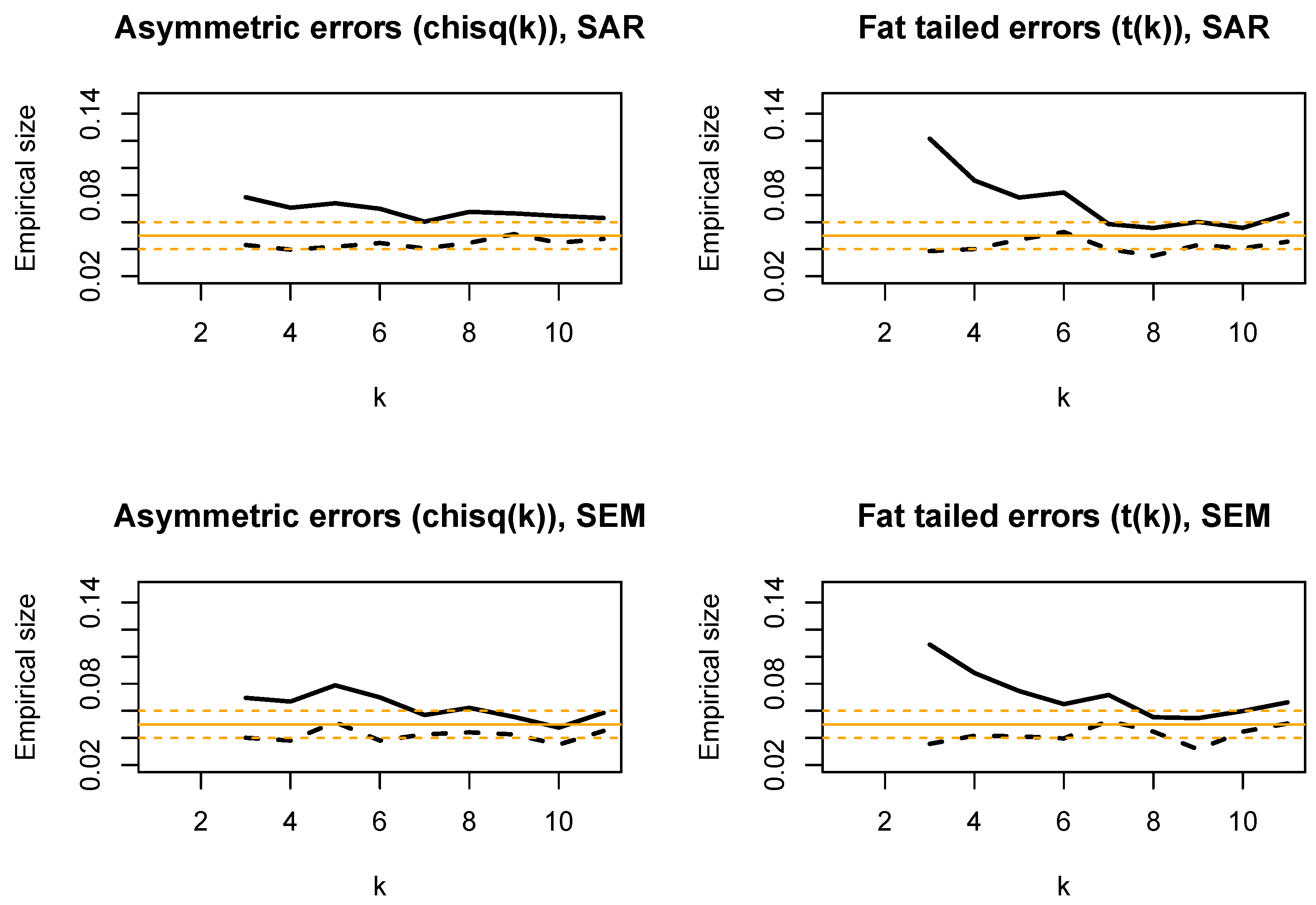
For these experiments, the DGP from Equations (1)–(3) is restricted to being either a SAR process with (top panels) or a SEM process with (bottom panels); no individual effects (); with , . Misspecification of the error distribution is likely to affect the empirical rejection frequency: hence, we focus on checking the test size, setting . A total of 2000 replications are performed; broken lines around the solid one at are 95% confidence bands for the empirical size ()
In Figure A1, we present the empirical size of the and tests as the degrees of freedom parameter k varies. The overrejecting behaviour of the is slightly more evident for strongly asymmetric errors (); more so in the presence of strong leptokurtosis (again, for ). The empirical size of the test does instead not seem to change (i.e., it remains only slightly underrejecting) with respect to the Normal errors case, for any k. Summing up, our limited experiment hints at both tests being satisfactorily sized under deviations from normality, exception made for the under rather extreme choices of the k parameter.
Figure A1.
Robustness check vs. error non-normality: empirical size of (solid line) and (broken line) for (asymmetric errors; left panels) or (fat-tailed errors; right panels) as ; DGP is a SAR process with (top panels) or a SEM process with (bottom panels); no individual effects (); with , . 2000 replications are performed; broken lines around the solid one at are 95% confidence bands for the empirical size ().
Appendix B. Software Howto
Currently, estimation of static spatial panels with serial correlation is only available in the open-source R environment [51] using available infrastructure from the plm and splm packages [31,54]. In particular, the Within function can be used for within-transforming the data, also directly inside the model formula to the spreml estimator
In the following, we illustrate operation through the Rice Farming example, recovering the results from the upper panel of Table 2 (spatial error model) and the lower panel (spatial lag + error) can be reproduced setting ‘lag=TRUE’.
> ## load packages
> library(plm)
> library(splm)
> ## load data and neighbourhood matrix
> data(RiceFarms, package="splm")
> data(riceww, package="splm")
> ## calculate dimensions
> n <- pdim(RiceFarms)$nT$n
> T. <- pdim(RiceFarms)$nT$T
A model with spatially and serially correlated errors but no individual effects (see Equation (6) above) is estimated:
> ## original model formula
> fm <- log(goutput) ~ log(seed)+log(urea)+phosphate+log(totlabor)+log(size)
> ## time-demeaned formula
> wfm <- Within(log(goutput)) ~ Within(log(seed)) + Within(log(urea)) +
+ Within(phosphate) + Within(log(totlabor)) + Within(log(size)) - 1
> ## estimate SEM+SR model (6) on demeaned data
> wmod <- spreml(wfm, data=RiceFarms, w=riceww, lag=FALSE, errors="semsr")
The necessary estimates and can then be fetched from the model summary, and the test statistic constructed as .
> ## time-demeaned formula
> wfm <- Within(log(goutput)) ~ Within(log(seed)) + Within(log(urea)) +
+ Within(phosphate) + Within(log(totlabor)) + Within(log(size)) - 1
> ## estimate SEM+SR model (6) on demeaned data
> wmod <- spreml(wfm, data=RiceFarms, w=riceww, lag=FALSE, errors="semsr")
> ## extract relevant elements from model summary
> psi <- summary(wmod)$ErrComp["psi", "Estimate"]
> SE.psi <- summary(wmod)$ErrComp["psi", "Std. Error"]
> ## perform testing
> ARfe <- (psi + 1/(T. - 1)) / SE.psi
> p.ARfe <- 2 * pnorm(abs(ARfe), lower.tail=FALSE)
> round(p.ARfe, 4)
[1] 0.002
There is currently no support for orthogonal decomposition of panel data in R. Therefore, performing the test requires sourcing an ad hoc function:
> Orthog <- function(x) {
+ Ft <- function(t) {
+ Aplus <- matrix(NA, ncol=t, nrow=t)
+ for(i in 1:(t-1)) Aplus[i,] <- -1/(t-i)
+ diag(Aplus) <- 1
+ Aplus[lower.tri(Aplus)] <- 0
+ Aplus <- Aplus[-dim(Aplus)[[1]], ]
+
+ a <- numeric(t-1)
+ for(i in 1:(t-1)) a[i] <- (t-i)/(t-i+1)
+ a <- diag(sqrt(a))
+
+ Ft <- a %*% Aplus
+ Ft
+ }
+ ortho <- function(x) Ft(length(x)) %*% x
+ res <- unlist(tapply(x, attr(x, "index")[[1]], ortho))
+ return(res)
+ }
and pre-transforming the data as shown below (a pooled model is estimated for conveniently preparing the data):
> ## OD-transformed formula
> ofm <- Orthog(log(goutput)) ~ Orthog(log(seed)) + Orthog(log(urea)) +
+ Orthog(phosphate) + Orthog(log(totlabor)) + Orthog(log(size)) - 1
> ## make orthog. transformed data and bespoke formula:
> ## preliminary estimation of pooled model
> omod <- plm(ofm, data=RiceFarms, m="p")
> ## make data.frame of transformed variables
> oX <- model.matrix(omod)
> oy <- pmodel.response(omod)
> odata <- as.data.frame(cbind(rep(1:n, each=T.-1), rep(1:(T.-1), n), oy, oX))
> dimnames(odata)[[2]] <- c("ind","tind","y","x1","x2","x3","x4","x5")
> ## make formula
> ofm <- y ~ x1 + x2 + x3 + x4 + x5
From here, one can then proceed as in the previous case. The auxiliary model is estimated, and the test statistic constructed as .
> omods <- try(spreml(ofm, data=odata, w=riceww,
+ lag=F, errors="semsr"))
> psio <- summary(omods)$ErrCompTable["psi", 1]
> SE.psio <- summary(omods)$ErrCompTable["psi", 2]
> ARod <- psio/SE.psio
> p.ARod <- 2 * pnorm(abs(ARod), lower.tail=FALSE)
> round(p.ARod, 4)
[1] 0.045
References
- Baltagi, B.; Song, S.; Jung, B.; Koh, W. Testing for serial correlation, spatial autocorrelation and random effects using panel data. J. Econom. 2007, 140, 5–51. [Google Scholar] [CrossRef]
- Debarsy, N.; Ertur, C. Testing for spatial autocorrelation in a fixed effects panel data model. Reg. Sci. Urban Econ. 2010, 40, 453–470. [Google Scholar] [CrossRef]
- Baltagi, B.H.; Yang, Z. Standardized LM tests for spatial error dependence in linear or panel regressions. Econom. J. 2013, 16, 103–134. [Google Scholar] [CrossRef]
- Baltagi, B.H.; Yang, Z. Heteroskedasticity and non-normality robust LM tests for spatial dependence. Reg. Sci. Urban Econ. 2013, 43, 725–739. [Google Scholar] [CrossRef]
- Badi, H.B.; Long, L. Testing for spatial lag and spatial error dependence in a fixed effects panel data model using double length artificial regressions. In Essays in Honor of man Ullah; Emerald Group Publishing Limited: Leeds, UK, 2016; pp. 67–84. [Google Scholar]
- Baltagi, B.H.; Liu, L. Random effects, fixed effects and Hausman’s test for the generalized mixed regressive spatial autoregressive panel data model. Econom. Rev. 2016, 35, 638–658. [Google Scholar] [CrossRef]
- Baltagi, B.H.; Kao, C.; Peng, B. On testing for sphericity with non-normality in a fixed effects panel data model. Stat. Probab. Lett. 2015, 98, 123–130. [Google Scholar] [CrossRef]
- Millo, G. Maximum likelihood estimation of spatially and serially correlated panels with random effects. Comput. Stat. Data Anal. 2014, 71, 914–933. [Google Scholar] [CrossRef]
- Lee, L.; Yu, J. A spatial dynamic panel data model with both time and individual fixed effects. Econom. Theory 2010, 26, 564–597. [Google Scholar] [CrossRef]
- Elhorst, J.P. Spatial Econometrics: From Cross-Sectional Data to Spatial Panels; Springer: Berlin/Heidelberg, Germany, 2014. [Google Scholar]
- Lee, L.f.; Yu, J. Identification of spatial Durbin panel models. J. Appl. Econom. 2016, 31, 133–162. [Google Scholar] [CrossRef]
- Yang, Z. Unified M-estimation of fixed-effects spatial dynamic models with short panels. J. Econom. 2018, 205, 423–447. [Google Scholar] [CrossRef]
- Lee, L.; Yu, J. Spatial panels: Random components versus fixed effects. Int. Econ. Rev. 2012, 53, 1369–1412. [Google Scholar] [CrossRef]
- Griffith, D.A. Some Remarks About the Future of Geographical Analysis: The Journal and the Sub-Discipline. Geogr. Anal. 2021, 53, 19–37. [Google Scholar] [CrossRef]
- Yang, Z. Joint tests for dynamic and spatial effects in short panels with fixed effects and heteroskedasticity. Empir. Econ. 2021, 60, 51–92. [Google Scholar] [CrossRef]
- Wooldridge, J. Econometric Analysis of Cross-Section and Panel Data; MIT Press: Cambridge, MA, USA, 2010. [Google Scholar]
- Lee, L.; Yu, J. Estimation of spatial autoregressive panel data models with fixed effects. J. Econom. 2010, 154, 165–185. [Google Scholar] [CrossRef]
- Elhorst, J. Serial and Spatial error correlation. Econ. Lett. 2008, 100, 422–424. [Google Scholar] [CrossRef]
- Montes-Rojas, G.V. Testing for random effects and serial correlation in spatial autoregressive models. J. Stat. Plan. Inference 2010, 140, 1013–1020. [Google Scholar] [CrossRef]
- Bouayad-Agha, S.; Turpin, N.; Védrine, L. Fostering the Potential Endogenous Development of European Regions: A Spatial Dynamic Panel Data Analysis of the Cohesion Policy on Regional Convergence over the Period 1980–2005; Technical report; TEPP: Bangkok, Thailand, 2012. [Google Scholar]
- Millo, G.; Carmeci, G. Non-life insurance consumption in Italy: A sub-regional panel data analysis. J. Geogr. Syst. 2011, 13, 273–298. [Google Scholar] [CrossRef]
- Millo, G.; Carmeci, G. A Subregional Panel Data Analysis of Life Insurance Consumption in Italy. J. Risk Insur. 2015, 82, 317–340. [Google Scholar] [CrossRef]
- Aravindakshan, A.; Peters, K.; Naik, P.A. Spatiotemporal allocation of advertising budgets. J. Mark. Res. 2012, 49, 1–14. [Google Scholar] [CrossRef]
- Lottmann, F. Explaining Regional Unemployment Differences in Germany: A Spatial Panel Data Analysis; SFB 649 Discussion Paper, No. 2012-026; Humboldt University of Berlin, Collaborative Research Center 649—Economic Risk: Berlin, Germany, 2012. [Google Scholar]
- Kunimitsu, Y.; Kudo, R.; Iizumi, T.; Yokozawa, M. Technological spillover in Japanese rice productivity under long-term climate change: Evidence from the spatial econometric model. Paddy Water Environ. 2015, 14, 131–144. [Google Scholar] [CrossRef]
- Lim-Wavde, K.; Kauffman, R.J.; Kam, T.S.; Dawson, G.S. Do grant funding and pro-environmental spillovers influence household hazardous waste collection? Appl. Geogr. 2019, 109, 102032. [Google Scholar] [CrossRef]
- Olivier, D.; Del Lo, G. Renewable energy drivers in France: A spatial econometric perspective. Reg. Stud. 2022, 56, 1633–1654. [Google Scholar] [CrossRef]
- Sadewo, E.; Hudalah, D.; Antipova, A.; Cheng, L.; Syabri, I. The role of urban transformation on inter-suburban commuting: Evidence from Jakarta metropolitan area, Indonesia. Urban Geogr. 2023, 44, 1628–1653. [Google Scholar] [CrossRef]
- Croissant, Y.; Millo, G. Panel Data Econometrics with R; Wiley: Hoboken, NJ, USA, 2019. [Google Scholar]
- Mátyás, L.; Sevestre, P. The econometrics of Panel Data: Fundamentals and Recent Developments in Theory and Practice; Springer Science & Business Media: Berlin/Heidelberg, Germany, 2008; Volume 46. [Google Scholar]
- Millo, G.; Piras, G. splm: Spatial panel data models in R. J. Stat. Softw. 2012, 47, 1–38. [Google Scholar] [CrossRef]
- Arellano, M.; Bover, O. Another look at the instrumental variable estimation of error-components models. J. Econom. 1995, 68, 29–51. [Google Scholar] [CrossRef]
- Elhorst, J. Specification and estimation of spatial panel data models. Int. Reg. Sci. Rev. 2003, 26, 244–268. [Google Scholar] [CrossRef]
- Anselin, L.; Le Gallo, J.; Jayet, H. Spatial Panel Econometrics. In Proceedings of the Econometrics of Panel Data, Fundamentals and Recent Developments in Theory and Practice, 3rd ed.; Matyas, L., Sevestre, P., Eds.; Springer: Berlin/Heidelberg, Germany, 2008; pp. 624–660. [Google Scholar]
- Lee, L.; Yu, J. Some recent developments in spatial panel data models. Reg. Sci. Urban Econ. 2010, 40, 255–271. [Google Scholar] [CrossRef]
- Arellano, M. Panel Data Econometrics; Oxford University Press: Oxford, UK, 2003. [Google Scholar]
- Drukker, D.M. Testing for serial correlation in linear panel-data models. Stata J. 2003, 3, 168–177. [Google Scholar] [CrossRef]
- Baltagi, B.H.; Li, Q. Testing AR (1) against MA (1) disturbances in an error component model. J. Econom. 1995, 68, 133–151. [Google Scholar] [CrossRef]
- Druska, V.; Horrace, W.C. Generalized moments estimation for spatial panel data: Indonesian rice farming. Am. J. Agric. Econ. 2004, 86, 185–198. [Google Scholar] [CrossRef]
- Baltagi, B. Econometric Analysis of Panel Data; John Wiley & Sons: Hoboken, NJ, USA, 2008; Volume 1. [Google Scholar]
- Croissant, Y. Ecdat: Data Sets for Econometrics; R Package Version 0.1-6; R Foundation for Statistical Computing: Vienna, Austria, 2010. [Google Scholar]
- Baltagi, B.H.; Levin, D. Cigarette taxation: Raising revenues and reducing consumption. Struct. Chang. Econ. Dyn. 1992, 3, 321–335. [Google Scholar] [CrossRef]
- Baltagi, B.H.; Griffin, J.M.; Xiong, W. To pool or not to pool: Homogeneous versus heterogeneous estimators applied to cigarette demand. Rev. Econ. Stat. 2000, 82, 117–126. [Google Scholar] [CrossRef]
- Baltagi, B.H.; Griffin, J.M. The econometrics of rational addiction: The case of cigarettes. J. Bus. Econ. Stat. 2001, 19, 449–454. [Google Scholar] [CrossRef]
- Baltagi, B.H.; Li, D. Prediction in the panel data model with spatial correlation. In Advances in Spatial Econometrics; Springer: Berlin/Heidelberg, Germany, 2004; pp. 283–295. [Google Scholar]
- Elhorst, J.P. Unconditional Maximum Likelihood Estimation of Linear and Log-Linear Dynamic Models for Spatial Panels. Geogr. Anal. 2005, 37, 85–106. [Google Scholar] [CrossRef]
- Elhorst, J.P. Matlab software for spatial panels. Int. Reg. Sci. Rev. 2012, 37, 389–405. [Google Scholar] [CrossRef]
- Kelejian, H.H.; Piras, G. An extension of Kelejian’s J-test for non-nested spatial models. Reg. Sci. Urban Econ. 2011, 41, 281–292. [Google Scholar] [CrossRef]
- Debarsy, N.; Ertur, C.; LeSage, J.P. Interpreting dynamic space–time panel data models. Stat. Methodol. 2012, 9, 158–171. [Google Scholar] [CrossRef]
- Kelejian, H.H.; Piras, G. Estimation of spatial models with endogenous weighting matrices, and an application to a demand model for cigarettes. Reg. Sci. Urban Econ. 2014, 46, 140–149. [Google Scholar] [CrossRef]
- R Development Core Team. R: A Language and Environment for Statistical Computing; R Foundation for Statistical Computing: Vienna, Austria, 2012; ISBN 3-900051-12-7. [Google Scholar]
- Shi, W.; Lee, L.f. Spatial dynamic panel data models with interactive fixed effects. J. Econom. 2017, 197, 323–347. [Google Scholar] [CrossRef]
- Long, J.S.; Ervin, L.H. Using heteroscedasticity consistent standard errors in the linear regression model. Am. Stat. 2000, 54, 217–224. [Google Scholar] [CrossRef]
- Croissant, Y.; Millo, G. Panel data econometrics in R: The plm package. J. Stat. Softw. 2008, 27, 1–43. [Google Scholar] [CrossRef]
Table 1.
Empirical size (bold) and power for the orthogonal deviations based test for , for and different T. is the individual effect variance, and , respectively, the SEM and SAR spatial parameters. 1000 replications.
Table 1.
Empirical size (bold) and power for the orthogonal deviations based test for , for and different T. is the individual effect variance, and , respectively, the SEM and SAR spatial parameters. 1000 replications.
| 0 | 0 | 0 | 0 | 1 | 1 | 1 | 1 | |||
|---|---|---|---|---|---|---|---|---|---|---|
| 0 | 0 | 0.5 | 0.5 | 0 | 0 | 0.5 | 0.5 | |||
| 0 | 0.5 | 0 | 0.5 | 0 | 0.5 | 0 | 0.5 | |||
| 4 | 0 | 0.062 | 0.061 | 0.064 | 0.066 | 0.068 | 0.069 | 0.063 | 0.061 | |
| 4 | 0.3 | 0.459 | 0.453 | 0.429 | 0.490 | 0.442 | 0.471 | 0.472 | 0.460 | |
| 4 | 0.8 | 0.993 | 0.990 | 0.996 | 0.994 | 0.995 | 0.991 | 0.993 | 0.996 | |
| 10 | 0 | 0.057 | 0.052 | 0.045 | 0.056 | 0.052 | 0.051 | 0.050 | 0.060 | |
| 10 | 0.3 | 0.998 | 0.999 | 0.997 | 0.998 | 0.999 | 0.999 | 0.998 | 0.998 | |
| 10 | 0.8 | 1.000 | 1.000 | 1.000 | 1.000 | 1.000 | 1.000 | 1.000 | 1.000 | |
| 15 | 0 | 0.067 | 0.052 | 0.041 | 0.054 | 0.044 | 0.055 | 0.054 | 0.051 | |
| 15 | 0.3 | 0.997 | 1.000 | 0.998 | 0.999 | 0.999 | 0.999 | 0.998 | 1.000 | |
| 15 | 0.8 | 1.000 | 1.000 | 1.000 | 1.000 | 1.000 | 1.000 | 1.000 | 1.000 |
Table 2.
Empirical size (bold) and power for the within transformation based test for , for and different T. is the individual effect variance, and , respectively, the SEM and SAR spatial parameters. 1000 replications.
Table 2.
Empirical size (bold) and power for the within transformation based test for , for and different T. is the individual effect variance, and , respectively, the SEM and SAR spatial parameters. 1000 replications.
| 0 | 0 | 0 | 0 | 1 | 1 | 1 | 1 | |||
|---|---|---|---|---|---|---|---|---|---|---|
| 0 | 0 | 0.5 | 0.5 | 0 | 0 | 0.5 | 0.5 | |||
| 0 | 0.5 | 0 | 0.5 | 0 | 0.5 | 0 | 0.5 | |||
| 4 | 0 | 0.030 | 0.024 | 0.040 | 0.032 | 0.020 | 0.034 | 0.034 | 0.042 | |
| 4 | 0.3 | 0.276 | 0.274 | 0.253 | 0.272 | 0.257 | 0.262 | 0.271 | 0.261 | |
| 4 | 0.8 | 0.964 | 0.956 | 0.962 | 0.957 | 0.965 | 0.962 | 0.966 | 0.961 | |
| 10 | 0 | 0.049 | 0.057 | 0.037 | 0.044 | 0.039 | 0.049 | 0.049 | 0.038 | |
| 10 | 0.3 | 1.000 | 0.999 | 0.998 | 0.999 | 1.000 | 1.000 | 0.998 | 0.998 | |
| 10 | 0.8 | 1.000 | 1.000 | 1.000 | 1.000 | 1.000 | 1.000 | 1.000 | 1.000 | |
| 15 | 0 | 0.045 | 0.045 | 0.038 | 0.048 | 0.037 | 0.042 | 0.046 | 0.051 | |
| 15 | 0.3 | 0.997 | 1.000 | 1.000 | 0.999 | 0.999 | 0.998 | 0.999 | 1.000 | |
| 15 | 0.8 | 1.000 | 1.000 | 1.000 | 1.000 | 1.000 | 1.000 | 1.000 | 1.000 |
Table 3.
Results and computing times (in seconds) for various serial correlation tests on the Italian Insurance dataset, SEM (upper panel) vs. full SAR + SEM specification (lower panel). is the joint test of Baltagi et al. [1], the conditional serial correlation test ibid.. and are the Likelihood Ratio and Wald tests equivalent to , from estimating the encompassing model: the estimated coefficient. and are the proposed tests. Computing times are obtained from R implementations on an AMD FX8320 desktop computer.
| SEM | |||||||
|---|---|---|---|---|---|---|---|
| Statistic | 703.1 | 22.251 | 35.07 | 5.618 | 0.52 | 9.356 | 4.212 |
| Distribution | z | - | z | z | |||
| p-value | 0 | 0 | 0 | 0 | - | 0 | 0 |
| Computing time | 0.05 | 4.84 | 14.76 | 10.20 | - | 0.68 | 0.42 |
| SAR + SEM | |||||||
| Statistic | - | - | 36.009 | 5.607 | 0.54 | 9.260 | 3.791 |
| Distribution | - | - | z | - | z | z | |
| p-value | - | - | 0 | 0 | - | 0 | 0.0002 |
| Computing time | - | - | 10.79 | 7.60 | - | 1.49 | 0.89 |
Table 4.
Results and computing times (in seconds) for various serial correlation tests on the Rice Farming dataset, SEM (upper panel) vs. full SAR + SEM specification (lower panel). is the joint test of Baltagi et al. [1], the conditional serial correlation test ibid.. and are the Likelihood Ratio and Wald tests equivalent to , from estimating the encompassing model: the estimated coefficient. and are the proposed tests. Computing times are obtained from R implementations on an AMD FX8320 desktop computer.
| SEM | |||||||
|---|---|---|---|---|---|---|---|
| Statistic | 1129.3 | 7.026 | 4.7306 | 2.129 | 0.087 | 2.005 | 3.085 |
| Distribution | z | - | z | z | |||
| p-value | 0 | 0.008 | 0.029 | 0.033 | - | 0.045 | 0.002 |
| Computing time | 0.15 | 5.41 | 15.40 | 9.95 | - | 1.72 | 2.46 |
| SAR + SEM | |||||||
| Statistic | - | - | 4.985 | 2.220 | 0.089 | 2.153 | 3.125 |
| Distribution | - | - | z | - | z | z | |
| p-value | - | - | 0.0256 | 0.0264 | - | 0.031 | 0.0017 |
| Computing time | - | - | 23.28 | 15.37 | - | 2.64 | 3.96 |
Table 5.
Results and computing times (in seconds) for various serial correlation tests, SEM (upper panel) vs. full SAR + SEM specification (lower panel). is the joint test of Baltagi et al. [1], the conditional serial correlation test ibid.. and are the Likelihood Ratio and Wald tests equivalent to , from estimating the encompassing model: the estimated coefficient. and are the proposed tests. Computing times are obtained from R implementations on an AMD FX8320 desktop computer.
| SEM | |||||||
|---|---|---|---|---|---|---|---|
| Statistic | 12,588.9 | 885.2 | 2034.7 | 286.0 | 0.98 | 86.6 | 89.7 |
| Distribution | z | - | z | z | |||
| p-value | 0 | 0 | 0 | 0 | - | 0 | 0 |
| Computing time | 0.23 | 16.41 | 27.96 | 15.81 | - | 2.94 | 2.74 |
| SAR + SEM | |||||||
| Statistic | - | - | 2031.5 | 293.6 | 0.98 | 90.3 | 95.4 |
| Distribution | - | - | z | - | z | z | |
| p-value | - | - | 0 | 0 | - | 0 | 0 |
| Computing time | - | - | 34.62 | 17.98 | - | 4.33 | 5.54 |
Disclaimer/Publisher’s Note: The statements, opinions and data contained in all publications are solely those of the individual author(s) and contributor(s) and not of MDPI and/or the editor(s). MDPI and/or the editor(s) disclaim responsibility for any injury to people or property resulting from any ideas, methods, instructions or products referred to in the content. |
© 2024 by the author. Licensee MDPI, Basel, Switzerland. This article is an open access article distributed under the terms and conditions of the Creative Commons Attribution (CC BY) license (https://creativecommons.org/licenses/by/4.0/).
Share and Cite
MDPI and ACS Style
Millo, G. An Ad Hoc Procedure for Testing Serial Correlation in Spatial Fixed-Effects Panels. Mathematics 2024, 12, 1475. https://doi.org/10.3390/math12101475
AMA Style
Millo G. An Ad Hoc Procedure for Testing Serial Correlation in Spatial Fixed-Effects Panels. Mathematics. 2024; 12(10):1475. https://doi.org/10.3390/math12101475
Chicago/Turabian StyleMillo, Giovanni. 2024. "An Ad Hoc Procedure for Testing Serial Correlation in Spatial Fixed-Effects Panels" Mathematics 12, no. 10: 1475. https://doi.org/10.3390/math12101475
Note that from the first issue of 2016, this journal uses article numbers instead of page numbers. See further details here.