The Strictly Dissipative Condition of Continuous-Time Markovian Jump Systems with Uncertain Transition Rates

Abstract

This study addresses the problem of strictly dissipative stabilization for continuous-time Markovian jump systems (MJSs) with external disturbances and generally uncertain transition rates that contain completely unknown transition rates and their bound values. A stabilization condition is obtained to guarantee strict dissipativity for the MJSs with partial knowledge in terms of the transition rates. To reduce the conservativity of the proposed condition, we used a boundary condition related to the bounds of the transition rate with slack variables. Finally, two simulation results are presented to describe the feasibility of the proposed controller.

1. Introduction

Over the past decades, there has been increasing interest in Markovian jump systems (MJSs), which effectively represent practical systems with unexpected variations [1,2,3,4,5,6]. MJSs have been studied by many researchers using stability analysis [7], controller synthesis [8,9,10], and filter design [11,12,13]. These results have contributed to the extensive application of MJSs, including power systems [14,15,16], economic systems [17,18,19,20], and manufacturing systems [21]. Because the MJSs are constructed using a group of linear systems influenced by a Markov process, the knowledge of transition probabilities for the jumping process is an important challenge. However, it is difficult to accurately determine the transition probabilities in many practical applications, leading to limitations in modeling various practical systems.

Recently, to overcome this difficulty, studies on the stabilization of MJSs with transition probabilities that contain uncertainty have attracted considerable interest concerning control theory [22,23]. Specifically, because the transition probabilities in continuous-time MJSs depend on the transition rates, many researchers have focused on how to handle uncertain transition rates for the stabilization of continuous-time MJSs. Ref. [24] proposed a state observer for MJSs with time-varying delays, where the transition probabilities were assumed to change in a polytope with vertices. Refs. [25,26] employed the boundary values of the transition rates for the controller synthesis of MJSs. Although these approaches consider the uncertainty of the transition rates, it is difficult to precisely estimate their bounds in practical systems. To address this challenge, the stabilization method of MJSs with state delays was investigated in [27] based on the partial known and unknown transition rates. However, similar to other results on the analysis and synthesis of MJSs, Ref. [27] developed a method assuming that some transition rates are precisely known. More recently, Ref. [28] introduced a new structure for the transition rates, generally uncertain transition rates (GUTRs), which contain bounds of the uncertainties of the known and unknown transition rates. The method reported in Ref. [28] has piqued the interest of researchers [29,30] concerning the stabilization problem of MJSs. These results all focus on the uncertainties of the transition rates, but there is no consideration of external disturbances. Hence, it is vital to consider the uncertain transition rates and disturbances concerning realistic system stability analysis and synthesis problems.

In contrast, the dissipativity theory has become an important approach to studying control systems concerning the stabilization problem [31,32,33,34]. Dissipativity is characterized by the input–output energy concerning the stored energy in the system and supplied energy from outside the system [35]. Furthermore, the dissipativity performance can be applied to the $H_{\infty }$ and passivity performance [36]. Based on these properties, many researchers have focused on the dissipativity problem in the stabilization of interconnected systems, switched systems, and Markovian jump systems [37,38,39,40]. Ref. [37] introduced a framework for dissipativity for switched systems, employing multiple storage functions and supply rates. Ref. [38] proposed a stabilization method for Markovian jump fuzzy systems with asynchronous controllers. Ref. [39] studied dissipative filter design for singular MJSs with hybrid transition rates. Ref. [40] proposed an asynchronous dissipative controller for semi-MJSs using distribution of the sojourn time. To the best of our knowledge, the dissipativity control for continuous-time MJSs with GUTRs has not yet been analyzed, thus forming the motivation of our study.

This study attempted to design a strictly dissipative controller for MJSs with external disturbances and GUTRs that can represent all possible cases: (1) known transition rates, (2) unknown transition rates, and (3) known bounds of the transition rates but unknown exact transition rates. Following is a list of the specific contributions of this study.

• In practice, it is necessary to consider the uncertainties in the transition rates and disturbances from outside the system. Therefore, to address this issue, we proposed a strictly dissipative controller for MJSs with external disturbances and GUTRs that have not yet been introduced.
• To design the proposed controller, stabilization conditions were formulated using linear matrix inequalities (LMIs) with various matrix variables. Considering the strict dissipativity and GUTRs, these conditions may be conservative because of the lack of information about the transition rates. Therefore, this study introduced an appropriate weighting approach to reduce the conservatism of the stabilization condition using the known bounds of the transition rates with slack variables.

Two simulation results show the effectiveness of the proposed stabilization condition.

This paper is divided into five sections. Section 2 describes the proposed MJSs and their preliminaries. The design process of the strictly dissipative controller for MJSs with external disturbances and GUTRs is shown in Section 3. Simulation examples are presented in Section 4 to demonstrate the feasibility of the proposed method. Finally, Section 5 presents the conclusions of this study.

$\mathsf{Notation:}$ The notation $A>B$ indicates that $A-B$ is a positive definite for any matrix. ${\mathbb{R}}^n$ represents the n-dimensional Euclidean space. $(\ast )$ denotes an ellipsis for symmetry-induced terms in symmetric block matrices. Furthermore, $\mathbf{He}\left(A\right)=A+A^T$ for any matrix A. $\mathbf{E}\left[A\right]$ is the expectation of A. $L_2[0,\infty )$ means the space of square-summable sequences over $[0,\infty )$.

2. System Description

Let us consider a continuous-time MJS:

$$\begin{array}{c}\dot{x}\left(t\right)=A\left(r\left(t\right)\right)x\left(t\right)+B\left(r\left(t\right)\right)u\left(t\right)+G\left(r\left(t\right)\right)\omega \left(t\right),\hfill \\ z\left(t\right)=E\left(r\right(t\left)\right)x\left(t\right)+F\left(r\right(t\left)\right)u\left(t\right)+J\left(r\right(t\left)\right)\omega \left(t\right),\hfill \end{array}$$

(1)

where $x\left(t\right)\in {\mathbb{R}}^n$ denotes the state, $u\left(t\right)\in {\mathbb{R}}^m$ denotes the input, $\omega \left(t\right)\in {\mathbb{R}}^{n_{\omega }}$ denotes the external disturbance belonging to $L_2[0,\infty )$, and $z\left(t\right)\in {\mathbb{R}}^{n_z}$ denotes the performance output. Here, $r\left(t\right)\in \mathcal{D}=\{1, 2,\cdots ,\mathcal{M}\}$ represents a continuous-time Markov jump. To represent the Markov jump from mode i to j at time $t+h$, the transition probability is defined as:

$$\begin{array}{c}\hfill P(r(t+h)=j|r\left(t\right)=i)=\left\{\begin{array}{cc}{\pi }_{ij}h+o\left(h\right)\hfill & \mathrm{if} i\ne j\hfill \\ 1+{\pi }_{ii}h+o\left(h\right)\hfill & \mathrm{if} i=j,\hfill \end{array}\right.\end{array}$$

(2)

where ${\pi }_{ij}$ is the transition rate with ${\pi }_{ij}\ge 0$, $i\ne j$; ${\pi }_{ii}=-{\sum }_{j\in \mathcal{D},i\ne j}{\pi }_{ij}$, $h>0$ is the transition time interval; and ${\displaystyle \underset{h\to 0}{lim}\frac{o\left(h\right)}{h}=0}$.

Then, the transition rate matrix $\Pi$, which has unknown or bounded transition rates, can be described as:

$$\begin{array}{c}\hfill \Pi =\left[\begin{array}{cccc}[{\pi }_{11}^{min}, {\pi }_{11}^{max}]& \times & \cdots & [{\pi }_{1\mathcal{M}}^{min}, {\pi }_{1\mathcal{M}}^{max}]\\ \times & \times & \cdots & ⋮\\ ⋮& ⋮& \ddots & ⋮\\ {\pi }_{\mathcal{M}1}^{min}, {\pi }_{\mathcal{M}1}^{max}]& \times & \cdots & [{\pi }_{\mathcal{M}\mathcal{M}}^{min}, {\pi }_{\mathcal{M}\mathcal{M}}^{max}]\end{array}\right],\end{array}$$

(3)

where ${\pi }_{ij}^{min}$ and ${\pi }_{ij}^{max}$ denote the minimum and maximum bounds of ${\pi }_{ij}$; × is the completely unknown transition rate; and the notation ⋱ signifies that the diagonal terms of the matrix are successively populated with the values ${\pi }_{ij}^{min}$ and ${\pi }_{ij}^{max}$, where the indices i and j increase simultaneously by 1. The above transition rate matrix can represent all possible transition rates that can contain unknown, bounded, or known transition rates for ${\pi }_{ij}^{min}={\pi }_{ij}^{max}$. This is called a GUTR. Therefore, the transition rate can be rewritten as:

$$\begin{array}{c}\hfill {\pi }_{ij}={\tilde{\pi }}_{ij}+\delta {\pi }_{ij},\end{array}$$

(4)

where ${\tilde{\pi }}_{ij}=({\pi }_{ij}^{max}+{\pi }_{ij}^{min})/2$, $\delta {\pi }_{ij}\in [-{\Delta }_{ij},{\Delta }_{ij}]$, ${\Delta }_{ij}=({\pi }_{ij}^{max}-{\pi }_{ij}^{min})/2$.

Subsequently, depending on the transition rates, we can define the following two mode sets:

$$\begin{array}{cc}\hfill {\mathcal{D}}_i& =\left\{j\right|{\pi }_{ij}\in [{\pi }_{ij}^{min},{\pi }_{ij}^{max}] \mathrm{are} \mathrm{unknown} \mathrm{but} \mathrm{bounded} \mathrm{for} i\},\hfill \end{array}$$

(5)

$$\begin{array}{cc}\hfill {\tilde{\mathcal{D}}}_i& =\left\{j\right|{\pi }_{ij} \mathrm{are} \mathrm{completely} \mathrm{unknown} \mathrm{for} i\},\hfill \end{array}$$

(6)

where $\mathcal{D}={\mathcal{D}}_i\cup {\tilde{\mathcal{D}}}_i$. ${\mathcal{D}}_i$ refers to the collection of column indices in the ith row of matrix $\Pi$, where the transition rates have known bounds, while ${\tilde{\mathcal{D}}}_i$ denotes the collection of column indices with unknown transition rates. Here, an element of ${\tilde{\mathcal{D}}}_i$ is given by ${\kappa }_l$, where $1\le l\le L$ and $1\le L\le \mathcal{M}$.

For convenience, when $r\left(t\right)=i$, System (1) can be deduced as

$$\begin{array}{c}\dot{x}\left(t\right)=A_{i}x\left(t\right)+B_{i}u\left(t\right)+G_i\omega \left(t\right),\hfill \\ z\left(t\right)=E_{i}x\left(t\right)+F_{i}u\left(t\right)+J_i\omega \left(t\right).\hfill \end{array}$$

(7)

Definition 1

([41]). The system is stochastically stable when $\omega \left(t\right)\equiv 0$ if the following holds:

$$\begin{array}{c}\hfill \underset{t\to \infty }{lim}\mathbf{E}\left[{\int }_0^t{\parallel x\left(\tau \right)\parallel }^2\mathrm{d}\tau \right]<\infty .\end{array}$$

(8)

Definition 2

([42]). Based on dissipativity theory, the quadratic energy supply rate can be described as:

$$\begin{array}{c}\hfill \mathcal{R}(z\left(t\right),\omega \left(t\right))={\left[\begin{array}{c}z\left(t\right)\\ \omega \left(t\right)\end{array}\right]}^{\mathrm{T}}\left[\begin{array}{cc}Q& S\\ S^{\mathrm{T}}& R\end{array}\right]\left[\begin{array}{c}z\left(t\right)\\ \omega \left(t\right)\end{array}\right],\end{array}$$

(9)

where $Q=-{\tilde{Q}}^{\mathrm{T}}\tilde{Q}<0$, S, and $R=R^{\mathrm{T}}$ are known real matrices. For a scalar $\beta >0$ and $T>0$, the following condition holds when $x\left(0\right)=0$:

$$\begin{array}{c}\hfill {\int }_0^T\mathbf{E}\left[\mathcal{R}\left(z\right(t),\omega (t\left)\right)\right]\mathrm{d}t>\beta {\int }_0^T{\omega }^{\mathrm{T}}\left(t\right)\omega \left(t\right)\mathrm{d}t.\end{array}$$

(10)

Then, (1) is a strictly $(Q,S,R)$-β-dissipative system, where β represents the dissipative performance.

This study attempted to design a controller that guarantees stochastic stability for System (1) when $\omega \left(t\right)\equiv 0$ and strictly $(Q,S,R)$-$\beta$-dissipativity when $x\left(0\right)=0$.

3. Main Result

This section focuses on the design of the dissipative stabilization condition for System (7) with GUTRs. First, we introduce the stability and strictly dissipative conditions for the open-loop system of System (7) with fully known transition rates. Then, the stabilization condition is introduced for strictly $(Q,S,R)$-$\beta$-dissipativity with GUTRs.

3.1. Stability Analysis for the Open-Loop System with Known Transition Rates

The following lemma provides the stochastic stability condition for the open-loop condition of System (7) based on Definition 1.

Lemma 1

([43]). The MJS is stochastically stable when $u\left(t\right)=0$ and $\omega \left(t\right)=0$ iff there exists matrix $P_i>0$ ∀$i\in \mathcal{D}$, such that

$$\begin{array}{c}\hfill \mathbf{H}\mathbf{e}\left(P_i{A}_i\right)+\sum _{j=1}^{\mathcal{M}}{\pi }_{ij}{P}_j<0.\end{array}$$

(11)

The following lemma gives the strict $(Q,S,R)$-$\beta$-dissipativity condition for the open-loop system of (7).

Lemma 2.

The continuous-time MJS is strictly $(Q,S,R)$-β-dissipative when $u\left(t\right)=0$ if matrix $P_i>0$ for all $i\in \mathcal{D}$ and a given scalar β exists, such that

$$\begin{array}{c}\hfill \left[\begin{array}{ccc}{\displaystyle \mathbf{H}\mathbf{e}\left(P_i{A}_i\right)+\sum _{j=1}^{\mathcal{M}}{\pi }_{ij}{P}_i}& (\ast )& (\ast )\\ G_i^{\mathrm{T}}{P}_i+S^{\mathrm{T}}{E}_i& -\mathbf{H}\mathbf{e}\left(S^{\mathrm{T}}{J}_i\right)-R+\beta I& (\ast )\\ \tilde{Q}{E}_i& \tilde{Q}{J}_i& -I\end{array}\right]<0.\end{array}$$

(12)

Proof. 

Based on the proof of Lemma 1, we consider a Lyapunov function, $V\left(t\right)=x^{\mathrm{T}}\left(t\right)P\left(r\left(t\right)\right)x\left(t\right)$$=V\left(x\right(t),r(t\left)\right)$, where $P\left(r\right(t\left)\right)>0$. The infinitesimal operator $\mathcal{A}$ of $V\left(x\right(t\left)\right)$ is then obtained as follows:

$$\begin{array}{c}\hfill \mathcal{A}V\left(t\right)=\underset{h\to 0}{lim}\frac{\mathbf{E}\left[V\right(x(t+h),r(t+h)=j\left)\right|x\left(t\right),r\left(t\right)=i]-V(x\left(t\right),r\left(t\right)=i)}{h}.\end{array}$$

Using the definition of transition probability in (2), $\mathcal{A}V\left(t\right)$ is derived as follows:

$$\begin{array}{cc}\mathcal{A}V\left(t\right)\hfill & =\underset{h\to 0}{lim}\left(\sum _{j=1}^{\mathcal{M}}{\pi }_{ij}V(x(t+h),j)+\frac{V\left(x\right(t+h),i)-V\left(x\right(t),i)}{h}\right)\hfill \\ & =\underset{h\to 0}{lim}\frac{V\left(x\right(t+h),i)-V\left(x\right(t),i)}{h}+\sum _{j=1}^{\mathcal{M}}{\pi }_{ij}V(x(t+h),j)\hfill \\ & =x^{\mathrm{T}}\left(t\right)\{\mathbf{H}\mathbf{e}\left(P_i{A}_i\right)+\sum _{j=1}^{\mathcal{M}}{\pi }_{ij}{P}_j\}x\left(t\right).\hfill \end{array}$$

(13)

Therefore, (11) ensures that

$$\begin{array}{c}\hfill \mathcal{A}V\left(t\right)=x^{\mathrm{T}}\left(t\right){\Psi }_{i}x\left(t\right)={\eta }^{\mathrm{T}}\left(t\right){\widehat{\Psi }}_i\eta \left(t\right)<0,\end{array}$$

(14)

where

$$\begin{array}{c}{\Psi }_i=\mathbf{H}\mathbf{e}\left(P_i{A}_i\right)+\sum _{j=1}^{\mathcal{M}}{\pi }_{ij}{P}_j,\eta \left(t\right)={\left[\begin{array}{cc}x\left(t\right)& \omega \left(t\right)\end{array}\right]}^{\mathrm{T}},{\widehat{\Psi }}_i=\mathbf{H}\mathbf{e}\left({\widehat{P}}_i{\widehat{A}}_i\right)+\sum _{j=1}^{\mathcal{M}}{\pi }_{ij}{\widehat{P}}_j,\hfill \\ {\widehat{A}}_i=\left[\begin{array}{cc}{A}_i& G_i\\ 0& 0\end{array}\right],{\widehat{P}}_i=\left[\begin{array}{cc}{P}_i& 0\\ 0& 0\end{array}\right].\hfill \end{array}$$

From (9) and (14), it follows that

$$\begin{array}{c}\mathcal{A}V\left(t\right)-\mathcal{R}\left(t\right)+\beta {\omega }^{\mathrm{T}}\left(t\right)\omega \left(t\right)\hfill \\ ={\eta }^{\mathrm{T}}\left(t\right)\left({\widehat{\Psi }}_i-\left[\begin{array}{cc}{E}_i^{\mathrm{T}}Q{E}_i& (\ast )\\ J_i^{\mathrm{T}}Q{E}_i+S^{\mathrm{T}}{E}_i& J_i^{\mathrm{T}}Q{J}_i+\mathbf{H}\mathbf{e}\left(S^{\mathrm{T}}{J}_i\right)+R+\beta I\end{array}\right]\right)\eta \left(t\right)\hfill \\ ={\eta }^{\mathrm{T}}\left(t\right)\left({\widehat{\Psi }}_i-\left[\begin{array}{cc}0& (\ast )\\ S^{\mathrm{T}}{E}_i& +\mathbf{H}\mathbf{e}\left(S^{\mathrm{T}}{J}_i\right)+R+\beta I\end{array}\right]+\left[\begin{array}{c}{\left(\tilde{Q}{E}_i\right)}^{\mathrm{T}}\\ {\left(\tilde{Q}{J}_i\right)}^{\mathrm{T}}\end{array}\right]\left[\begin{array}{cc}\tilde{Q}{E}_i& \tilde{Q}{J}_i\end{array}\right]\right)\eta \left(t\right).\hfill \end{array}$$

(15)

Applying the Schur complement to (12), we obtain the following condition:

$$\begin{array}{c}\hfill {\widehat{\Psi }}_i-\left[\begin{array}{cc}0& (\ast )\\ S^{\mathrm{T}}{E}_i& +\mathbf{H}\mathbf{e}\left(S^{\mathrm{T}}{J}_i\right)+R+\beta I\end{array}\right]+\left[\begin{array}{c}{\left(\tilde{Q}{E}_i\right)}^{\mathrm{T}}\\ {\left(\tilde{Q}{J}_i\right)}^{\mathrm{T}}\end{array}\right]\left[\begin{array}{cc}\tilde{Q}{E}_i& \tilde{Q}{J}_i\end{array}\right]<0.\end{array}$$

Accordingly, if condition (12) is satisfied, then

$$\begin{array}{c}\hfill \mathbf{E}[\mathcal{A}V\left(t\right)-\mathcal{R}\left(t\right)+\beta {\omega }^{\mathrm{T}}\left(t\right)\omega \left(t\right)]<0.\end{array}$$

(16)

By integral transformation, (16) leads to

$$\begin{array}{c}\hfill \mathbf{E}\left[{\int }_0^T\mathcal{A}V\left(t\right)\mathrm{d}t\right]-{\int }_0^T\mathbf{E}\left[\mathcal{R}\left(t\right)\right]\mathrm{d}t+{\int }_0^T\beta {\omega }^{\mathrm{T}}\left(t\right)\omega \left(t\right)\mathrm{d}t<0.\end{array}$$

(17)

By Dynkin’s formula [44], the above inequality is rewritten as

$$\begin{array}{c}\hfill \mathbf{E}\left[V\left(T\right)\right]-V\left(0\right)-{\int }_0^T\mathbf{E}\left[\mathcal{R}\left(t\right)\right]\mathrm{d}t+{\int }_0^T\beta {\omega }^{\mathrm{T}}\left(t\right)\omega \left(t\right)\mathrm{d}t<0.\end{array}$$

(18)

When $x\left(0\right)=0$, we have

$$\begin{array}{c}\hfill {\int }_0^T\beta {\omega }^{\mathrm{T}}\left(t\right)\omega \left(t\right)\mathrm{d}t-{\int }_0^T\mathbf{E}\left[\mathcal{R}\left(t\right)\right]\mathrm{d}t<-\mathbf{E}\left[V\left(T\right)\right]<0.\end{array}$$

(19)

Therefore, Condition (10) is satisfied by (19), which means that the open-loop system of (7) is strictly $(Q,S,R)$-$\beta$-dissipative based on Definition 2. □

3.2. Controller Synthesis with GUTRs

Let us consider the following mode-dependent controller:

$$\begin{array}{c}\hfill u\left(t\right)=K\left(r_t\right)x\left(t\right),\end{array}$$

(20)

where $K\left(r_t\right)\in {\mathbb{R}}^{n\times m}$ denotes the mode-dependent control gain. The proposed controller is designed to ensure stability in systems modeled as continuous-time MJSs even in the presence of uncertain transition rates. It also minimizes the impact of external disturbances on the output. Subsequently, the closed-loop system in (7) with (20) is given as follows:

$$\begin{array}{c}\hfill \dot{x}\left(t\right)=A_i^{c}x\left(t\right)+G_i\omega \left(t\right),\\ \hfill z\left(t\right)=E_i^{c}x\left(t\right)+J_i\omega \left(t\right),\end{array}$$

(21)

where $A_i^c=A_i+B_i{K}_i$ and $E_i^c=E_i+F_i{K}_i$.

The following theorem provides the stabilization condition for strictly $(Q,S,R)$-$\beta$-dissipativity, and the condition is formulated in the form of LMIs.

Theorem 1.

For a given positive scalar β and $i\in \mathcal{D}$, if matrices ${\overline{P}}_i>0$, ${\overline{S}}_i>0$ and ${\overline{U}}_{ij}>0$, and ${\Lambda }_{ij}$ exist such that

$$\begin{array}{c}{\Lambda }_{ij}+{\Lambda }_{ij}^{\mathrm{T}}>0,\hspace{1em}j\in {\mathcal{D}}_i\hfill \end{array}$$

(22)

$$\begin{array}{c}{\overline{P}}_i-{\overline{S}}_i>0,\hspace{1em}j\in {\tilde{\mathcal{D}}}_i,i=j\hfill \end{array}$$

(23)

$$\begin{array}{c}\left[\begin{array}{cc}{\overline{S}}_i& (\ast )\\ {\overline{P}}_i& {\overline{P}}_j\end{array}\right]>0,\hspace{1em}j\in {\tilde{\mathcal{D}}}_i,i\ne j\hfill \end{array}$$

(24)

$$\begin{array}{c}\left[\begin{array}{cc}{\overline{S}}_i+{\overline{U}}_{ij}& (\ast )\\ {\overline{P}}_i& {\overline{P}}_j\end{array}\right]>0,\hspace{1em}j\in {\mathcal{D}}_i\hfill \end{array}$$

(25)

$$\begin{array}{c}\left[\begin{array}{cc}{M}_i^c+{ϵ}_i{\pi }_{ii}^{max}{\overline{P}}_i& (\ast )\\ {\mathcal{N}}_i& -\overline{\mathcal{P}}\end{array}\right]<0,\hfill \end{array}$$

(26)

$$\begin{array}{c}\left[\begin{array}{cc}{\tilde{M}}_i^c& (\ast )\\ {\mathcal{N}}_{i}E& -\overline{\mathcal{P}}\end{array}\right]<0,\hfill \end{array}$$

(27)

where

$$\begin{array}{cc}\hfill M_i^c& =\mathbf{H}\mathbf{e}(A_i{\overline{P}}_i+B_i{\overline{K}}_i)-\sum _{j\in {\mathcal{D}}_i}{\pi }_{ij}^{max}{\overline{S}}_i+\sum _{j\in {\mathcal{D}}_i}2{\Delta }_{ij}({\overline{U}}_{ij}+\mathbf{H}\mathbf{e}\left({\Lambda }_i\right)),\hfill \\ \hfill {\overline{K}}_i& =K_i{\overline{P}}_i,\hfill \\ \hfill {\mathcal{N}}_i& ={\left[\begin{array}{ccc}\sqrt{{\pi }_{i{\kappa }_1}^{max}}{\overline{P}}_i& \cdots & \sqrt{{\pi }_{i{\kappa }_L}^{max}}{\overline{P}}_i\end{array}\right]}^{\mathrm{T}},\hfill \\ \hfill \overline{\mathcal{P}}& =\mathit{diag}\left\{\begin{array}{ccc}{\overline{P}}_{{\kappa }_1},& \cdots ,& {\overline{P}}_{{\kappa }_L}\end{array}\right\},\hfill \\ \hfill {\tilde{M}}_i^c& =\left[\begin{array}{ccc}{(1,1)}^c& (\ast )& (\ast )\\ G_i^{\mathrm{T}}-S^{\mathrm{T}}(E_i{\overline{P}}_i+F_i{\overline{K}}_i)& -\mathbf{H}\mathbf{e}\left(S^{\mathrm{T}}{J}_i\right)-R+\beta I& (\ast )\\ \tilde{Q}(E_i{\overline{P}}_i+F_i{\overline{K}}_i)& \tilde{Q}{J}_i& -I\end{array}\right],\hfill \\ \hfill {(1,1)}^c& =\mathbf{H}\mathbf{e}(A_i{\overline{P}}_i+B_i{\overline{K}}_i)+\sum _{j\in {\mathcal{D}}_i}2{\Delta }_{ij}{\overline{U}}_{ij}-\sum _{j\in {\mathcal{D}}_i}{\pi }_{ij}^{max}{\overline{S}}_i+ϵ{\pi }_{ii}^{max}{\overline{P}}_i,\hfill \\ \hfill {ϵ}_i& =\left\{\begin{array}{cc}0\hfill & \mathit{if} i\notin {\mathcal{D}}_i\hfill \\ 1\hfill & \mathit{if} i\in {\mathcal{D}}_i\hfill \end{array}\right.,\hfill \\ \hfill \mathcal{I}& =\left[\begin{array}{ccc}I& 0& 0\end{array}\right]\in {\mathbb{R}}^{n\times (n+n_{\omega }+n_z)},\hfill \end{array}$$

then the closed-loop system is stochastically stable and strictly $(Q,S,R)$-β-dissipative. Furthermore, the proposed controller is obtained as $u\left(t\right)=K_{i}x\left(t\right)$, where $K_i={\overline{K}}_i{\overline{P}}_i^{-1}$.

Proof. 

First, we provide the proof of the stochastic stabilization conditions. From the closed-loop system in (21) and Lemma 1, we obtain the following condition:

$$\begin{array}{c}\hfill \mathbf{H}\mathbf{e}\left(P_i{A}_i^c\right)+\sum _{j=1}^{\mathcal{M}}{\pi }_{ij}{P}_j<0.\end{array}$$

(28)

Using the property of the transition rate and matrix $S_i>0$ satisfying ${\sum }_{j=1}^{\mathcal{M}}{\pi }_{ij}{S}_i=0$, the following condition is derived:

$$\begin{array}{c}\mathbf{H}\mathbf{e}\left(P_i{A}_i^c\right)+\sum _{j\in {\mathcal{D}}_i}{\pi }_{ij}{P}_j+\sum _{j\in {\tilde{\mathcal{D}}}_i}{\pi }_{ij}{P}_j+\sum _{j=1}^{\mathcal{M}}{\pi }_{ij}{S}_i\hfill \\ =\mathbf{H}\mathbf{e}\left(P_i{A}_i^c\right)+\sum _{j\in {\mathcal{D}}_i}{\pi }_{ij}{T}_{ij}+\sum _{j\in {\tilde{\mathcal{D}}}_i}{\pi }_{ij}{T}_{ij}<0,\hfill \end{array}$$

(29)

where $T_{ij}=P_j-S_i$.

For $i,j\in \mathcal{D}$, if the following inequality holds:

$$\begin{array}{c}\hfill T_{ij}>0\hspace{1em}\mathrm{if} i=j,\end{array}$$

(30)

$$\begin{array}{c}\hfill T_{ij}<0\hspace{1em}\mathrm{if} i\ne j,\end{array}$$

(31)

then Condition (29) holds as

$$\begin{array}{c}\hfill \mathbf{H}\mathbf{e}\left(P_i{A}_i^c\right)+\sum _{j\in {\mathcal{D}}_i}{\pi }_{ij}{T}_{ij}<0.\end{array}$$

(32)

Based on the definition of the GUTR in (4), Condition (32) can be rewritten as

$$\begin{array}{c}\hfill \mathbf{H}\mathbf{e}\left(P_i{A}_i^c\right)+\sum _{j\in {\mathcal{D}}_i}({\tilde{\pi }}_{ij}-{\Delta }_{ij})T_{ij}+\sum _{j\in {\mathcal{D}}_i}(\delta {\pi }_{ij}+{\Delta }_{ij})T_{ij}<0.\end{array}$$

(33)

Using only the known information on the transition rate, we adopt the upper bound of the second and last terms on the left-hand side of (33). It thus follows that

$$\begin{array}{c}\sum _{j\in {\mathcal{D}}_i}({\tilde{\pi }}_{ij}-{\Delta }_{ij})T_{ij}\le \sum _{j\in {\mathcal{D}}_i}{\pi }_{ij}^{max}{T}_{ij},\hfill \end{array}$$

(34)

$$\begin{array}{c}\sum _{j\in {\mathcal{D}}_i}(\delta {\pi }_{ij}+{\Delta }_{ij})T_{ij}\le \sum _{j\in {\mathcal{D}}_i}2{\Delta }_{ij}{T}_{ij}\le \sum _{j\in {\mathcal{D}}_i}2{\Delta }_{ij}{U}_{ij},\hfill \end{array}$$

(35)

where $U_{ij}>0$ and

$$\begin{array}{c}\hfill T_{ij}-U_{ij}<0.\end{array}$$

(36)

Then, we can obtain the sufficient condition of (33) as follows:

$$\begin{array}{c}\hfill \mathbf{H}\mathbf{e}\left(P_i{A}_i^c\right)+\sum _{j\in {\mathcal{D}}_i}{\pi }_{ij}^{max}{T}_{ij}+\sum _{j\in {\mathcal{D}}_i}2{\Delta }_{ij}{U}_{ij}<0.\end{array}$$

(37)

Multiplying both sides of the above inequality by $P_i^{-1}$ gives

$$\begin{array}{c}\hfill \mathbf{H}\mathbf{e}\left(A_i^c{\overline{P}}_i\right)+\sum _{j\in {\mathcal{D}}_i}{\pi }_{ij}^{max}{\overline{T}}_{ij}+\sum _{j\in {\mathcal{D}}_i}2{\Delta }_{ij}{\overline{U}}_{ij}<0,\end{array}$$

(38)

where ${\overline{P}}_i=P_i^{-1}$, ${\overline{T}}_{ij}={\overline{P}}_i{P}_j{\overline{P}}_i-{\overline{S}}_i$, ${\overline{S}}_i={\overline{P}}_i{S}_i{\overline{P}}_i$ and ${\overline{U}}_{ij}={\overline{P}}_i{U}_{ij}{\overline{P}}_i$.

Next, due to (22),

$$\begin{array}{c}\hfill \sum _{j\in {\mathcal{D}}_i}({\pi }_{ij}^{max}-{\pi }_{ij}^{min})\mathbf{H}\mathbf{e}\left({\Lambda }_{ij}\right)\ge 0,\end{array}$$

(39)

which is a weighting method with slack variables ${\Lambda }_{ij}$ that can reduce the conservatism of (38).

Using the $\mathcal{S}$-procedure, (38), subject to (39), is formulated in terms of

$$\begin{array}{c}\hfill M_i^c+ϵ{\pi }_{ii}^{max}{\overline{P}}_i+\sum _{j\in {\mathcal{D}}_i,i\ne j}{\pi }_{ij}^{max}{\overline{P}}_i{P}_j{\overline{P}}_i<0.\end{array}$$

(40)

Then, Condition (40) is transformed into

$$\begin{array}{c}\hfill M_i^c+ϵ{\pi }_{ii}^{max}{\overline{P}}_i-{\mathcal{N}}_i^T(-\mathcal{P}){\mathcal{N}}_i<0,\end{array}$$

(41)

where $\mathcal{P}=\mathrm{diag}\left\{\begin{array}{c}{P}_{{\kappa }_1},\cdots ,P_{{\kappa }_L}\end{array}\right\}$.

Using the Schur complement, it can be demonstrated that (41) implies (26). From the above proof, we can obtain the stochastic stabilization condition of System (21).

Second, for the proof of the strictly $(Q,S,R)$-$\beta$-dissipative condition using Lemma 2, we can obtain the sufficient condition of (12) for the closed-loop system in (21):

$$\begin{array}{c}\hfill \left[\begin{array}{ccc}{\displaystyle \mathbf{H}\mathbf{e}\left(P_i{A}_i^c\right)+\sum _{j\in {\mathcal{D}}_k}{\pi }_{ij}^{max}{T}_{ij}+\sum _{j\in {\mathcal{D}}_k}2{\Delta }_{ij}{U}_{ij}}& (\ast )& (\ast )\\ G_i^{\mathrm{T}}{P}_i+S^{\mathrm{T}}{E}_i^c& -\mathbf{H}\mathbf{e}\left(S^{\mathrm{T}}{J}_i\right)-R+\beta I& (\ast )\\ \tilde{Q}{E}_i^c& \tilde{Q}{J}_i& -I\end{array}\right]<0,\end{array}$$

(42)

because ${\displaystyle \mathbf{H}\mathbf{e}\left(P_i{A}_i^c\right)+{\sum }_{j=1}^{\mathcal{M}}{\pi }_{ij}{P}_i<\mathbf{H}\mathbf{e}\left(P_i{A}_i^c\right)+\sum _{j\in {\mathcal{D}}_k}{\pi }_{ij}^{max}{T}_{ij}+\sum _{j\in {\mathcal{D}}_k}2{\Delta }_{ij}{U}_{ij}}$, as shown in (34) and (35).

Multiplying both sides of (42) with $\mathrm{diag}\left\{\begin{array}{c}{\overline{P}}_i,I,I\end{array}\right\}$ yields

$$\begin{array}{c}\hfill {\tilde{M}}_i^c-{\left({\mathcal{N}}_i\mathcal{I}\right)}^{\mathrm{T}}(-\mathcal{P})\left({\mathcal{N}}_i\mathcal{I}\right)<0.\end{array}$$

(43)

Then, using the Schur complement, it can be shown that (43) implies (27). Furthermore, from Condition (30), the LMI condition in (23) can be obtained by

$$\begin{array}{c}\hfill {\overline{P}}_i(P_i-S_i){\overline{P}}_i<0.\end{array}$$

(44)

The LMI conditions in (24) and (25) can be acquired by

$$\begin{array}{c}{\overline{P}}_i(P_j-S_i){\overline{P}}_i>0,\hfill \end{array}$$

(45)

$$\begin{array}{c}{\overline{P}}_i(P_j-S_i-U_{ij}){\overline{P}}_i<0,\hfill \end{array}$$

(46)

and by using the Schur complement from Conditions (31) and (36), respectively. Therefore, the closed-loop system in (21) is strictly $(Q,S,R)$-$\beta$-dissipative according to Definition 2. □

Remark 1.

The Conditions (30) and (31) maintain the stabilization condition’s inequality while removing the unknown transition rates from the condition. This approach allows for a more generalized stabilization criterion that handles uncertainties in transition rates without compromising the condition’s integrity. By employing the inequalities, we effectively decouple the stabilization condition from the specific values of the transition rates, thereby enhancing the applicability of our findings to systems with partially or completely unknown transition dynamics.

In Theorem 1, the following optimization problem provides the optimal dissipative performance bound $\beta$:

$$\begin{array}{c}min -\beta \hfill \\ \mathrm{s}.\mathrm{t}. \left(22\right)-\left(27\right).\hfill \end{array}$$

(47)

Moreover, Theorem 1 can be extended to achieve ${\mathcal{H}}_{\infty }$ and passivity performance as in the following cases:

• ${\mathcal{H}}_{\infty }$ performance: $\tilde{Q}=I$, $S=0$, and $R=\gamma I+\beta I$,
• Passivity performance: $Q=0$, $S=I$, and $R=2\beta I$.

Remark 2.

Note that the proposed theorem is based on the LMI approach. To solve the optimization problem based on this theorem, we used the Robust Control Toolbox in MATLAB 2022. Therefore, all the computations to solve the optimization problem are off-line, which can be solved using Toolbox. When the LMIs have a solution, the controller gains and optimal dissipative performance bounds are obtained.

4. Examples

In this section, numerical and practical examples are presented to verify the effectiveness of the proposed approach.

4.1. Example 1

Consider the following numerical example, as used in [22]:

$$\begin{array}{c}{A}_1=\left[\begin{array}{cc}0.35& -7.30\\ 1.48& 0.81\end{array}\right], A_2=\left[\begin{array}{cc}0.89& -3.11\\ 1.48& 0.21\end{array}\right],\hfill \\ A_3=\left[\begin{array}{cc}-0.11& -0.85\\ 2.31& -0.10\end{array}\right], A_4=\left[\begin{array}{cc}-0.17& -1.48\\ 1.59& -0.27\end{array}\right],\hfill \\ B_1=\left[\begin{array}{c}0.57\\ 1.23\end{array}\right], B_2=\left[\begin{array}{c}0.78\\ -0.49\end{array}\right], B_3=\left[\begin{array}{c}1.34\\ 0.39\end{array}\right], B_4=\left[\begin{array}{c}-0.38\\ 1.07\end{array}\right],\hfill \\ G_1=\left[\begin{array}{c}0.5\\ 0.1\end{array}\right], G_2=\left[\begin{array}{c}0.15\\ 0.0\end{array}\right], G_3=\left[\begin{array}{c}0.0\\ 0.4\end{array}\right], G_4=\left[\begin{array}{c}0.2\\ 0.3\end{array}\right],\hfill \\ E_1=\left[\begin{array}{cc}0.0& -0.1\end{array}\right], E_2=\left[\begin{array}{cc}0.1& 0.0\end{array}\right], E_3=\left[\begin{array}{cc}0.0& 0.1\end{array}\right], E_4=\left[\begin{array}{cc}0.1& 0.0\end{array}\right],\hfill \\ F_1=F_2=F_3=F_4=0, J_1=J_2=J_3=J_4=0,\hfill \\ Q=-1, S=0.1, R=1.\hfill \end{array}$$

The transition rate matrix $\Pi$ is:

$$\begin{array}{c}\hfill \Pi =\left[\begin{array}{cccc}[-1.5,-1.2]& [0.1,0.3]& \times & \times \\ \times & \times & [0.2,0.4]& [0.2,0.4]\\ [0.5,0.7]& \times & [-1.6,-1.4]& \times \\ [0.3,0.5]& \times & \times & \times \end{array}\right].\end{array}$$

From the above transition matrix, we can obtain the following sets for the measurability of ${\pi }_{ij}$:

$$\begin{array}{c}{\mathcal{D}}_1=\{1,2\},{\tilde{\mathcal{D}}}_1=\{3,4\},{\mathcal{D}}_2=\{3,4\},{\tilde{\mathcal{D}}}_2=\{1,2\},\hfill \\ {\mathcal{D}}_3=\{1,3\},{\tilde{\mathcal{D}}}_3=\{2,4\},{\mathcal{D}}_4=\left\{1\right\},{\tilde{\mathcal{D}}}_4=\{2,3,4\}.\hfill \end{array}$$

Based on the above system parameters, Figure 1a shows the state trajectories for this example, which means that this system is in an unstable open-loop condition with $u\left(t\right)=0$.

By solving the proposed conditions in Theorem 1, we can obtain the optimal dissipative performance, $\beta =0.9932$, and the proposed controller gains are

$$\begin{array}{c}{K}_1=\left[\begin{array}{cc}5.8609& -10.690\end{array}\right], K_2=\left[\begin{array}{cc}-7.5336& 4.0370\end{array}\right],\hfill \\ K_3=\left[\begin{array}{cc}-2.2120& -4.1430\end{array}\right], K_4=\left[\begin{array}{cc}3.2756& -4.2008\end{array}\right].\hfill \end{array}$$

Based on these gains, Figure 1b shows the state trajectories of the closed-loop system and the mode evolution with $x\left(0\right)={\left[\begin{array}{c}0.4,-1.2\end{array}\right]}^{\mathrm{T}}$ and $\omega \left(t\right)=0$. Figure 2 presents the state trajectories with the mode evolution and control input under $x\left(0\right)={[0, 0]}^{\mathrm{T}}$ and $\omega \left(t\right)=e^{-0.2t}$. From these figures, the state trajectories converge to zero as the time increases. This verifies that the proposed method guarantees the strict $(Q,S,R)$-$\beta$-dissipativity and stochastic stability of the MJS with external disturbances and GUTRs.

4.2. Example 2

Consider the following mass-spring-damper mechanical system [45]:

$$\begin{array}{c}\hfill M\ddot{y}\left(t\right)+D\dot{y}\left(t\right)+V\left(t\right)y\left(t\right)=(1+c{\dot{y}}^3\left(t\right))u\left(t\right)+\omega \left(t\right),\end{array}$$

(48)

where $y\left(t\right)$ is the position of the mass, $u\left(t\right)$ is the input force, $\omega \left(t\right)$ is the external disturbance, M is the mass, and D is the viscous damping. Here, $V\left(t\right)=V\left(r_t\right)$ is the time-varying stiffness, which is defined as

$$\begin{array}{c}\hfill V\left(r_t\right)=\left\{\begin{array}{cc}0.5\hfill & \mathrm{if} r_t=1\hfill \\ 1.81\hfill & \mathrm{if} r_t=2\hfill \end{array}\right..\end{array}$$

Here, we assume that $M=1$, $D=1$, $c=0$, $x\left(t\right)={\left[\begin{array}{cc}\dot{y}\left(t\right)& y\left(t\right)\end{array}\right]}^{\mathrm{T}}$, and $z\left(t\right)={\left[\begin{array}{cc}y\left(t\right)& u\left(t\right)\end{array}\right]}^{\mathrm{T}}$. Using the above parameters, System (49) can be constructed as the following MJS:

$$\begin{array}{c}\dot{x}\left(t\right)=A\left(r\left(t\right)\right)x\left(t\right)+B\left(r\left(t\right)\right)u\left(t\right)+G\left(r\left(t\right)\right)\omega \left(t\right),\hfill \\ z\left(t\right)=E\left(r\right(t\left)\right)x\left(t\right)+F\left(r\right(t\left)\right)u\left(t\right)+J\left(r\right(t\left)\right)\omega \left(t\right),\hfill \end{array}$$

(49)

where

$$\begin{array}{c}{A}_1=\left[\begin{array}{cc}-1& -0.5\\ 1& 0\end{array}\right],A_2=\left[\begin{array}{cc}-1& -1.81\\ 1& 0\end{array}\right],B_1=\left[\begin{array}{c}1\\ 0\end{array}\right],B_2=\left[\begin{array}{c}1\\ 0\end{array}\right],\hfill \\ G_1=G_2=\left[\begin{array}{c}1\\ 0\end{array}\right],E_1=E_2=\left[\begin{array}{cc}0& 1\\ 0& 0\end{array}\right],F_1=F_2=\left[\begin{array}{c}0\\ 1\end{array}\right],J_1=J_2=J_3=J_4=0.\hfill \end{array}$$

Table 1 lists the corresponding transition matrices for different transition rates. Here, in Cases 2 and 3, the transition matrices contain unknown transition rates for each mode, representing the asynchrony between each mode in (49). Table 2 lists the optimal performance values of the different transition matrices in Table 1. The performance values are obtained using the following conditions:

• Dissipativity performance: $Q=\left[\begin{array}{cc}-1& 0\\ 0& -1\end{array}\right],S=\left[\begin{array}{c}0.1\\ 0.1\end{array}\right],R=1$,
• ${\mathcal{H}}_{\infty }$ performance: $Q=\left[\begin{array}{cc}-1& 0\\ 0& -1\end{array}\right]$, $S=0$, $R=(\gamma +\beta )\left[\begin{array}{cc}1& 0\\ 0& 1\end{array}\right]$.

Table 2 demonstrates that these performance values deteriorate with the degree of asynchronous intensification in each case. Specifically, for Case 3, the following control gains can be obtained by solving the optimization problem in (47) for strictly $(Q,S,R)$-$\beta$-dissipativity:

$$\begin{array}{c}\hfill K_1=\left[\begin{array}{cc}-1.8518& -1.4186\end{array}\right], K_2=\left[\begin{array}{cc}-2.0079& -1.5633\end{array}\right].\end{array}$$

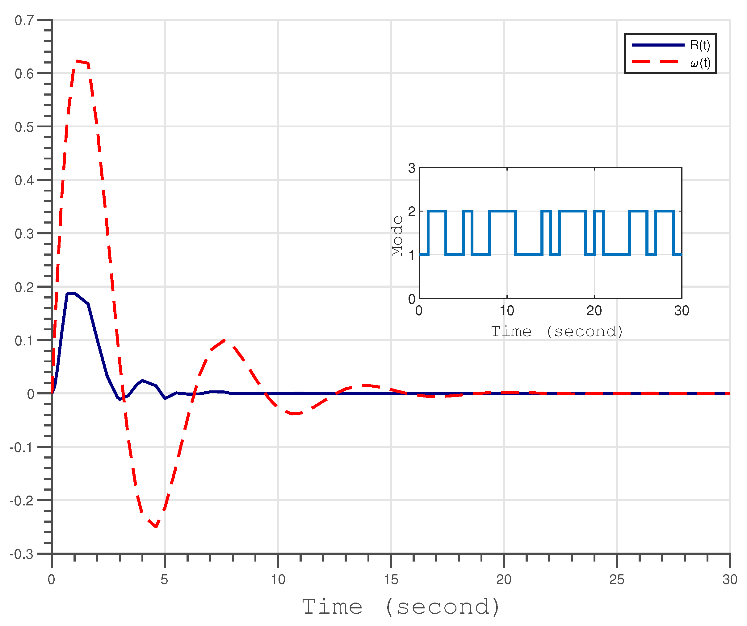
Based on the proposed controller employing the above gains, we obtained the state trajectories and mode evolution under $x\left(0\right)=[-1, -0.5]$ and $\omega \left(t\right)=e^{-0.3t}sin\left(t\right)$, as shown in Figure 3a. Figure 3b represents the control input. Thus, Figure 3 shows that the controller stochastically stabilizes the MJS with external disturbances and GUTRs.

Furthermore, Figure 4 shows the energy supply rate $\mathcal{R}\left(t\right)$ and external disturbance $\omega \left(t\right)$. From Figure 4, the dissipativity performance value can be obtained by $\frac{{\int }_0^{30}\mathbf{E}\left[\mathcal{R}\left(z\right(t),\omega (t\left)\right)\right]\mathrm{d}t}{{\int }_0^{30}{\omega }^{\mathrm{T}}\left(t\right)\omega \left(t\right)\mathrm{d}t}$ = 0.3631. Therefore, (49) satisfies the strict $(Q,S,R)$-$\beta$-dissipativity because the calculated performance value is larger than the performance bound $\beta =0.1379$.

Table 1. Transition matrix $\Pi$.

Case 1	Case 2	Case 3
$\left[\begin{array}{cc}-3& 3\\ 4& -4\end{array}\right]$	$\left[\begin{array}{cc}-3& 3\\ [3,5]& \times \end{array}\right]$	$\left[\begin{array}{cc}\times & \times \\ [3,5]& \times \end{array}\right]$

Table 1. Transition matrix $\Pi$.

Case 1	Case 2	Case 3
$\left[\begin{array}{cc}-3& 3\\ 4& -4\end{array}\right]$	$\left[\begin{array}{cc}-3& 3\\ [3,5]& \times \end{array}\right]$	$\left[\begin{array}{cc}\times & \times \\ [3,5]& \times \end{array}\right]$

Table 2. Comparison of the optimal $\beta$ with different transition rates.

Performance	Case 1	Case 2	Case 3
Dissipativity ($\beta$)	0.5277	0.4340	0.1379
$H_{\infty }$ ($\gamma$)	0.4722	0.5660	0.8620

Table 2. Comparison of the optimal $\beta$ with different transition rates.

Performance	Case 1	Case 2	Case 3
Dissipativity ($\beta$)	0.5277	0.4340	0.1379
$H_{\infty }$ ($\gamma$)	0.4722	0.5660	0.8620

5. Conclusions

This study addressed the strictly dissipative control problem of continuous-time MJSs with external disturbances and GUTRs. The stabilization condition was derived with the mode-dependent Lyapunov function, formulated as an LMI, to guarantee stochastic stability and strict dissipativity. Furthermore, to reduce the conservatism of the derived conditions, we introduced an appropriate weighting method related to the bounds of the transition rate with slack variables. Finally, the effectiveness of the proposed approach was verified using two examples.

References

- Elliott, R.J.; Aggoun, L.; Moore, J.B. Hidden Markov Models: Estimation and Control; Springer Science & Business Media: Berlin/Heidelberg, Germany, 2008; Volume 29. [Google Scholar]
- Shi, P.; Li, F. A survey on Markovian jump systems: Modeling and design. Int. J. Control. Autom. Syst. 2015, 13, 1–16. [Google Scholar] [CrossRef]
- Anbazhagan, N.; Joshi, G.P.; Suganya, R.; Amutha, S.; Vinitha, V.; Shrestha, B. Queueing-Inventory System for Two Commodities with Optional Demands of Customers and MAP Arrivals. Mathematics 2022, 10, 1801. [Google Scholar] [CrossRef]
- Dudin, A.; Dudina, O.; Dudin, S.; Samouylov, K. Analysis of Single-Server Multi-Class Queue with Unreliable Service, Batch Correlated Arrivals, Customers Impatience, and Dynamical Change of Priorities. Mathematics 2021, 9, 1257. [Google Scholar] [CrossRef]
- Barron, Y. A stochastic card balance management problem with continuous and batch-type bilateral transactions. Oper. Res. Perspect. 2023, 10, 100274. [Google Scholar] [CrossRef]
- Barron, Y. Integrating Replenishment Policy and Maintenance Services in a Stochastic Inventory System with Bilateral Movements. Mathematics 2023, 11, 864. [Google Scholar] [CrossRef]
- Costa, O.L.V.; Fragoso, M.D. Stability Results for Discrete-Time Linear Systems with Markovian Jumping Parameters. J. Math. Anal. Appl. 1993, 179, 154–178. [Google Scholar] [CrossRef]
- Sworder, D. Feedback control of a class of linear systems with jump parameters. IEEE Trans. Autom. Control 1969, 14, 9–14. [Google Scholar] [CrossRef]
- Ji, Y.; Chizeck, H. Controllability, stabilizability, and continuous-time Markovian jump linear quadratic control. IEEE Trans. Autom. Control 1990, 35, 777–788. [Google Scholar] [CrossRef]
- Feng, X.; Loparo, K. Stability of linear Markovian jump systems. In Proceedings of the 29th IEEE Conference on Decision and Control, Honolulu, HI, USA, 5–7 December 1990; Volume 3, pp. 1408–1413. [Google Scholar] [CrossRef]
- Zhang, L.; Boukas, E.K. Mode-dependent H∞ filtering for discrete-time Markovian jump linear systems with partly unknown transition probabilities. Automatica 2009, 45, 1462–1467. [Google Scholar] [CrossRef]
- Park, C.E.; Kwon, N.K.; Park, P. Optimal H∞ filtering for singular Markovian jump systems. Syst. Control Lett. 2018, 118, 22–28. [Google Scholar] [CrossRef]
- Park, C.E.; Kwon, N.K.; Park, I.S.; Park, P. H∞ filtering for singular Markovian jump systems with partly unknown transition rates. Automatica 2019, 109, 108528. [Google Scholar] [CrossRef]
- Ugrinovskii, V.; Pota, H.R. Decentralized control of power systems via robust control of uncertain Markov jump parameter systems. Int. J. Control 2005, 78, 662–677. [Google Scholar] [CrossRef]
- Li, L.; Ugrinovskii, V.A.; Orsi, R. Decentralized robust control of uncertain Markov jump parameter systems via output feedback. Automatica 2007, 43, 1932–1944. [Google Scholar] [CrossRef]
- Kazemy, A.; Hajatipour, M. Event-triggered load frequency control of Markovian jump interconnected power systems under denial-of-service attacks. Int. J. Electr. Power Energy Syst. 2021, 133, 107250. [Google Scholar] [CrossRef]
- Cogley, T.W. Optimal monetary policy under uncertainty: A Markov jump-linear-quadratic approach-Commentary. Fed. Reserve Bank St. Louis Rev. 2008, 90, 295–300. [Google Scholar]
- Blair, W., Jr.; Sworder, D. Feedback control of a class of linear discrete systems with jump parameters and quadratic cost criteria. Int. J. Control 1975, 21, 833–841. [Google Scholar] [CrossRef]
- Breuer, L. A quintuple law for Markov additive processes with phase-type jumps. J. Appl. Probab. 2010, 47, 441–458. [Google Scholar] [CrossRef]
- Chakravarthy, S.R.; Rao, B.M. Queuing-Inventory Models with MAP Demands and Random Replenishment Opportunities. Mathematics 2021, 9, 1092. [Google Scholar] [CrossRef]
- Martinelli, F. Optimality of a Two-Threshold Feedback Control for a Manufacturing System with a Production Dependent Failure Rate. IEEE Trans. Autom. Control 2007, 52, 1937–1942. [Google Scholar] [CrossRef]
- Shin, J.; Park, B.Y. H∞ Control of Markovian Jump Systems with Incomplete Knowledge of Transition Probabilities. Int. J. Control. Autom. Syst. 2019, 17, 2474–2481. [Google Scholar] [CrossRef]
- Wang, B.; Zhu, Q. Stability analysis of discrete-time semi-Markov jump linear systems with partly unknown semi-Markov kernel. Syst. Control Lett. 2020, 140, 104688. [Google Scholar] [CrossRef]
- Li, S.; Xiang, Z.; Lin, H.; Karimi, H.R. State estimation on positive Markovian jump systems with time-varying delay and uncertain transition probabilities. Inf. Sci. 2016, 369, 251–266. [Google Scholar] [CrossRef]
- Shi, P.; Boukas, E.K. H∞ Control for Markovian Jumping Linear Systems with Parametric Uncertainty. J. Optim. Theory Appl. 1997, 95, 75–99. [Google Scholar] [CrossRef]
- Xiong, J.; Lam, J. Robust H2 control of Markovian jump systems with uncertain switching probabilities. Int. J. Syst. Sci. 2009, 40, 255–265. [Google Scholar] [CrossRef]
- Zhang, L.; Boukas, E.K.; Lam, J. Analysis and Synthesis of Markov Jump Linear Systems With Time-Varying Delays and Partially Known Transition Probabilities. IEEE Trans. Autom. Control 2008, 53, 2458–2464. [Google Scholar] [CrossRef]
- Guo, Y.; Wang, Z. Stability of Markovian jump systems with generally uncertain transition rates. J. Frankl. Inst. 2013, 350, 2826–2836. [Google Scholar] [CrossRef]
- Li, X.; Zhang, W.; Lu, D. Stability and stabilization analysis of Markovian jump systems with generally bounded transition probabilities. J. Frankl. Inst. 2020, 357, 8416–8434. [Google Scholar] [CrossRef]
- Lee, W.I.; Park, B.Y. Stabilization of Markovian Jump Systems With Quantized Input and Generally Uncertain Transition Rates. IEEE Access 2021, 9, 83499–83506. [Google Scholar] [CrossRef]
- Willems, J.C. Dissipative dynamical systems part I: General theory. Arch. Ration. Mech. Anal. 1972, 45, 321–351. [Google Scholar] [CrossRef]
- Hill, D.J.; Moylan, P.J. Dissipative Dynamical Systems: Basic Input-Output and State Properties. J. Frankl. Inst. 1980, 309, 327–357. [Google Scholar] [CrossRef]
- Pakshin, P.V. Dissipativity of diffusion Itô processes with Markovain switching and problems of robust stabilization. Autom. Remote Control 2007, 68, 1502–1518. [Google Scholar] [CrossRef]
- Pakshin, P.V. Exponential dissipativeness of the random-structure diffusion processes and problems of robust stabilization. Autom. Remote Control 2007, 68, 1852–1870. [Google Scholar] [CrossRef]
- Willems, J.C. Dissipative Dynamical Systems. Eur. J. Control 2007, 13, 134–151. [Google Scholar] [CrossRef]
- Kim, S.H. Dissipative control of Markovian jump fuzzy systems under nonhomogeneity and asynchronism. Nonlinear Dyn. 2019, 97, 629–646. [Google Scholar] [CrossRef]
- Zhao, J.; Hill, D.J. Dissipativity Theory for Switched Systems. IEEE Trans. Autom. Control 2008, 53, 941–953. [Google Scholar] [CrossRef]
- Dong, S.; Wu, Z.G.; Su, H.; Shi, P.; Karimi, H.R. Asynchronous Control of Continuous-Time Nonlinear Markov Jump Systems Subject to Strict Dissipativity. IEEE Trans. Autom. Control 2019, 64, 1250–1256. [Google Scholar] [CrossRef]
- Tian, Y.; Wang, Z. Dissipative filtering for singular Markovian jump systems with generally hybrid transition rates. Appl. Math. Comput. 2021, 411, 126492. [Google Scholar] [CrossRef]
- Nguyen, N.H.A.; Kim, S.H. Asynchronous dissipative control design for semi-Markovian jump systems with uncertain probability distribution functions of sojourn-time. Appl. Math. Comput. 2021, 397, 125921. [Google Scholar] [CrossRef]
- Xie, S.; Xie, L.; De Souza, C.E. Robust dissipative control for linear systems with dissipative uncertainty. Int. J. Control 1998, 70, 169–191. [Google Scholar] [CrossRef]
- Xie, S.; Xie, L. Robust dissipative control for linear systems with dissipative uncertainty and nonlinear perturbation. Syst. Control Lett. 1997, 29, 255–268. [Google Scholar] [CrossRef]
- De Farias, D.P.; Geromel, J.C.; Do Val, J.B.; Costa, O.L. Output feedback control of Markov jump linear systems in continuous-time. IEEE Trans. Autom. Control 2000, 45, 944–949. [Google Scholar] [CrossRef]
- Oksendal, B. Stochastic Differential Equations: An Introduction with Applications; Springer Science & Business Media: Berlin/Heidelberg, Germany, 2013. [Google Scholar]
- Wu, H.N. Reliable Robust H∞ Fuzzy Control for Uncertain Nonlinear Systems With Markovian Jumping Actuator Faults. J. Dyn. Syst. Meas. Control 2007, 129, 252–261. [Google Scholar] [CrossRef]
Figure 1.
State trajectories for the (a) open-loop and (b) closed-loop systems under and .
Figure 2.
(a) State trajectories and (b) input trajectories for the closed-loop system under and .
Figure 3.
(a) State trajectories and (b) input trajectories under and .
Figure 4.
The comparison of the energy supply rate and for .
Disclaimer/Publisher’s Note: The statements, opinions and data contained in all publications are solely those of the individual author(s) and contributor(s) and not of MDPI and/or the editor(s). MDPI and/or the editor(s) disclaim responsibility for any injury to people or property resulting from any ideas, methods, instructions or products referred to in the content. |
© 2024 by the authors. Licensee MDPI, Basel, Switzerland. This article is an open access article distributed under the terms and conditions of the Creative Commons Attribution (CC BY) license (https://creativecommons.org/licenses/by/4.0/).
Share and Cite
MDPI and ACS Style
Lee, W.; Shin, J.; Park, B. The Strictly Dissipative Condition of Continuous-Time Markovian Jump Systems with Uncertain Transition Rates. Mathematics 2024, 12, 639. https://doi.org/10.3390/math12050639
AMA Style
Lee W, Shin J, Park B. The Strictly Dissipative Condition of Continuous-Time Markovian Jump Systems with Uncertain Transition Rates. Mathematics. 2024; 12(5):639. https://doi.org/10.3390/math12050639
Chicago/Turabian StyleLee, WonIl, JaeWook Shin, and BumYong Park. 2024. "The Strictly Dissipative Condition of Continuous-Time Markovian Jump Systems with Uncertain Transition Rates" Mathematics 12, no. 5: 639. https://doi.org/10.3390/math12050639
Note that from the first issue of 2016, this journal uses article numbers instead of page numbers. See further details here.