
Study on Temperature Cascade ELM Inversion Method for 110 kV Single-Core Cable Intermediate Joints

1
Guangdong Zhongshan Power Supply Bureau of China Southern Power Grid Co., Ltd., Zhongshan 528400, China
2
School of Electrical Engineering and Automation, Wuhan University, Wuhan 430072, China
*
Author to whom correspondence should be addressed.
Processes 2024, 12(5), 966; https://doi.org/10.3390/pr12050966
Submission received: 9 April 2024
/
Revised: 1 May 2024
/
Accepted: 5 May 2024
/
Published: 9 May 2024
(This article belongs to the Section Energy Systems)
Abstract
:The accurate calculation of the hotspot temperature of the cable intermediate joint can effectively guarantee the safe operation of the transmission and distribution network. This paper addresses the limitations of the current method of estimating hotspot temperature solely from surface temperature measurements. Specifically, we focus on a 110 kV single-core cable as our subject of study. We started by establishing a simulation model for the temperature field at the intermediate joint to generate data samples. Subsequently, the NCA (neighborhood component analysis) algorithm was employed to select the optimal measurement points on the cable’s surface. This allowed determination of the quantity and location of characteristic points. Finally, we developed a cascading inversion model, which consists of a radial inversion model and an axial inversion model, based on the extreme learning machine algorithm. The example results show that the mean squared error of hotspot temperature obtained by cascade inversion and direct inversion is 6.95 and 24.71, respectively, indicating that cascade inversion can effectively improve the inversion accuracy.
1. Introduction
As a basic component of the power system transmission and distribution network, the insulation health status of power cables is directly related to the safe and stable operation of the power supply system. Due to the complexity of the process, material dispersion, and concentration of electrical stress during cable production and installation, the intermediate joints are prone to insulation breakdown under the action of electrical and thermal stresses, which becomes the weakest point in the insulation of the cable system [1,2]. To ensure the safe and stable operation of the transmission and distribution network, the temperature of the cable intermediate joints must be accurately calculated.
At present, the methods used for simulating the temperature field of cable bodies and intermediate joints mainly include analytical methods and numerical computation methods. The former often relies on the IEC 60853 standard [3], combined with thermal path models [4,5], comparative analysis [6], etc., to study the temperature rise issues in cables. However, these methods yield conservatively calculated results that may not fully meet the actual engineering demands for the power supply capacity of electrical cables. On the other hand, numerical computation methods can simulate the complex operating environments of cables and produce more accurate temperature field simulation results. Researchers like Tang Ke and others [7] have used the finite element method (FEM) to simulate the temperature fields of single cables and three-phase cables, fitting the temperature difference functions between the two to enhance simulation accuracy. Pu Lu and others [8] have established an electromagnetic–thermal coupled simulation model for the intermediate joints of single-core cables, studying the relationships between surface temperature and core temperature of the joint under various environmental temperatures, load currents, and operational conditions, which affirmed the effectiveness of this method. Zhao Xuefeng and others [9] have applied finite element numerical algorithms to simulate soil-direct-buried cable bodies and joints, analyzing the impacts of temperature-dependent conductor resistance and moisture migration on the temperature and current-carrying capacity of intermediate joints. Gao Yunpeng and others [10] have established simplified transient thermal path models for cable joints and proposed an inversion algorithm for the conductor core temperature of cable joints, deriving the real-time temperature of the conductor.
Currently, many of the methods for inversing hotspot temperatures of intermediate joints in single-core cables are directly based on surface measurement temperatures. These methods overlook axial heat transfer within the joint to the cable core and radial heat transfer from the cable core to the external surface, resulting in low inversion accuracy and large errors. Therefore, this paper uses a 110 kV single-core cable as a research subject. By obtaining data samples from steady-state temperature field simulations of the intermediate joint, a cascading inversion model comprising radial and axial inversion models was constructed based on the extreme learning machine algorithm. Case study results indicate that cascading inversion can effectively enhance inversion accuracy.
1.1. Simulation Model of Intermediate Joint
Single-core cable joints and the actual structure of the body are shown in Figure 1; this paper takes FY-YJLW03-Z 64/110 kV 1 × 1200 mm2 cable as a reference and simplifies the actual structure of the cable body and intermediate joints. The body of a single-core cable is composed of the cable core, insulation (including conductor shielding layer), insulation shielding layer, water-blocking tape, copper tape, and outer sheath from the inside out in sequence and single-core cable intermediate joints, including the cable core, compression tube, prefabricated silicone rubber, copper mesh, metal protective shell, sealant, and fiberglass-reinforced plastic shell.
As shown in Figure 2, the single-core cable simulation model mainly consists of two parts: the body and the intermediate joint. Among them, the body part includes the cable core, insulation (including conductor shielding layer), insulation shielding layer, water-blocking tape, copper tape, and outer sheath; the intermediate joint part includes joints, prefabricated silicone rubber, copper mesh, metal protective shell, and fiberglass shell. The material parameters [11,12,13,14,15,16] of the single-core cable intermediate joint simulation model are shown in Table 1.
1.2. Temperature Field Boundary
The analysis of cable thermal problems based on the finite element method includes both steady-state and transient analysis [17,18,19], and its temperature field control equation is shown in the following equation:
In this equation, T represents the temperature in Kelvin (K); c is the specific heat capacity of the material, expressed in Joules per kilogram-Kelvin (J/(kg·K)); t is time, expressed in seconds (s); ρ is the density of the material, expressed in kilograms per cubic meter (kg/m3); λ is the thermal conductivity of the material, expressed in Watts per meter-Kelvin (W/(m·K)); Φ is the heat generation per unit volume, expressed in Watts per cubic meter (W/m3).
There are three types of boundaries related to heat transfer [20,21]: The first type of boundary condition is known as boundary temperature function, which can be expressed as the following formula:
Here, Γ represents the external boundary of the cable; TW is the known boundary temperature in Kelvin (K).
The second type of boundary condition involves known boundary normal heat flux density, represented as follows:
In this equation, q is the known heat flux density, expressed in Watts per square meter (W/m2).
The third type of boundary condition is the convective boundary condition, which involves known convective heat transfer coefficients and fluid temperature, expressed as follows:
Here, α is the convective heat transfer coefficient, expressed in Watts per square meter-Kelvin (W/(m2·K)); Tf is the ambient fluid temperature in Kelvin (K).
In this study, the third type of boundary condition is employed on the outer surfaces of the cable and its joints, where the ambient temperature is 25 °C, and the convective heat transfer coefficient is 10 W/(m2·K).
1.3. Heat Source Loading
Under normal operation of the cable, there are mainly conductor core heat sources, dielectric loss heat sources, and grounding layer sheath ring current heat sources [22]. Considering the existence of contact resistance, the generation of cable heat source in this paper mainly includes the core heat source and contact resistance heat source during current flow [23], corresponding to the heat generation rate G1 and G2 in Figure 3, and its calculation formula is shown in the following equation:
where P1 is the power corresponding to the heat source of the cable core, W; P2 is the power corresponding to the heat source of the contact resistance, W; V1 indicates the volume of the cable core, m3; V2 indicates the volume of the contact resistance, m3; I is the load current, A; L1 indicates the corresponding length of the cable core, m; L2 indicates the length of the contact resistance, m; R0 is the radius of the cable and the contact resistance, i.e., 2.1 × 10⁻² m; ρ1 and ρ2, respectively, indicate the resistivity of the cable and the contact resistance copper, and in this paper, they are all the electrical resistivity of copper, i.e., 0.018 Ω-mm2/m; k is the relative equivalent resistivity of the contact resistance, which can simulate a variety of crimping conditions in the joints of the actual project [24,25,26]. Calculated by Equations (5) and (6), it can be seen that the heat source G1 loaded by the cable is I2 × 0.0094 W/m3, and the heat source G2 loaded by the contact resistance is k × I2 × 0.0094 W/m3.
2. Feature Point Selection Based on NCA Algorithm
After the simulation modeling of the temperature field of the cable body and intermediate joints is successfully completed, a critical step is to effectively screen the skin temperature measurement points. This involves determining the precise number and location of the feature points that exhibit the strongest correlation with the temperature of the cable joints. These data are crucial, as they provide valuable samples for the subsequent process of cascade inversion, which aims to further analyze and interpret the temperature distribution across the cable system.
To facilitate this analysis, the neighbor component analysis (NCA) algorithm is employed. NCA is a well-regarded unsupervised learning algorithm that primarily focuses on dimensionality reduction and feature selection. The central aim of NCA is to maximize the difference in features of the samples while preserving the local neighbor relationships among them. This is achieved through learning a linear transformation, which not only helps in simplifying the data but also enhances the interpretability of the results.
The NCA algorithm functions by determining an optimal linear mapping, which adjusts the objective function in a way that the distances between the samples either maximize their similarities or emphasize their contrasts. This approach is particularly effective in contexts where the feature relationships within the data need to be clearly understood and accurately represented, such as in the analysis of temperatures along a cable system.
In the context of cable temperature analysis, the NCA algorithm uses both cable skin temperature data (treated as features) and joint temperature data (treated as labels) obtained from simulation. The first step in the process involves the application of K-fold cross-validation technique in regression prediction. This technique divides the data into “K” subsets and then iteratively uses one subset as the test set and the others as the training set, thereby ensuring that each subset is used for both training and testing. This helps in minimizing the prediction error across models and enhances the reliability of the regression outcomes.
By varying simulation conditions such as the load current, ambient temperature, and convective heat transfer coefficient, fresh sets of data on cable skin temperature and joint temperature are generated. Utilizing the NCA algorithm, each measurement point’s temperature is analyzed to compute the weights that indicate the strength of their correlation with the joint temperatures. Measurement points with higher weights are identified as having a stronger correlation and are, therefore, selected as key feature points for further analysis.
Through this methodical application of the NCA algorithm and careful manipulation of the simulation parameters, the most effective skin temperature measurement points are selected. These points provide reliable and representative data samples that are critical for the subsequent steps of cascade inversion, ultimately leading to a better understanding and management of the thermal dynamics in cable systems. Such detailed analysis not only aids in predictive maintenance but also ensures safer and more efficient cable operation.
3. ELM Cascade Inversion Model
3.1. ELM Algorithm
In this paper, the extreme learning machine (ELM) algorithm is used to construct the radial and axial inversion models in the cascade inversion model and to establish the ELM joints hotspot temperature cascade inversion model. ELM is a kind of fast and effective single-layer feed-forward neural network, which can be used to solve regression and classification problems, and the principle of it is to train the network by solving pseudo-inverse solutions with randomly generated input weights and biases; the network is trained by solving pseudo-inverse solutions for the output weights. This approach avoids the cumbersome backpropagation algorithm in traditional neural networks, thus improving training speed and efficiency.
For a training dataset X, the input of each sample is x(i), and the output is y(i). Assume that X has n samples, each with m inputs and h outputs for the categories. The goal of ELM is to learn to make the function such that f(x) approximates y as closely as possible. The specific steps are as follows:
(1) Randomly generate the input weights w and bias b and compute the hidden layer output Y:
(2) Pseudo-inverse solving for the output weights β is used:
where β is the output weight, and pinv(Y) denotes the pseudo-inverse of Y.
(3) For a new input sample, the output of the ELM is solved by the following equation:
where G is a sigmoid function.
The specific implementation steps of the ELM algorithm are shown in the Figure 4.
In this Figure 4, circles represent neurons; the lines from the input layer to the hidden layer represent the weights w and bias b; the lines from the hidden layer to the output layer represent the output weights β.
3.2. Structure of Cascade Inversion Model
This paper, considering the characteristics of axial and radial heat conduction, designs a cascading inversion model for the hotspot temperature of intermediate joints in single-core cables. The structure of this model, as shown in Figure 5, includes two parts: (1) the radial inversion model (first-level model), which inverses the core temperature of the cable body from the surface temperature, and (2) the axial inversion model (second-level model), which continues to invert the predicted cable core temperature from the radial inversion model to deduce the hotspot temperature at the intermediate joint. The radial inversion model incorporates two sub-models, namely sub-model 1 and sub-model 2, each used to train and learn the relationship between the temperatures at the surface measurement points and their corresponding core temperatures.
4. Experimental Results and Analysis
4.1. Experimental Flow
The process of implementing the cascade inversion model is illustrated in Figure 6, which outlines a structured approach to understanding the thermal behavior of a single-core cable’s intermediate joint. This methodology begins by constructing a detailed simulation model of the middle joint of the single-core cable. This model serves as the foundation for generating critical data, specifically the samples of cable skin temperature and joint temperature, which are essential for subsequent analysis.
Once the necessary temperature data has been simulated, the next crucial step involves utilizing the neighborhood component analysis (NCA) algorithm. This sophisticated tool screens the temperature measurement points on the cable’s skin, effectively determining both the number and precise location of the most informative feature points. The selection of these feature points is based on their strong correlation with the fluctuations in the temperature of the cable joint. Through the application of the NCA algorithm, not only is the skin temperature at these selected measurement points accurately obtained, but the corresponding temperature of the cable core is also precisely determined.
With these critical temperatures identified, the collected data then feed into a comprehensive training process. This training is designed to develop and fine-tune two specialized radial inversion sub-models and one axial inversion sub-model. The purpose of these sub-models is multifold: They function to refine the prediction of the joint temperature by leveraging the relationships delineated within the radial and axial dimensions of the cable.
Each sub-model applies the trained data to predict the joint temperature under various simulated conditions, thereby allowing for the calculation of potential errors in temperature predictions. These predictions and their associated errors are subsequently analyzed to adjust the models for improved accuracy. This iterative process enhances the sub-models’ ability to forecast joint temperature with increasing precision, ultimately leading to a robust cascade inversion model.
4.2. Results of NCA Selection of Feature Points
To analyze the impact of the number and location of feature points on the inversion model, it is first necessary to introduce quantitative indices to measure the model’s performance. Fitting accuracy is a primary consideration, which can be described by the coefficient of determination, R2. The closer R2 is to 1, the higher the fitting accuracy. Secondly, the sensitivity coefficient Se is used to reflect the model’s robustness; the smaller the sensitivity coefficient Se of the inversion model, the smaller the fitting error. The sensitivity coefficient Se of the inversion model is defined as follows:
In the formula, ai represents the fitting coefficient corresponding to the temperature of the ith conductor. The sensitivity coefficient Se is the absolute value of the largest first-degree coefficient in the inversion model. Clearly, the larger Se is, the poorer the model’s ability to resist disturbances. To optimize the number and positions of feature points, with a relative equivalent resistivity k = 48 and a distance of 6 m from the joint to one end of the cable body, temperature measurement points T1~T9 are set on the surface of the body at end A and T10~T18 at end B. The temperatures at these 18 different axial positions are then analyzed using neighbor component analysis (NCA). The distance between each measurement point is 0.5 m, with T1 located 1.5 m from the center of the joint and T10 1.75 m from the center of the joint, as shown in Figure 7a,b.
The results after screening according to the NCA feature selection algorithm are shown in Figure 8. It can be seen that measurement points 1 (i.e., T1, 1.5 m from the center of the joint) and 3 (i.e., T3, 2.5 m from the center of the joint) have the strongest correlation with the temperature of the cable joints and can be used as effective feature points to provide temperature data for the subsequent cascade inversion model.
4.3. Analysis of Cascade Inversion Model Results
Based on the results of the number and location of feature points in 4.2, it is determined to select the location of measurement point 1 and measurement point 3 as the skin measurement points and then carry out the simulation calculation of the steady-state temperature field of single-core cable.
By changing the current I, convective heat transfer coefficient hc, and ambient temperature of the model loading, the hotspot temperature of the joints Tj, the skin temperatures Tb1 and Tb2 corresponding to measuring point 1 and measuring point 3, and the core temperatures Tl1 and Tl2 corresponding to measuring point 1 and measuring point 3 are extracted; the current I of the model loading is taken as {100, 200, 300, 400, 500, 600, 700, 800, 900, 1000}, and the temperature of the core temperature of the single-core cable is taken as {100, 200, 300, 400, 500, 600, 700, 800, 900, 1000}. 800, 900, 1000}, the convective heat transfer coefficient hc takes the value of {5, 8, 10, 13, 16, 20}, and the ambient temperature takes the value of {5, 10, 15, 20, 25, 30, 35, 40}, and only one of the loading conditions is changed each time, so the total number of samples is 480, and each sample contains {Tj, Tb1, Tb2, Tl1, Tl2}.
Divide the 480 samples into a training set and a test set; the number of samples in the training set is 430, and the number of samples in the test set is 50. Then, train an ELM model (i.e., sub-model 1 in the radial inversion model) using 430 sets of Tb1 and Tl1 data in the training set, and train an ELM model (i.e., sub-model 2 in the radial inversion model) using 430 sets of Tb2 and Tl2 data in the training set. An ELM model (i.e., axial inversion model) is trained using 430 sets of joints hotspot temperature Tj, Tl1, and Tl2 data in the training set.
After the training is completed, 50 sets of Tb1 and Tb2 from the test set are input into the first-level radial inversion model (including sub-model 1 and sub-model 2), and the corresponding 50 sets of Tl1 and Tl2 core temperature data are obtained by inversion, which are finally input into the second-level axial inversion model, and 50 sets of joints hotspot temperature Tj data are obtained by inversion. Combined with the original 50 sets of test samples of the core temperature data and the joints hotspot temperature data, the intermediate joints hotspot temperature data are calculated. Combined with the core temperature data and joints hotspot temperature data from the original 50 test samples, the mean square error MSE and goodness-of-fit R2 of the intermediate joints hotspot temperature cascade inversion model are calculated, and the results are compared with those of the joints hotspot temperature inversion method directly through the skin temperature to verify the superiority of the intermediate joints hotspot temperature cascade inversion model proposed in this paper. The training effects and results of the models at all levels in the example simulation experiments are shown in Figure 9.
According to the results in Figure 9 and Table 2, it can be seen that the training effect of the radial inversion models 1 and the radial inversion models 2 is good, with errors of 0.23 and 0.43, respectively, providing an accurate inversion prediction of cable core temperature for subsequent axial inversion models; the error of the axial inversion model is 4.79, and the inversion prediction accuracy is relatively good.
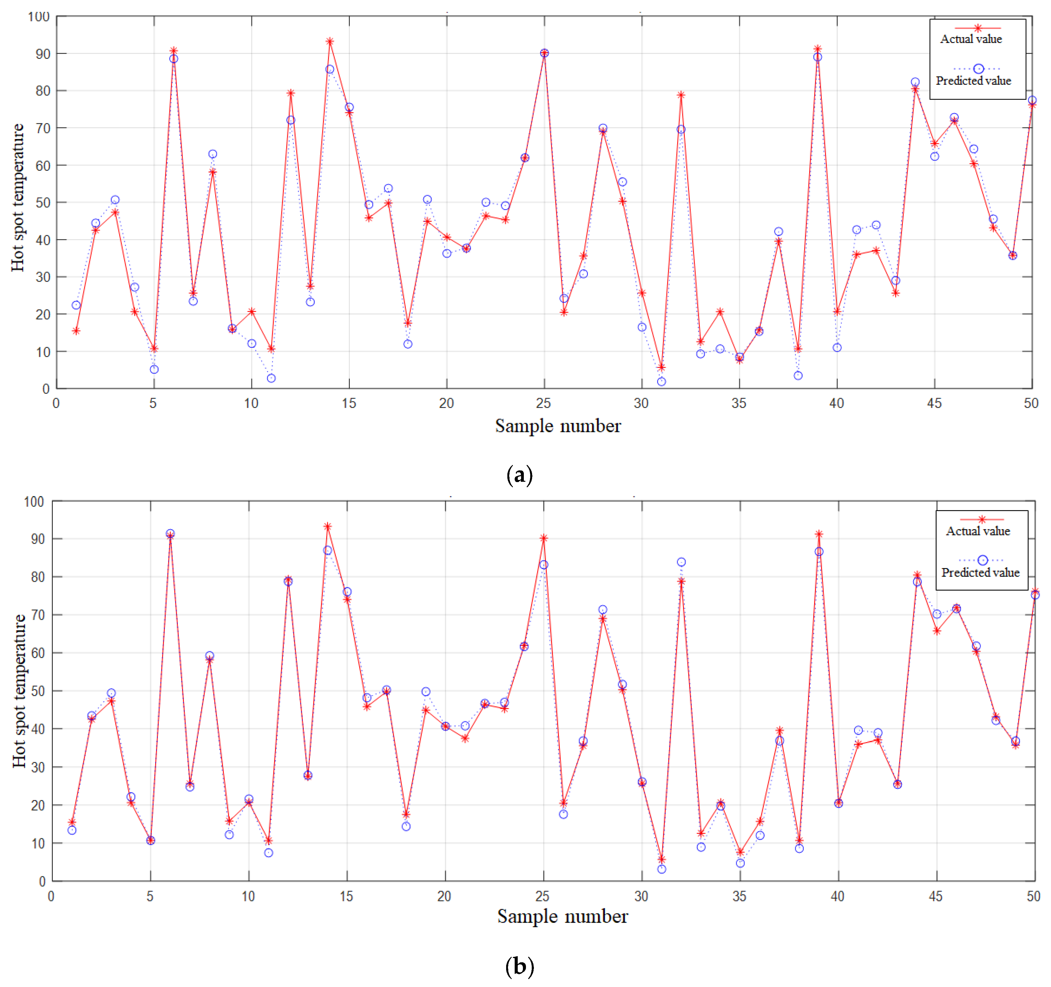
According to the results in Figure 10 and Table 3,when the ELM model is established with the skin temperature of measurement points 1 and 3, the error is 24.71; when the cascade inversion model proposed in this paper is used, the error is 6.95, which is about 3.56 times lower, and the effect is better than the direct inversion of the hotspot temperature of the middle joint.
5. Conclusions
To ensure the safe and stable functioning of power cables, it is essential to accurately calculate the temperature at the intermediate joint locations of these cables. Our research focuses on 110 kV single-core cable joints, leveraging both axial and radial heat flow dynamics to develop a sophisticated hotspot temperature cascade inversion model. The findings from this study are presented in detail below:
(1) A refined temperature field simulation model was developed using a simplified heat flow-equivalent structure approach. This model incorporates finite element techniques to simulate the steady-state temperature field effectively. By meticulously mapping hotspot temperatures and strategic skin temperature measurement points, we created a comprehensive dataset. Utilizing the neighborhood component analysis (NCA), we carefully calculated the significance of each temperature measurement point. This analysis assisted in pinpointing the most effective skin temperature measurement points, enhancing the accuracy of our temperature assessment framework;
(2) The study introduces a cascade inversion model that utilizes the extreme learning machine (ELM) algorithm to construct detailed radial and axial inversion sub-models. By modifying various model parameters, including those influencing the selection and evaluation criteria of training and test sets, substantial improvements in modeling accuracy and reliability were achieved. The training of the radial and axial inversion sub-models using selected samples from the training set significantly refined the model’s predictive capability. The overall effectiveness of the cascade inversion model was confirmed by evaluating its performance using metrics such as the mean square error (MSE) and the coefficient of determination (R2). These metrics, calculated using both core temperature data and intermediate joint hotspot temperatures from the test set samples, show that the model not only fits well with the observed data but also accurately predicts joint temperatures;
(3) A comparative analysis between the proposed cascade inversion method and a direct inversion method based solely on skin temperature measurements underscores the superiority of our approach. Firstly, the radial inversion errors of model 1 and model 2 are controlled within a small range, providing greater fault tolerance for subsequent axial inversion. The NCA algorithm significantly improves the robustness of the axial inversion model by screening skin temperature measurement points, preventing the errors generated by radial inversion from being significantly amplified. This makes the cascade inversion model achieve significantly lower mean square errors, specifically decreasing from 24.71 in the direct method to 6.95 in the cascade model. This improvement highlights the cascade model’s capacity to enhance the accuracy and reliability of hotspot temperature predictions substantially.
The thorough investigation and application of both extreme machine learning algorithms and finite element methods in this study point to the potential for significant advancements in predictive monitoring and maintenance of power cable systems. This study not only verifies the enhanced predictive accuracy of the cascade inversion model but also sets a foundation for future research in this critical field of electrical engineering.
Author Contributions
Conceptualization, X.L. and B.F.; methodology, X.L. and B.F.; software, Z.W. and J.R.; validation, C.X.; writing—original draft preparation, X.L., B.F., Z.W., J.R. and C.X. All authors have read and agreed to the published version of the manuscript.
Funding
This research was funded by National Natural Science Foundation of China (No. U2066217) and Science and Technology Project of China Southern Power Grid Company Limited (No. GDKJXM20220135).
Data Availability Statement
The data presented in this study are available on request from the corresponding author.
Conflicts of Interest
Authors Xinhai Li, Bao Feng, Zhengang Wang were employed by the company Guangdong Zhongshan Power Supply Bureau of China Southern Power Grid Co., Ltd. The remaining authors declare that the research was conducted in the absence of any commercial or financial relationships that could be construed as a potential conflict of interest.
Abbreviations
The nomenclature list for all the acronyms and parameters.
| ELM | Extreme learning machine |
| NCA | Neighbor component analysis |
| R2 | Goodness of fit |
| Se | Sensitivity coefficient |
| MSE | Mean squared error |
References
- Liu, C.; Ruan, J.; Huang, D.; Zhan, Q.; Xiao, W.; Tang, K. Hot Spot Temperature of Cable Joint Considering Contact Resistance. High Volt. Eng. 2016, 42, 3634–3640. [Google Scholar] [CrossRef]
- Wang, Y.; Li, Z.; Yang, P.; Liu, W. Calculation of Conductor Temperature and Ampacity of Directly Buried Cable Based on Electromagnetic Thermal Multi Field Coupling. Acta Metrol. Sin. 2022, 43, 877–884. [Google Scholar]
- IEC 60853: 2008; Calculation of the Cycle and Emergency Current Rating of Cables. IEC: Geneva, Switzerland, 2008.
- Liang, Y.; Wang, J. Transient Temperature Rise Calculation of Buried Power Cable Based on Thermal Circuit Model and Transient Adjoint Model. High Volt. Eng. 2022, 48, 3517–3525. [Google Scholar] [CrossRef]
- Gao, Y.; Tan, T.; Ruan, J.; Gao, J.; Liu, K. Research on Temperature Retrieval and Fault Diagnosis of Cable Joint. High Volt. Eng. 2016, 42, 535–542. [Google Scholar]
- Bates, C.; Malmedal, K.; Cain, D. Cable ampacity calculations: A comparison of methods. IEEE Trans. Indus-Try Appl. 2016, 52, 112–118. [Google Scholar] [CrossRef]
- Tang, K.; Wen, W.; Ruan, J.; Zhan, Q.; Xiao, W.; Tang, K. Temperature field simulation of single core cable based on FEM. Eng. J. Wuhan Univ. (Eng. Ed.) 2018, 51, 811–816. [Google Scholar] [CrossRef]
- Pu, L.; Duan, W.; Sun, J.; Zhao, X.; Xiong, L. Core Temperature Calculation of Single-Core Cable Joints Based on FEM. Power Syst. Clean Energy 2021, 37, 57–63. [Google Scholar]
- Zhao, X.; Hao, Y.; Huang, G.; Duan, W.; Sun, H.; Li, J.; Chen, X.; Deng, J. Calculation on Steady-state Current Carrying Capacity of Intermediate Joint of Direct Buried Cable Based on the Finite Element Simulation. High Volt. Eng. 2022, 58, 64–70+85. [Google Scholar] [CrossRef]
- IEC 60853; Calculation of the Cyclic and Emergency Current Rating of Cable—Part 2: Cyclic Rating of Cables Greater Than 18/30(36) kV and Emergency Ratings of Cables of All Voltages. IEC: Geneva, Switzerland, 1989.
- Zeng, T.; Guo, Y.; Chen, Y.; Wu, Z.; Chen, Y.; Liu, G. Effect of Filling Materials and Pipe Diameter on Cable Conductor Temperature in Pipe-laying Lines. Guangdong Electr. Power 2022, 35, 130–137. [Google Scholar]
- Lin, Z.; Zhou, H.; Niu, L.; Fu, X.; Liu, Y.; Sun, Q. Thermal-fluid coupling analysis of ultra-high voltage cables laid in tunnel. Electr. Power Eng. Technol. 2022, 41, 216–223. [Google Scholar]
- Zhang, Y.; Guo, Z.; Wang, Z.; Huang, X. Calculation and Experimental Verification of Cable Support’s Temperature Rise Based on Electromagnetic-fluid-thermal Fields. High Volt. Appar. 2019, 55, 143–148+156. [Google Scholar] [CrossRef]
- Liu, G.; Wang, P.; Mao, J.; Liu, L.; Liu, Y. Simulation Calculation of Temperature Field Distribution in High Voltage Cable Joints. High Volt. Eng. 2018, 44, 3688–3698. [Google Scholar] [CrossRef]
- Lin, Y.; Hu, Y.; Li, Q.; Zhang, A. Analysis of submarine cable temperature field and ampacity model in complex environment. J. Electron. Meas. Instrum. 2021, 35, 39–46. [Google Scholar] [CrossRef]
- Cui, R.; Xiao, P.; Wu, G.; Li, J.; Du, Z.; Hao, Z. Study on Current-carrying Improvement of J-tubes Section of ±250 kV DC Submarine Cable. High Volt. Appar. 2022, 58, 61–69. [Google Scholar] [CrossRef]
- Tang, K.; Ruan, J.; Tang, L.; Zhan, Q.; Liu, Y. Temperature Field Calculation of Three Core Cable Joint. High Volt. Eng. 2019, 45, 3571–3578. [Google Scholar]
- Jiang, Y.; Fang, Y.; Zhao, W.; Yang, Y.; Liu, X.; Li, X. Research on defect detection method of power cable based on inverse problem of temperature field. Adv. Technol. Electr. Eng. Energy 2022, 41, 81–88. [Google Scholar]
- Qin, C.; Li, B.; Li, G.; Yang, X.; Li, C. Numerical Calculation of Temperature Field of 220 kV Three-Core Submarine Cable Based on Finite Element Method. J. Northeast. Electr. Power Univ. 2019, 39, 5–10. [Google Scholar] [CrossRef]
- Chen, X.; Wang, Q.; Yu, J.; Yao, G. Simulation Research on DC Ampacity of 10 kV AC XLPE Cable under Different DC Operation Topologies and Laying Modes. High Volt. 2021, 47, 4044–4054. [Google Scholar]
- Wang, Q.; Wang, G.; Chen, X.; Yu, J. Thermo-electric Coupling Simulation Analysis for 10 kV AC XLPE Cable Changed to Tripole DC Operation under Different Laying Modes. Electr. Eng. 2022, 57, 46–54. [Google Scholar] [CrossRef]
- Niu, H.; Zheng, W.; Lei, C.; Ye, K.; Wang, Y.; Lu, G. Estimation Method for Thermal Parameters of Soil Around the Cable Based on Finite Element and Particle Swarm Optimization. High Volt. Eng. 2018, 44, 1557–1563. [Google Scholar] [CrossRef]
- Jiang, T.; Cheng, S.; Bi, M.; Chen, X.; Liu, X.; Zhang, B. Electrical-Thermal Simulation of Typical Insulation Defects in Cable Joints Based on ANSYS. J. Chongqing Univ. Technol. (Nat. Sci.) 2019, 33, 151–158. [Google Scholar]
- Zhao, L.; Zhou, D.; Wang, Z. DC transformation of 10 kV three core AC cable under different laying conditions. Electr. Power Eng. Technol. 2022, 41, 143–149. [Google Scholar]
- Zhao, L.; Zhou, D.; Yan, Z.; Li, H.; Ren, J.; Wang, Z. Study on the Thermal-Electric Couple Simulation of DC Transformation for 10 kV AC Three-Core Cable Joint. South. Power Syst. Technol. 2021, 15, 105–112. [Google Scholar] [CrossRef]
- Hao, Y.; Li, J.; Chen, X.; Deng, J.; Zhao, X.; Duan, W. Calculation of Steady-State Current Carrying Capacity of Intermediate Joint of Direct Buried DC Cable. Wire Cable 2020, 63, 30–34. [Google Scholar] [CrossRef]
Figure 1.
Diagram of the actual connector of the single-core cable. (a) Schematic diagram of the overall structure of the intermediate connector. (b) Cross-sectional structure of single-core cable body.
Figure 1.
Diagram of the actual connector of the single-core cable. (a) Schematic diagram of the overall structure of the intermediate connector. (b) Cross-sectional structure of single-core cable body.

Figure 2.
The 110 kV cable joint structure drawing.

Figure 3.
Schematic diagram of heat source loading.
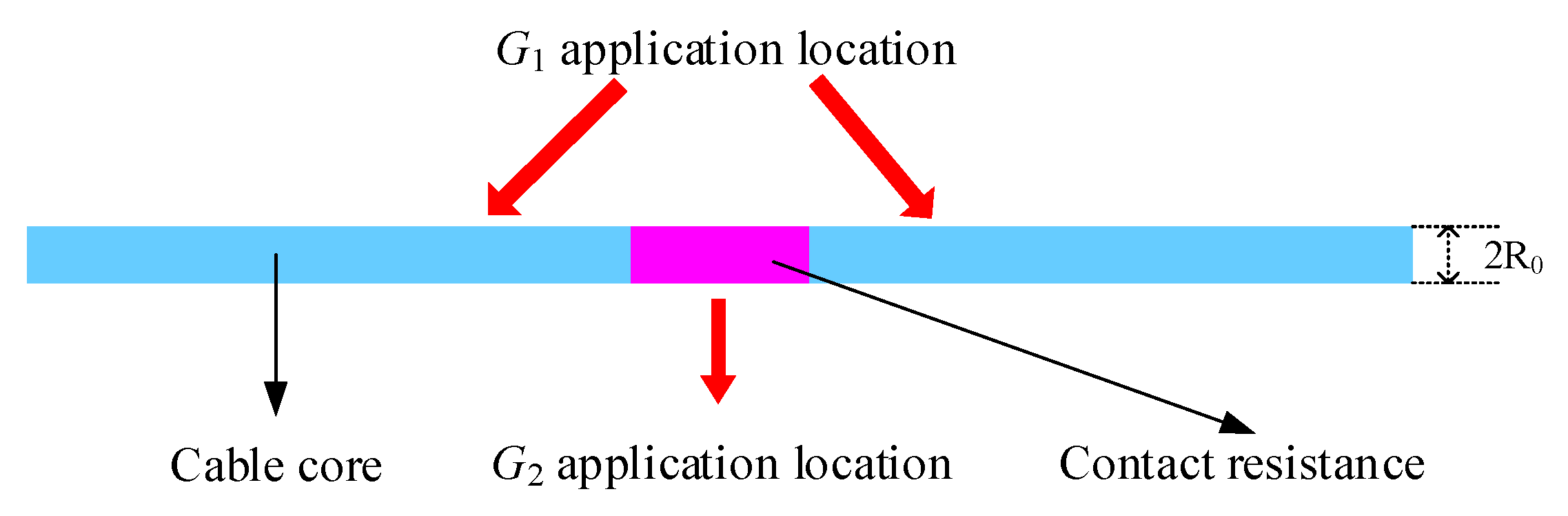
Figure 4.
The specific implementation steps of the ELM algorithm.

Figure 5.
Cascade inversion model structure.

Figure 6.
Cascade inversion model implementation process.

Figure 7.
Temperature measurement point distribution of single-core cable skin. (a) Distribution of the location of the skin temperature measurement points at the A end of the body. (b) Distribution of the location of the skin temperature measurement points at the B end of the body.
Figure 7.
Temperature measurement point distribution of single-core cable skin. (a) Distribution of the location of the skin temperature measurement points at the A end of the body. (b) Distribution of the location of the skin temperature measurement points at the B end of the body.
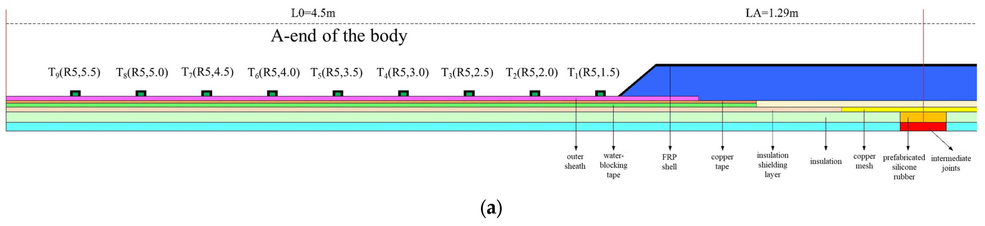

Figure 8.
NCA measurement point location selection results.
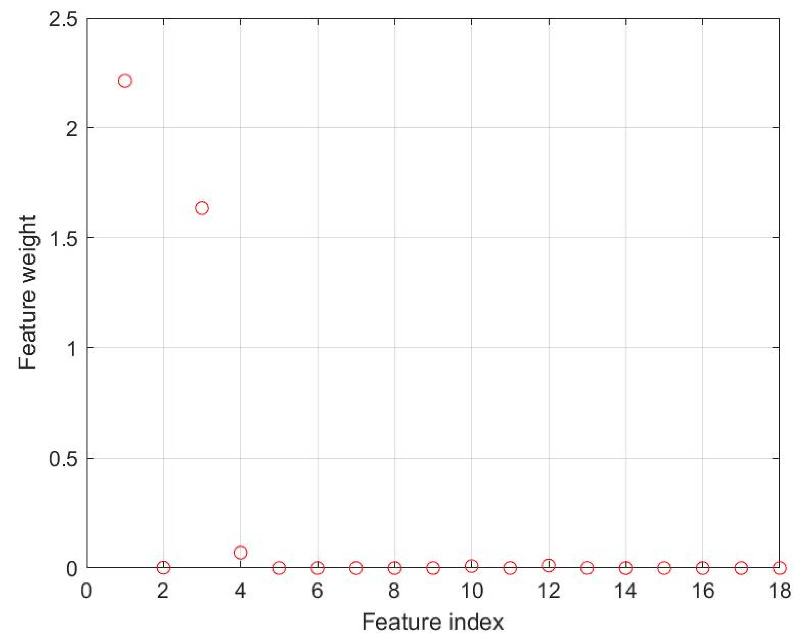
Figure 9.
Training effect of the first-level model and the second-level model. (a) Radial inversion model 1 prediction error. (b) Radial inversion model 2 prediction error. (c) Axial inversion model prediction errors.
Figure 9.
Training effect of the first-level model and the second-level model. (a) Radial inversion model 1 prediction error. (b) Radial inversion model 2 prediction error. (c) Axial inversion model prediction errors.


Figure 10.
Comparison of direct inversion and cascade inversion results. (a) Direct inversion modeling results. (b) Cascade inversion modeling results.
Figure 10.
Comparison of direct inversion and cascade inversion results. (a) Direct inversion modeling results. (b) Cascade inversion modeling results.

Table 1.
Material parameter of cable body and joint.
| Material | Structure | Density/ (kg/m3) | Thermal Conductivity/ (W/m·K) |
|---|---|---|---|
| Copper | Conductor, insulation shield, copper tape, copper mesh, contact resistance | 8900 | 401 |
| Cross-linked polyethylene | Insulation | 920 | 0.4 |
| Semi-conducting water tape | Water barrier | 1150 | 0.23 |
| Polyethylene | Outer sheath | 920 | 0.3 |
| Prefabricated silicone rubber | Joint insulation | 1100 | 0.27 |
| Fiberglass-reinforced plastic | Fiberglass-reinforced plastic shell | 1850 | 0.4 |
| Polyurethane waterproof adhesive | Sealant | 1200 | 0.357 |
Table 2.
Training model error index of the first-level model and the second-level model.
| Models | MSE | R2 |
|---|---|---|
| Radial Inversion Model 1 | 0.22933 | 0.99872 |
| Radial Inversion Model 2 | 0.42671 | 0.9974 |
| Axial Inversion Model | 4.7898 | 0.99319 |
Table 3.
Direct inversion versus cascade inversion error comparison.
| Methodology | MSE | R2 |
|---|---|---|
| Direct Inversion | 0.22933 | 0.99872 |
| Cascade inversion | 6.9502 | 0.98963 |
Disclaimer/Publisher’s Note: The statements, opinions and data contained in all publications are solely those of the individual author(s) and contributor(s) and not of MDPI and/or the editor(s). MDPI and/or the editor(s) disclaim responsibility for any injury to people or property resulting from any ideas, methods, instructions or products referred to in the content. |
© 2024 by the authors. Licensee MDPI, Basel, Switzerland. This article is an open access article distributed under the terms and conditions of the Creative Commons Attribution (CC BY) license (https://creativecommons.org/licenses/by/4.0/).
Share and Cite
MDPI and ACS Style
Li, X.; Feng, B.; Wang, Z.; Ruan, J.; Xiao, C. Study on Temperature Cascade ELM Inversion Method for 110 kV Single-Core Cable Intermediate Joints. Processes 2024, 12, 966. https://doi.org/10.3390/pr12050966
AMA Style
Li X, Feng B, Wang Z, Ruan J, Xiao C. Study on Temperature Cascade ELM Inversion Method for 110 kV Single-Core Cable Intermediate Joints. Processes. 2024; 12(5):966. https://doi.org/10.3390/pr12050966
Chicago/Turabian StyleLi, Xinhai, Bao Feng, Zhengang Wang, Jiangjun Ruan, and Chang Xiao. 2024. "Study on Temperature Cascade ELM Inversion Method for 110 kV Single-Core Cable Intermediate Joints" Processes 12, no. 5: 966. https://doi.org/10.3390/pr12050966
Note that from the first issue of 2016, this journal uses article numbers instead of page numbers. See further details here.