Spacetime Foam: From Entropy and Holography to Infinite Statistics and Nonlocality

Abstract

Due to quantum fluctuations, spacetime is foamy on small scales. The degree of foaminess is found to be consistent with holography, a principle prefigured in the physics of black hole entropy. It has bearing on the ultimate accuracies of clocks and measurements and the physics of quantum computation. Consistent with existing archived data on active galactic nuclei from the Hubble Space Telescope, the application of the holographic spacetime foam model to cosmology requires the existence of dark energy which, we argue, is composed of an enormous number of inert “particles” of extremely long wavelength. We suggest that these “particles” obey infinite statistics in which all representations of the particle permutation group can occur, and that the nonlocality present in systems obeying infinite statistics may be related to the nonlocality present in holographic theories. We also propose to detect spacetime foam by looking for halos in the images of distant quasars, and argue that it does not modify the GZK cutoff in the ultra-high energy cosmic ray spectrum and its contributions to time-of-flight differences of high energy gamma rays from distant GRB are too small to be detectable.

There is no excellent beauty that hath not some strangeness in the proportion.

— Francis Bacon

1. Introduction

Following John Wheeler, many physicists (including the author) believe that space is composed of an ever-changing arrangement of bubbles called spacetime foam, also known as quantum foam. To understand the terminology, let us consider the following simplified analogy which Wheeler gave in a conference on gravity at University of North Carolina in 1957. Imagine yourself flying an airplane over an ocean. At high altitude the ocean appears smooth. But as you descend, it begins to show roughness. Close enough to the ocean surface, you see bubbles and foam. Analogously, spacetime appears smooth on a large scale, but on sufficiently small scales, it will appear rough and foamy, hence the term “spacetime foam” [1]. Many physicists believe the foaminess is due to quantum fluctuations of spacetime, hence the alternative term “quantum foam.” This reveiw article is devoted to a discussion of spacetime foam models, or rather, a specific one of them for which the concept of entropy plays a crucial role [2,3,4,5,6]. The only ingredients we use in the whole discussion are quantum mechanics and general relativity, the two pillars of modern physics. We hope that the results are very general and have wider validity than most of the candidates of quantum gravity theory. Assuming that there is a unity of physics connecting the Planck scale to the cosmic scale, we also apply quantum foam physics to cosmology [7,8,9].

In the next section, by a process of mapping the geometry of a region of spacetime, we show how foamy spacetime is. It turns out that the degree of foaminess of spacetime determines the maximum amount of entropy a spatial region can hold. This maximum amount of information can be shown to be consistent with that encoded in the holographic principle which has its origin in black hole physics. Appropriately this spacetime foam model has come to be known as the holographic model. In section 3, we propose to probe spacetime foam by looking for halos in the images of distant quasars or bright active galactic nuclei (AGN). There we show that the archive from the Hubble Space Telescople (HST) can already be used to yield useful bounds. Among the spacetime foam models, the holographic foam model is unique in its correspondence with the case of maximum energy density that a spatial region can hold without collapsing into a black hole. Applied to cosmology it “predicts” a critical energy density as observed in recent years. This potential connection between the extremely large and the extremely small is explored in section 4; there we show that the archive on quasars and AGN from HST can be used, in conjuction with the physics of quantum computation, to “prove” the existence of dark energy, independent of the various cosmological observations of recent years. Indeed, from our perspective, dark energy is arguably a cosmological manifestation of quantum foam! In section 5, we examine how and why dark energy is so different from ordinary energy/matter. There we show that the holographic model of spacetime foam naturally leads us to speculate that dark energy consists of an incredibly large number of extremely-long-wavelength “particles”. Then we exploit the positivity of the entropy for these particles to show that they obey not the ordinary bose or fermi statistics, but the exotic infinite statistics (also known as quantum Boltzmann statistics). We start our discussion with holography and end with infinite statistics. We conclude section 5 by speculating that the nonlocality known to be present in both of them may be related to each other. We give a summary in section 6.

For completeness, we discuss various other relevant topics of spacetime foam physics in six short appendices. In Appendix A, using a gedanken experiment to measure distances we rederive the holographic foam model. In Appendix B, we apply the results in Appendix A to set bounds on the accuracies of clocks and limits on computations, and derive the black hole entropy and lifetime. We derive the holographic principle and the Margolus-Levitin theorem (which is liberally used in the text) in Appendix C and Appendix D respectively. Appendix E is devoted to a discussion of the uncertainties in energy-momentum measurements consistent with spacetime foam. In Appendix F we apply the results obtained in Appendix E to discuss high-energy γ rays from distant gamma ray bursts and ultra-high energy cosmic ray events.

On notations, the subscript “P” denotes Planck units; thus $l_P\equiv {(\hslash G/c^3)}^{1/2}\sim {10}^{-33}$ cm is the Planck length etc. On units, $k_B$ (the Boltzmann constant) and sometimes ℏ and c are put equal to 1 for simplicity.

A note is in order: we are well aware of some critical papers that present a viewpoint that is contrary to some of the ideas contained in this paper. See, e.g., [10] and references contained therein.

2. Quantum Fluctuations of Spacetime

2.1. Mapping the Geometry of Spacetime

If spacetime indeed undergoes quantum fluctuations, the fluctuations will show up when we measure a distance l, in the form of uncertainties in the measurement. The question now is: how accurately can we measure this distance? Let us denote by $\delta l$ the accuracy with which we can measure l. We will also refer to $\delta l$ as the uncertainty or fluctuation of the distance l for reasons that will become obvious shortly. One way to find $\delta l$ is to carry out a gedanken experiment to measure l. This is done in Appendix A. But, for later use, it is more convenient to find $\delta l$ by carrying out a process of mapping the geometry of spacetime. This method [6,11] relies on the fact that quantum fluctuations of spacetime manifest themselves in the form of uncertainties in the geometry of spacetime. Hence the structure of spacetime foam can be inferred from the accuracy with which we can measure that geometry. Let us consider mapping out the geometry of spacetime for a spherical volume of radius l over the amount of time $T=2l/c$ it takes light to cross the volume. One way to do this is to fill the space with clocks, exchanging signals with other clocks and measuring the signals’ times of arrival. This process of mapping the geometry of spacetime is a kind of computation, in which distances are gauged by transmitting and processing information. The total number of operations, including the ticks of the clocks and the measurements of signals, is bounded by the Margolus-Levitin theorem [12](see Appendix D) in quantum computation, which stipulates that the rate of operations for any computer cannot exceed the amount of energy E that is available for computation divided by $\pi \hslash /2$. A total mass M of clocks then yields, via the Margolus-Levitin theorem, the bound on the total number of operations given by $(2M{c}^2/\pi \hslash )\times 2l/c$. But to prevent black hole formation, M must be less than $l{c}^2/2G$. Together, these two limits imply that the total number of operations that can occur in a spatial volume of radius l for a time period $2l/c$ is no greater than $2{(l/l_P)}^2/\pi$. To maximize spatial resolution, each clock must tick only once during the entire time period. The operations can be regarded as partitioning the spacetime volume into "cells", then on the average each cell occupies a spatial volume no less than $(4\pi l^3/3)/(2l^2/\pi l_P^2)=2{\pi }^{2}l{l}_P^2/3$, yielding an average separation between neighhoring cells no less than ${(2{\pi }^2/3)}^{1/3}{l}^{1/3}{l}_P^{2/3}$. This spatial separation is interpreted as the average minimum uncertainty [13] in the measurement of a distance l, that is,

$$\delta l\gtrsim l^{1/3}{l}_P^{2/3},$$

(1)

where and henceforth (with a couple of exceptions) we drop multiplicative factors of order 1.

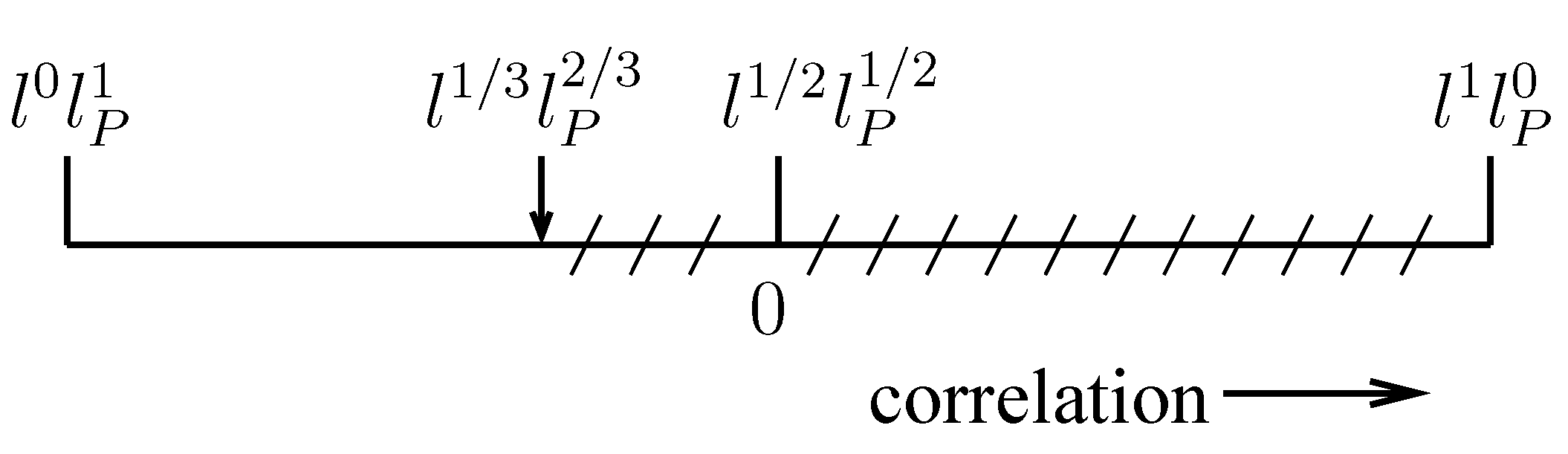
2.2. Models of Spacetime Foam

We can now understand why this quantum foam model has come to be known as the holographic model. Since, on the average, each cell occupies a spatial volume of $l{l}_P^2$, a spatial region of size l can contain no more than $l^3/\left(l{l}_P^2\right)={(l/l_P)}^2$ cells. Thus this model corresponds to the case of maximum number of bits of information $l^2/l_P^2$ in a spatial region of size l, that is allowed by the holographic principle [14] (see AppendixC).

To see this more concretely, consider a cubic region of space with linear dimension l. Conventional wisdom claims that the region can be partitioned into cubes as small as ${\left(l_P\right)}^3$. It follows that the number of degrees of freedom of the region is bounded by ${(l/l_P)}^3$, i.e., the volume of the region in Planck units. But conventional wisdom is wrong, for according to Eq. (1), the smallest cubes into which we can partition the region cannot have a linear dimension smaller than ${\left(l{l}_P^2\right)}^{1/3}$. Therefore, the number of degrees of freedom of the region is bounded by ${[l/{\left(l{l}_P^2\right)}^{1/3}]}^3$, i.e., the area of the region in Planck units, as stipulated by the holographic principle [14].

Recently Gambini and Pullin [15] have shown that holography follows from the framework of loop quantum gravity in spherical symmetry. They have derived from first principles an uncertainty in the determination of volumes that grows radially (corresponding to the l above); i.e., they have recovered Eq. (1).

It will prove to be useful to compare the holographic model in the mapping of the geometry of spacetime with the one that corresponds to spreading the spacetime cells uniformly in both space and time. For the latter case, each cell has the size of ${\left(l^2{l}_P^2\right)}^{1/4}=l^{1/2}{l}_P^{1/2}$ both spatially and temporally so that each clock ticks once in the time it takes to communicate with a neighboring clock. Since the dependence on $l^{1/2}$ is the hallmark of a random-walk fluctuation, this quantum foam model corresponding to $\delta l\gtrsim {\left(l{l}_P\right)}^{1/2}$ is called the random-walk model [16]. Compared to the holographic model, the random-walk model predicts a coarser spatial resolution, i.e., a larger distance fluctuation, in the mapping of spacetime geometry. It also yields a smaller bound on the information content in a spatial region, viz., ${(l/l_p)}^2/{(l/l_P)}^{1/2}={(l^2/l_P^2)}^{3/4}={(l/l_P)}^{3/2}$ bits.

Actually there are many other models of spacetime foam, in addition to the holographic model and the random-walk model. We can parametrize them according to $\delta l\sim l^{1-\alpha }{l}_P^{\alpha }$ for α of order 1, with $\alpha =2/3$ and $1/2$ for the holographic model and the random-walk model respectively [17].

Note that the minimum $\delta l$ just found for the holographic model corresponds to the case of maximum energy density $\rho =(3/8\pi ){\left(l{l}_P\right)}^{-2}$ for a sphere of radius l not to collapse into a black hole. Hence the holographic model, unlike the other models, requires, for its consistency, the energy density to have the critical value. By contrast, for instance, the random-walk model corresponds to an energy density ${\left(l{l}_P\right)}^{-2}\gtrsim \rho \gtrsim l^{-5/2}{l}_P^{-3/2}$. (The upper bound corresponds to the clocks ticking every ${\left(l{l}_P\right)}^{1/2}$ while the lower bound corresponds to the clocks ticking only once during the entire time $2l/c$.)

2.3. Cumulative Effects of Spacetime Fluctuations

Let us examine the cumulative effects [18] of spacetime fluctuations over a large distance. Consider a distance l, and divide it into $l/\lambda$ equal parts each of which has length λ (that can be as small as $l_P$). If we start with $\delta \lambda$ from each part, the question is how do the $l/\lambda$ parts add up to $\delta l$ for the whole distance l. In other words, we want to find the cumulative factor C defined by $\delta l=C\delta \lambda$. Since $\delta l\sim l^{1/3}{l}_P^{2/3}=l_P{(l/l_P)}^{1/3}$ and $\delta \lambda \sim {\lambda }^{1/3}{l}_P^{2/3}=l_P{(\lambda /l_P)}^{1/3}$, the result is $C={(l/\lambda )}^{1/3}$. Note that the cumulative factor is not linear in $(l/\lambda )$, i.e., $\frac{\delta l}{\delta \lambda }\ne \frac{l}{\lambda }$. (In general, it is much smaller than $l/\lambda$). The reason for this is obvious: the $\delta \lambda$’s (which take on ± sign with equal probability) from the $l/\lambda$ parts in l do not add coherently. In general, for spacetime foam models corresponding to $\delta l\sim l^{1-\alpha }{l}_P^{\alpha }$, the cumulative factor is given by $C={(l/\lambda )}^{1-\alpha }$. Thus for the random-walk model, the cumulative factor is ${(l/\lambda )}^{1/2}$. Note that for the holographic case, the individual fluctuations cannot be completely random (as opposed to the random-walk model); strangely successive fluctuations appear to be entangled and somewhat anti-correlated (i.e., a plus fluctuation is slightly more likely followed by a minus fluctuation and vice versa), in order that together they produce a total fluctuation less than that in the random-walk model. This small amount of anti-correlation between successive fluctuations (corresponding to what statisticians call fractional Brownian motion with self-similarity parameter $\frac{1}{3}$) must be due to quantum gravity effects.

On the other hand, if successive fluctuations are completely anti-correlated, then the fluctuation of a distance l is given by the minuscule $l_P$, independent of the size of the distance. For completeness, we mention that a priori there are also models with positive correlations between successive fluctuations. But these models yield unacceptably large fluctuations in distance measurements — it turns out (see next section) that these models (actually all models with $\alpha \lesssim 0.6$ corresponding to the hatched line in Fig. 1) have already been observationally ruled out.

Figure 1. Lower bounds on $\delta l$ for the various quantum gravity models. The fluctuation of a distance l is given by the sum of $l/l_P$ fluctuations each by plus or minus $l_P$. Spacetime foam appears to choose a small anti-correlation (i.e., negative correlation) between successive fluctuations, giving a cube root dependence in the number $l/l_p$ of fluctuations for the total fluctuation of l (indicated by the arrow). The corresponding model falls between the two extreme cases of complete randomness, i.e., zero correlation (corresponding to $\delta l\sim l^{1/2}{l}_P^{1/2}$) and complete anti-correlation (corresponding to $\delta l\sim l_P$).

Figure 1. Lower bounds on $\delta l$ for the various quantum gravity models. The fluctuation of a distance l is given by the sum of $l/l_P$ fluctuations each by plus or minus $l_P$. Spacetime foam appears to choose a small anti-correlation (i.e., negative correlation) between successive fluctuations, giving a cube root dependence in the number $l/l_p$ of fluctuations for the total fluctuation of l (indicated by the arrow). The corresponding model falls between the two extreme cases of complete randomness, i.e., zero correlation (corresponding to $\delta l\sim l^{1/2}{l}_P^{1/2}$) and complete anti-correlation (corresponding to $\delta l\sim l_P$).

3. Probing Quantum Foam with Extragalactic Sources

The Planck length $l_P\sim {10}^{-33}$ cm is so short that we need an astronomical (even cosmological) distance l for its fluctuation $\delta l$ to be detectable. Let us consider light (with wavelength λ) from distant quasars or bright active galactic nuclei [18,19]. Due to the quantum fluctuations of spacetime, the wavefront, while planar, is itself “foamy”, having random fluctuations in phase [18] $\Delta \varphi \sim 2\pi \delta l/\lambda$ and in the direction of the wave vector [7] given by $\Delta \varphi /2\pi$ (for $\delta l\ll \lambda$). In effect, spacetime foam creates a “seeing disk” whose angular diameter is $\sim \Delta \varphi /2\pi$. For an interferometer with baseline length D, this means that dispersion will be seen as a spread in the angular size of a distant point source, causing a reduction in the fringe visibility when $\Delta \varphi /2\pi \sim \lambda /D$. For a quasar of 1 Gpc away, at infrared wavelength, the holographic model predicts a phase fluctuation $\Delta \varphi \sim 2\pi \times {10}^{-9}$ radians. On the other hand, an infrared interferometer (like the Very Large Telescope Interferometer) with $D\sim 100$ meters has $\lambda /D\sim 5\times {10}^{-9}$. Thus, in principle, this method will allow the use of interferometry fringe patterns to test the holographic model! Furthermore, these tests can be carried out without guaranteed time using archived high resolution, deep imaging data on quasars, and possibly, supernovae from existing and upcoming telescopes.

The key issue here is the sensitivity of the interferometer. The lack of observed fringes may simply be due to the lack of sufficient flux (or even just effects originated from the turbulence of the Earth’s atmosphere) rather than the possibility that the instrument has resolved a spacetime foam generated halo. But, given sufficient sensitivity, the VLTI, for example, with its maximum baseline, presumably has sufficient resolution to detect spacetime foam halos for low redshift quasars, and in principle, it can be even more effective for the higher redshift quasars. Note that the test is simply a question of the detection or non-detection of fringes. It is not a question of mapping the structure of the predicted halo.

In the meantime, we can use existing archived data on quasars or active galactic nuclei from the Hubble Space Telescope to test the quantum foam models [7]. Consider the case of PKS1413+135 [20], an AGN for which the redshift is $z=0.2467$. With $l\approx 1.2$ Gpc and $\lambda =1.6\mu$m, we [18] find $\Delta \varphi \sim 10\times 2\pi$ and ${10}^{-9}\times 2\pi$ for the random-walk model and the holographic model of spacetime foam respectively. With $D=2.4$ m for HST, we expect to detect halos if $\Delta \varphi \sim {10}^{-6}\times 2\pi$. Thus, the HST image only fails to test the holographic model by 3 orders of magnitude.

However, the absence of a quantum foam induced halo structure in the HST image of PKS1413+135 rules out convincingly the random-walk model. (In fact, the scaling relation discussed above indicates that all spacetime foam models with $\alpha \lesssim 0.6$ are ruled out by this HST observation.) As we will see in the next section, this result has profound implications for cosmology [6,7,8,9].

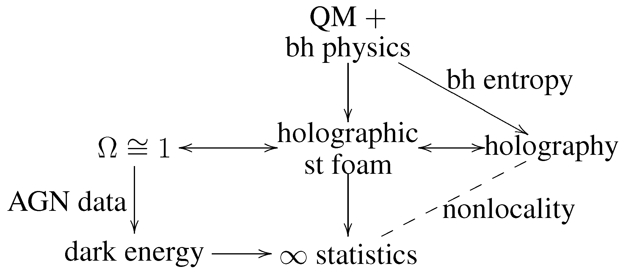
4. From Quantum Foam to (Holographic Foam) Cosmology

We can draw a useful conclusion [6,7,8,9] from the observed cosmic critical density in the present era (consistent with the prediction of the cosmology based on the holographic model of spacetime foam, which henceforth we call the holographic foam cosmology (HFC)) $\rho \sim H_0^2/G\sim {\left(R_H{l}_P\right)}^{-2}$ (about ${10}^{-9}$ joule per cubic meter), where $H_0$ is the present Hubble parameter of the observable universe and $R_H$ is the Hubble radius. Treating the whole universe as a computer[6,21], one can apply the Margolus-Levitin theorem to conclude that the universe computes at a rate ν up to $\rho R_H^3\sim R_H{l}_P^{-2}$ ($\sim {10}^{106}$ op/sec), for a total of ${(R_H/l_P)}^2$ ($\sim {10}^{122}$) operations during its lifetime so far. If all the information of this huge computer is stored in ordinary matter, then we can apply standard methods of statistical mechanics to find that the total number I of bits is ${\left[{(R_H/l_P)}^2\right]}^{3/4}={(R_H/l_P)}^{3/2}$ ($\sim {10}^{92}$). It follows that each bit flips once in the amount of time given by $I/\nu \sim {\left(R_H{l}_P\right)}^{1/2}$ ($\sim {10}^{-14}$ sec). On the other hand, the

Table 1. Random-walk model versus holographic model. The corresponding quantities for the random-walk model (second row) and the holographic model (third row) of spacetime foam (STF) appear in the same columns in the following Table. (Entropy is measured in Planck units.)

STF	distance	entropy	energy	matter/	type of
model	fluctuations	bound	density	energy	statistics
random-	$\delta l\gtrsim l^{1/2}{l}_P^{1/2}$	${\left(Area\right)}^{3/4}$	${\left(l{l}_P\right)}^{-2}\gtrsim \rho$	ordinary	bose /
walk			$\gtrsim l^{-5/2}{l}_P^{-3/2}$		fermi
holo-	$\delta l\gtrsim l^{1/3}{l}_P^{2/3}$	$Area$	$\rho \lesssim {\left(l{l}_P\right)}^{-2}$	dark	infinite
graphic				energy

Table 1. Random-walk model versus holographic model. The corresponding quantities for the random-walk model (second row) and the holographic model (third row) of spacetime foam (STF) appear in the same columns in the following Table. (Entropy is measured in Planck units.)

STF	distance	entropy	energy	matter/	type of
model	fluctuations	bound	density	energy	statistics
random-	$\delta l\gtrsim l^{1/2}{l}_P^{1/2}$	${\left(Area\right)}^{3/4}$	${\left(l{l}_P\right)}^{-2}\gtrsim \rho$	ordinary	bose /
walk			$\gtrsim l^{-5/2}{l}_P^{-3/2}$		fermi
holo-	$\delta l\gtrsim l^{1/3}{l}_P^{2/3}$	$Area$	$\rho \lesssim {\left(l{l}_P\right)}^{-2}$	dark	infinite
graphic				energy

average separation of neighboring bits is ${(R_H^3/I)}^{1/3}\sim {\left(R_H{l}_P\right)}^{1/2}$ ($\sim {10}^{-3}$ cm). Hence, assuming only ordinary matter exists to store all the information in the universe results in the conclusion that the time to communicate with neighboring bits is equal to the time for each bit to flip once. It follows that the accuracy to which ordinary matter maps out the geometry of spacetime corresponds exactly to the case of events spread out uniformly in space and time discussed above for the case of the random-walk model of spacetime foam.

But, as shown in the previous section, the sharp images of distant quasars or active galactic nuclei observed at the Hubble Space Telescope have ruled out the random-walk model. From the demise of the random-walk model and the fact that ordinary matter only contains an amount of information dense enough to map out spacetime at a level consistent with the random-walk model, one can now infer that spacetime must be mapped to a finer spatial accuracy than that which is possible with the use of ordinary matter. But if ordinary matter does not do, there must be another kind of substance with which spacetime can be mapped to the observed accuracy, conceivably as given by the holographic model. The natural conclusion [7,8,9] is that unconventional (dark [22]) energy/matter exists! Note that this argument does not make use of the evidence from recent cosmological (supernovae, cosmic microwave background, and galaxy clusters) observations [23].

A comparison between what the random-walk model and the holographic model yield for the entropy bound etc. is given in Table 1. See the next section for the explanation of the last column.

The fact that our universe is observed to be at or very close to its critical density must be taken as solid albeit indirect evidence in favor of the holographic model because, as discussed above, it is the only model that requires, for its consistency, the maximum energy density without causing gravitational collapse. Specifically, according to the HFC, the cosmic density is

$$\rho =(3/8\pi ){\left(R_H{l}_P\right)}^{-2}\sim {(H/l_P)}^2,$$

(2)

and the cosmic entropy is given by

$$I\sim {(R_H/l_P)}^2.$$

(3)

Thus the average energy carried by each bit is $\rho R_H^3/I\sim R_H^{-1}$ ($\sim {10}^{-31}$ eV). Such long-wavelength (hence “non-local”) bits or “particles” carry negligible kinetic energy. Also according to HFC, it takes each unconventional bit the amount of time $I/\nu \sim R_H$ to flip. Thus, on the average, each bit flips once over the course of cosmic history. Compared to the conventional bits carried by ordinary matter, these bits are rather passive and inert (which, by the way, may explain why dark energy is dark). This is understandable since each unconventional bit has, at its disposal, only such a minuscule amount of energy. But together (there can be as many as ${(R_H/l_P)}^2\sim {10}^{123}$ of them in the present observable universe, far outnumbering the ${10}^{92}$ or so particles of ordinary matter and radiation), they supply the missing mass/energy of the universe. Accelerating the cosmic expansion is a relatively simple task, computationally speaking.

5. Infinite Statistics and Nonlocality

5.1. Infinite Statistics

What is the overriding difference between conventional matter and unconventional energy/matter (i.e., dark energy and perhaps also dark matter)? To find that out, let us first consider a perfect gas of N particles obeying Boltzmann statistics (which, rigorously speaking, is not a physical statistics but is still a useful statistics to work with) at temperature T in a volume V. For the problem at hand, as the lowest-order approximation, we can neglect the contributions from matter and radiation to the cosmic energy density for the recent and present eras. Then the Friedmann equations for $\rho \sim H^2/G$ can be solved by $H\propto 1/a$ and $a\propto t$, where $a\left(t\right)$ is the cosmic scale factor. Thus let us take $V\sim R_H^3$, $T\sim R_H^{-1}$, and $N\sim {(R_H/l_P)}^2$. A standard calculation (for the relativistic case) yields the partition function $Z_N={(N!)}^{-1}{(V/{\lambda }^3)}^N$, where $\lambda ={\left(\pi \right)}^{2/3}/T$. With the free energy given by $F=-Tln{Z}_N=-NT[ln(V/N{\lambda }^3)+1]$, we get, for the entropy of the system,

$$S=-{(\partial F/\partial T)}_{V,N}=N[ln(V/N{\lambda }^3)+5/2].$$

(4)

For the non-relativistic case with the effective mass $m\sim R_H^{-1}$ (coming from some sort of potential with which we are not going to concern ourselves), the only changes in the above expressions are given by the substitution $\lambda ⟶{(2\pi /mT)}^{1/2}$. With $m\sim T\sim R_H^{-1}$, there is no significant qualitative difference between the non-relativistic and relativistic cases.

The important point to note is that, since $V\sim {\lambda }^3$, the entropy S in Eq. (4) becomes nonsensically negative unless $N\sim 1$ which is equally nonsensical because N should not be too different from ${(R_H/l_P)}^2\gg 1$. Intentionally we have calculated the entropy by employing the familiar Boltzmann statistics (with the correct Boltzmann counting factor), only to arrive at a contradictory result. But now the solution to this contradiction is pretty obvious: the N inside the log in Eq. (4) somehow must be absent. Then $S\sim N\sim {(R_H/l_P)}^2$ without N being small (of order 1) and S is non-negative as physically required. That is the case if the “particles” are distinguishable and nonidentical! For in that case, the Gibbs $1/N!$ factor is absent from the partition function $Z_N$, and the entropy becomes

$$S=N[ln(V/{\lambda }^3)+3/2].$$

(5)

Now the only known consistent statistics in greater than two space dimensions without the Gibbs factor (recall that the Fermi statistics and Bose statistics give similar results as the conventional Boltzmann statistics at high temperature) is infinite statistics (sometimes called “quantum Boltzmann statistics”) [24,25,26]. Thus we have shown that the “particles” constituting dark energy obey infinite statistics, instead of the familiar Fermi or Bose statistics [9]. What is infinite statistics? Succinctly, a Fock realization of infinite statistics is provided by a q deformation of the commutation relations of the oscillators: $a_k{a}_l^{†}-q{a}_l^{†}{a}_k={\delta }_{kl}$ with q between -1 and 1 (the case $q=\pm 1$ corresponds to bosons or fermions). States are built by acting on a vacuum which is annihilated by $a_k$. Two states obtained by acting with the N oscillators in different orders are orthogonal. It follows that the states may be in any representation of the permutation group. The statistical mechanics of particles obeying infinite statistics can be obtained in a way similar to Boltzmann statistics, with the crucial difference that the Gibbs $1/N!$ factor is absent for the former. Infinite statistics can be thought of as corresponding to the statistics of identical particles with an infinite number of internal degrees of freedom, which is equivalent to the statistics of nonidentical particles since they are distinguishable by their internal states.

5.2. Nonlocality

Infinite statistics appears to have one “defect”: a theory of particles obeying infinite statistics cannot be local [26,27,28]. (That is, the fields associated with infinite statistics are not local, neither in the sense that their observables commute at spacelike separation nor in the sense that their observables are pointlike functionals of the fields.) The expression for the number operator (for the case of $q=0$)

$$n_i=a_i^{†}{a}_i+\sum _k{a}_k^{†}{a}_i^{†}{a}_i{a}_k+\sum _l\sum _k{a}_l^{†}{a}_k^{†}{a}_i^{†}{a}_i{a}_k{a}_l+\dots ,$$

(6)

is both nonlocal and nonpolynomial in the field operators, and so is the Hamiltonian. The lack of locality may make it difficult to formulate a relativistic verion of the theory; but it appears that a non-relativistic theory can be developed. Lacking locality also means that the familiar spin-statistics relation is no longer valid for particles obeying infinite statistics; hence they can have any spin. Remarkably, the TCP theorem and cluster decomposition have been shown to hold despite the lack of locality [26].

Actually the lack of locality for theories of infinite statistics may have a silver lining. According to the holographic principle, the number of degrees of freedom in a region of space is bounded not by the volume but by the surrounding surface. This suggests that the physical degrees of freedom are not independent but, considered at the Planck scale, they must be infinitely correlated, with the result that the spacetime location of an event may lose its invariant significance. Since the holographic principle is believed to be an important ingredient in the formulation of quantum gravity, the lack of locality for theories of infinite statistics may not be a defect; it can actually be a virtue. Perhaps it is this lack of locality that makes it easier to incorporate gravitational interactions in the theory. Quantum gravity and infinite statistics appear to fit together nicely, and nonlocality seems to be a common feature of both of them [9].

We note the following related work. Using the Matrix theory approach, Jejjala, Kavic and Minic [29] have argued that dark energy quanta obey infinite statistics (and that the fine structure of dark energy is governed by a Wien distribution). They have also concluded that the non-locality present in systems obeying infinite statistics and the non-locality present in holographic theories may be related.

Strominger [30] has shown that the wave function of many similarly charged extremal black holes depends on each black hole’s position, and thus the black holes can be considered as distinguishable and accordingly obey infinite statistics.

Figure 2. Connecting the different ideas.

Figure 2. Connecting the different ideas.

More generally Giddings [31] has observed that the non-perturbative dynamics of gravity is nonlocal. His argument is based on several reasons: lack of a precise definition in quantum gravity –connected with the apparent absence of local observables; indications from high-energy gravitational scattering; hints from string theory, particularly the AdS/CFT correspondence; conundrums of quantum cosmology; and the black hole information paradox. Horowitz [32] has noted that quantum gravity may need some violation of locality; thus when one reconstructs the string theory from the gauge theory (in the AdS/CFT correspondence), physics may not be local on all length scales. Meanwhile Ahluwalia [33] has argued that when measurement processes involve energies of the order of the Planck scale, the fundamental assumption of locality may no longer be a good approximation. He has shown that position measurements alter the spacetime metric in a fundamental manner and this unavoidable change in the spacetime metric destroys the commutativity (and hence locality) of position measurement operators.

6. Summary, Discussion and Conclusion

A short summary of this review article is given by the accompanying flow chart Figure 2.

Starting from quantum mechanics and some rudimentary black hole physics (viz, there is an upper bound of matter/energy that can be put in a spatial region without the region collapsing into a black hole), we derive the holographic model of spacetime foam. From the simple observation that the cosmic energy density is critical (i.e., the density parameter of the universe $\Omega \cong 1$), aided by some archived data on quasar or AGN from the Hubble Space Telescope, we are led to conclude that dark energy exists. This observation is a solid piece of evidence in favor of the holographic foam model which, after all, “predicts” that the cosmic energy density has the critical value. One is then invited to apply the holographic model to cosmology, leading to the logical speculation that the constituents of dark energy obey infinite statistics. We have now come full circle, starting with holography and ending with infinite statistics, with both sharing one common property: nonlocality. In the whole discussion, entropy plays a leading role, first in motivating holography, and secondly in determining, via its positivity property, that the “particles” constituting dark energy obey infinite statistics.

We conclude with some observation and a partial list of open questions.

(1) We have considered a perfect gas consisting of “particles” of extremely long wavelength, obeying Boltzmann statistics in the Universe at temperature T. But we have seen that these “particles” have had interactions only of order one time on the average during the entire cosmic history. A question can be raised as to whether such an inert gas can come to thermal equilibrium at any well defined temperature. We do not have a good answer; but the fact that all these “particles”, though extremely inert, have a wavelength comparable to the observable Hubble radius may mean that they overlap significantly, and accordingly can perhaps share a common temperature.

(2) These “particles” provide a (more or less) spatially uniform energy density, like a time-dependent cosmological constant [34]. But in a way, this type of models is preferrable to the cosmological constant because it may be easier to understand a zero cosmological constant (perhaps due to a certain not-yet-understood symmetry or initial condition [35]) than an exceedingly small (but non-zero) cosmological constant.

(3) Recall that earlier cosmic epochs are associated with $\rho \propto a^{-4}$ (radiation-domination) and (followed by) $\rho \propto a^{-3}$ (matter-domination). In a scenario of the holographic foam cosmology we are pursuing, these epochs are succeeded by the dark-energy-dominated era with $\rho \propto a^{-2}$. We note that the successes of the conventional big bang cosmology, such as the primordial nucleosynthesis, are not affected by this form of dark energy.

(4) An obvious question concerns the sign of the pressure for the gas of dark energy “particles”. For cosmic energy density $\rho \sim H^2/G$ with $H\propto 1/a$, the equation of state is given by $w=p/\rho \sim -1/3$, not negative enough to give an accelerating expansion. However, it has been pointed out by Zimdahl and Pavon [36] that a transition from an earlier decelerating to a recent and present accelerating cosmic expansion can arise as a pure interaction phenomenon if pressureless dark matter is coupled to holographic dark energy with $\rho \propto H^2$ [37]. As a bonus, within the framework of such cosmological models, we can now understand why, in addition to dark energy, dark matter has to exist. On the other hand, this scenario will become less natural if the equation of state w turns out to be very close to $-1$.

(5) Critical cosmic energy density is the hallmark of the inflationary paradigm [38]. Can the holographic foam cosmology (which requires $\Omega \cong 1$) supplement inflation in solving cosmological problems and in providing the necessary primordial perturbations to yield the observed astronomical structures? What are the phenomenological consequences of HFC?

(6) While it appears quite reasonable that holography (and quantum gravity in general) and infinite statistics are compatible, exactly how they are related is not yet clear. In particular, how is the nonlocality in holography related to the nonlocality present in theories with infinite statistics? (We venture a guess: Entropy is the common link, so it may hold the key in understanding the relation.)

Before last century, spacetime was regarded as nothing more than a passive and static arena in which events took place. Early last century, Einstein’s general relativity changed that viewpoint and promoted spacetime to an active and dynamical entity. Quantum mechanics blossomed around that time. But the challenge to understand the quantum nature of spacetime was not taken up seriously until quite a bit later. Now many physicists believe that spacetime, like all matter and energy, undergoes quantum fluctuations. These quantum fluctuations make spacetime foamy on small spacetime scales. In this article, we have used a global positioning-like system to measure the geometry of spacetime, to show that spacetime fluctuations, on the average, scale as the cube root of distances. This result is very general, depending only on quantum mechanics and limited black hole physics (viz., the size of a black hole scales linearly with its mass). The cube root dependence is strange, but it has been shown to be consistent with the holographic principle and (as shown in Appendix B) semi-classical black hole physics in general. Furthermore, applied to cosmology, it successfully “predicts” the existence of dark energy and that the cosmic energy density is critical. To the author at least, the cube-root result for spacetime foam is as beautiful as it is strange — and, when the Very Large Telescope Interferometer reaches its design performance, it may even be proven to be true.

References and Notes

1. (a) Wheeler, J.A. Relativity, Groups and Topology; DeWitt, B.S., DeWitt, C.M., Eds.; Gordon & Breach: New York, 1963; p. 315. [Google Scholar] (b) Hawking, S.W.; Page, D.N.; Pope, C.N. Quantum Gravitational Bubbles. Nucl. Phys. 1980, 170, 283–306. [Google Scholar] (c) Ashtekar, A.; Rovelli, C.; Smolin, L. Weaving a Classical Geometry with Quantum Threads. Phys. Rev. Lett. 1992, 69, 237–240. [Google Scholar] (d) Ellis, L.; Mavromatos, N.; Nanopoulos, D.V. String Theory Modifies Quantum Mechanics. Phys. Lett. 1992, B 293, 37–48. [Google Scholar] (e) Garay, L.J. Quantum Gravity and Minimum Length. Int. J. Mod. Phys. 1995, A 10, 145–166. [Google Scholar] (f) Diosi, L.; Lukacs, B. On the Minimum Uncertainty of Space-Time Geodesics. Phys. Lett. 1989, A 142, 331–334. [Google Scholar] (g) Kempf, A.; Mangano, G.; Mann, R.B. Hilbert Space Representation of the Minimum Length Uncertainty Relation. Phys. Rev. 1995, D 52, 1108–1118. [Google Scholar] (h) Hossenfelder, S. The Miminal Length and Large Extra-Dimensions. Mod. Phys. Lett. 2004, A 19, 2727–2744. [Google Scholar]
2. (a) Ng, Y.J.; van Dam, H. Limit to Spacetime Measurement. Mod. Phys. Lett. 1994, A 9, 335–340. [Google Scholar] (b) Ng, Y.J.; van Dam, H. Remarks on Gravitational Sources. Mod. Phys. Lett. 1995, A 10, 2801–2808. [Google Scholar]
3. (a) Karolyhazy, F. Gravitation and Quantum Mechanics of Macroscopic Objects. Il Nuovo Cimento 1966, A 42, 390–402. [Google Scholar] [CrossRef] (b) Sasakura, N. An Uncertainty Relation of Space-Time. Prog. Theor. Phys. 1999, 102, 169–179. [Google Scholar]
4. Ng, Y.J.; van Dam, H. Measuring the Foaminess of Spacetime with Gravity-Wave Interferometers. Found. Phys. 2000, 30, 795–805. [Google Scholar] [CrossRef]
5. Ng, Y.J. From Computation to Black Holes and Space-time Foam. Phys. Rev. Lett. 2001, 86, 2946–2949, (erratum) 2002, 88, 139902. [Google Scholar] [CrossRef]
6. Lloyd, S.; Ng, Y.J. Black Hole Computers. Sci. Am. 2005, 291, #5. 52–61. [Google Scholar] [CrossRef]
7. (a) Christiansen, W.A.; Ng, Y.J.; van Dam, H. Probing Spacetime Foam with Extragalactic Sources. Phys. Rev. Lett. 2006, 96, 051301-1–051301-4, (erratum) 2007, 98, 259903. [Google Scholar] [CrossRef] (b) Christiansen, W.A.; Ng, Y.J.; van Dam, H. Reply to Diosi’s Comment on “Probing Spacetime Foam Sources”. Phys. Rev. Lett. 2007, 98, 259902. [Google Scholar]
8. (a) Arzano, M.; Kephart, T.W.; Ng, Y.J. From Spacetime Foam to Holographic Foam Cosmology. Phys. Lett. 2007, B 649, 243–346. [Google Scholar] [CrossRef] (b) Maziashvili, M. Space-Time in Light of Karolyhazy Uncertainty Relation. Int. J. Mod. Phys. 2007, D 16, 1531–1539. [Google Scholar]
9. Ng, Y.J. Holographic Foam, Dark Energy and Infinite Statistics. Phys. Lett. 2007, B 657, 10–14. [Google Scholar] [CrossRef]
10. Requardt, M. About the Minimal Resolution of Space-Time Grains in Experimental Quantum Gravity. arXiv:0807.3619[gr-qc].
11. Giovannetti, V.; Lloyd, S.; Maccone, L. Quantum-Enhanced Measurements: Beating the Standard Quantum Limit. Science 2004, 306, 1330–1336. [Google Scholar] [CrossRef] [PubMed]
12. Margolus, N.; Levitin, L.B. The Maximum Speed of Dynamical Evolution. Physica 1998, D 120, 188–195. [Google Scholar] [CrossRef]
13. Note the qualification “average”. This result is not inconsistent with that found in Calmet, X.; Graesser, M.; Hsu, S.D. Minimum Length from Quantum Mechanics and Classical General Relativity. Phys. Rev. Lett. 2004, 93, 211101-1–211101-4. [Google Scholar] [CrossRef]
14. (a) ’t Hooft, G. Salamfestschrift; Ali, A., et al., Eds.; World Scientific: Singapore, 1993; p. 284. [Google Scholar] (b) Susskind, L. The World as a Hologram. J. Math. Phys. (N.Y.). 1995, 36, 6377–6396. [Google Scholar] (c) Bekenstein, J.D. Black Holes and Entropy. Phys. Rev. 1973, D 7, 2333–2346. [Google Scholar] (d) Hawking, S. Particle Creation by Black Holes. Comm. Math. Phys. 1975, 43, 199–220. [Google Scholar] (e) Giddings, S.B. Black Holes and Massive Remnants. Phys. Rev. 1992, D 46, 1347–1352. [Google Scholar] (f) Bousso, R. The Holographic Principle. Rev. Mod. Phys. 2002, 74, 825–874. [Google Scholar]
15. (a) Gambini, R.; Pullin, J. Holography in Spherically Symmetric Loop Quantum Gravity. arXiv:0708.0250[gr-qc]. (b) Husain, V. (unpublished).
16. (a) Amelino-Camelia, G. Limits on the Measurability of Space-Time Distances in the Semi-Classical Approximation of Quantum Gravity. Mod. Phys. Lett. 1994, A 9, 3415–3422. [Google Scholar] (b) Amelino-Camlia, G. An Interferometric Gravitational Wave Detector as a Quantum-Gravity Apparatus. Nature 1999, 398, 216–218. [Google Scholar]
17. For related effects of quantum fluctuations of spacetime geometry, see (a) Ford, L.H. Gravitons and Light Cone Fluctuations. Phys. Rev. 1995, D 51, 1692–1700. [Google Scholar] (b) Thompson, R.H.; Ford, L.H. Spectral line broadening and angular blurring due to spacetime geometry fluctuations. Phys. Rev. 2006, D 74, 024012-1–024012-12. [Google Scholar] (c) Hu, B.L.; Shiokawa, K. Wave propagation in stochastic spacetime: Localization, amplification, and particle creation. Phys. Rev. 1998, D 57, 3474–3483. [Google Scholar] (d) Hu, B.L.; Vergaguer, E. Stochastic Gravity: Theory and Applications. Living Rev. Rel. 2004, 7, 3. [Google Scholar]
18. Ng, Y.J.; Christiansen, W.A.; van Dam, H. Probing Planck-scale Physics with Extragalacic Sources? Astrophys. J. 2003, 591, L87–L90. [Google Scholar] [CrossRef]
19. Lieu, R.; Hillman, L.W. The Phase Coherenece of Light from Extragalactic Sources - Direct Evidence Against First Order Planck Scale Fluctuations in Time and Space. Astrophys. J. 2003, 585, L77–L80. [Google Scholar] [CrossRef]
20. Perlman, E.S.; et al. The Apparent Host Galaxy of PKS 1413+135: HST, ASCA and VLBA Observations. Astro. J. 2002, 124, 2401–2412. [Google Scholar] [CrossRef]
21. Lloyd, S. Computational Capacity of the Universe. Phys. Rev. Lett. 2002, 88, 237901-1–237901-4. [Google Scholar] [CrossRef]
22. Krauss, L.M.; Turner, M.S. Geometry and Destiny. Gen. Rel. Grav. 1999, 31, 1453–1459. [Google Scholar] [CrossRef]
23. (a) Perlmutter, S.; et al. Measurements of Omega and Lambda from 42 High-Redshift Supernovae. Astrophys. J. 1999, 517, 565–586. [Google Scholar] (b) Riess, A.G.; et al. Observational Evidence from Supernovae for an Accelerating Universe and a Cosmological Constant. Astron. J. 1998, 116, 1009–1038. [Google Scholar] (c) Bennett, C.L.; et al. First Year Wilkenson Microwave Anisotropy Probe (WMAP) Observations: Preliminary Maps and Basic Results. Astrophys. J. Suppl. 2003, 148, 1. [Google Scholar] (d) Allen, S.W.; et al. Cosmological Constraints from the Local X-Ray Luminosity Function of the Most X-Ray Luminous Galaxy Clusters. Mon. Not. Roy. Astron. Soc. 2003, 342, 287–29. [Google Scholar]
24. (a) Doplicher, S.; Haag, R.; Roberts, J. Local Observables and Particle Statistics I. Commun. Math. Phys. 1971, 23, 199–230. [Google Scholar] (b) Doplicher, S.; Haag, R.; Roberts, J. Local Observables and Particle Statistics II. Commun. Math. Phys. 1974, 35, 49–85. [Google Scholar]
25. Govorkov, A.B. Parastatistics and Parafields. Theor. Math. Phys. 1983, 54, 234–241. [Google Scholar] [CrossRef]
26. Greenberg, O.W. Example of Infinite Statistics. Phys. Rev. Lett. 1990, 64, 705–708. [Google Scholar] [CrossRef] [PubMed]
27. Fredenhagen, K. On the Existence of Antiparticles. Commun. Math. Phys. 1981, 79, 141–151. [Google Scholar] [CrossRef]
28. For work on nonlocality in theories using Hopf algebra or Moyal-plane, see (a) Arzano, M. Quantum Fields, Non-Locality and Quantum Group Symmetries. arXiv:0710.1083 [hep-th]. (b) Balachandran, A.P.; et al. S-Matrix on the Moyal Plane: Locality versus Lorentz Invariance. arXiv:0708.1379 [hep-th].
29. (a) Jejjala, V.; Kavic, M.; Minic, D. Fine Structure of Dark Energy and New Physics. arXiv:0705.4581 [hep-th]. (b) Benatti, F.; Floreanini, R. Non-Standard Neutral Kaons Dynamics from D-Brane Statistics. Annals Phys. 1999, 273, 58–71. [Google Scholar] (c) Medved, A.J.M. A comment or two on holographic dark energy. arXiv:0802.1753 [hep-th].
30. (a) Strominger, A. Black Hole Statistics. Phys. Rev. Lett. 1993, 71, 3397–3400. [Google Scholar] (b) Volovich, I.V. D-branes, Black Holes and SU (∞) Gauge Theory. arXiv:hep-th/9608137 and references therein.
31. Giddings, S.B. Black Holes, Information, and Locality. arXiv:0705.2197 [hep-th].
32. Horowitz, G.T. Black Holes, Entropies, and Information. arXiv:0708.3680 [astro-ph].
33. Ahluwalia, D.V. Quantum Measurements, Gravitation, and Locality. Phys. Lett. 1994, B 339, 301–303. [Google Scholar] [CrossRef]
34. (a) Chen, W.; Wu, Y.S. Implications of a Cosmological Constant Varying as R−2. Phys. Rev. 1990, D 41, 695–698. [Google Scholar] (b) Sorkin, R.D. Forks in the Road, on the Way to Quantum Gravity. Int. J. Theor. Phys 1997, 36, 2759–2781. [Google Scholar] (c) Ng, Y.J.; van Dam, H. A Small but Nonzero Cosmological Constant. Int. J. Mod. Phys. 2001, D 10, 49–55. [Google Scholar]
35. van der Bij, J.J.; van Dam, H.; Ng, Y.J. The Exchange of Massless Spin-Two Particles. Physica 1982, A116, 307–320. [Google Scholar] [CrossRef]
36. (a) Zimdahl, W.; Pavon, D. Interacting Holographic Dark Energy. arXiv:0606555 [astro-ph]. (b) Biswas, T.; et al. Current Acceleration from Dilaton and Stringy Cold Dark Matter. Phys. Rev. 2006, D 74, 063501-1–063501-13. [Google Scholar] (c) Zimdahl, W. Dark Energy: A Unifying View. arXiv:0705.2131 [gr-qc]. (d) Abdalla, E.; et al. Signature of the interaction between dark energy and dark matter in galaxy clusters. arXiv:0710.1198 [astro-ph]. (e) Pavon, D.; Wang, B. Le Chatelier-Braun principle in cosmological physics. arXiv:0712.0565 [gr-qc].
37. For more discussions on holographic cosmology, see, e.g., (a) Fischler, W.; Susskind, L. Holography and Cosmology. arXiv:hep-th/9806039. (b) Easther, R.; Lowe, D. Holography, Cosmology, and the Second Law of Thermodynamics. Phys. Rev. Lett. 1999, 82, 4967–4970. [Google Scholar] (c) Veneziano, G. Prebangian Origin of our Entropy and Time Arrow. Phys. Lett. 1999, B 454, 22–26. [Google Scholar] (d) Kaloper, N.; Linde, A. Cosmology versus Holography. Phys. Rev. 1999, D 60, 103509-1–103509-7. [Google Scholar] (e) Cohen, A.G.; et al. Effective Field Theory, Black Holes, and the Cosmological Constant. Phys. Rev. Lett. 1999, 82, 4971–4974. [Google Scholar] (f) Horava, P.; Minic, D. Probable Values of the Cosmological Constant in a Holographic Theory. Phys. Rev. Lett. 2000, 85, 1610–1613. [Google Scholar] (g) Thomas, S. Holography Stabilizes the Vacuum Energy. Phys. Rev. Lett. 2002, 89, 081301-1–081301-4. [Google Scholar] (h) Hsu, S.D.H. Entropy Bounds and Dark Energy. Phys. Lett. 2004, B 594, 13–16. [Google Scholar] (i) Li, M. A Model of Dark Energy. Phys. Lett. 2004, B 603, 1–5. [Google Scholar] (j) Lee, J.-W.; Lee, J.; Kim, H.-C. Dark energy from vacuum entanglement. arXiv:hep-th/0701199. (k) Cai, R.-G. A dark energy model characterized by the age of the Universe. arXiv:0707.4049 [hep-th]. (l) Horvat, R. Holographic dark energy: quantum correlations against thermodynamical description. arXiv:0711.4013 [gr-qc]. (m) Padmanabhan, T. Emergent Gravity and Dark Energy. arXiv:0802.1798 [gr-qc]. (n) Ma, Y.Z.; Gong, Y.; Chen, X. Features of holographic dark energy under the combined cosmological constraints. arXiv:0711.1641 [astro-ph].
38. For a related view on holography, information theory and inflationary universe, see (a) Zizzi, P.A. Quantum Foam and de Sitter-like Universe. Int. J. Theor. Phys. 1999, 38, 2333–2348. [Google Scholar] (b) Zizzi, P.A. Holography, Quantum Geometry, and Quantum Information Theory. Entropy 2000, 2, 39–69. [Google Scholar]
39. Salecker, H.; Wigner, E.P. Quantum Limitations of the Measurement of Space-Time Distances. Phys. Rev. 1958, 109, 571–577. [Google Scholar] [CrossRef]
40. Barrow, J.D. Wigner Inequalities for a Black Hole. Phys. Rev. 1996, D54, 6563–6564. [Google Scholar] [CrossRef]
41. Gambini, R.; Porto, R.; Pullin, J. Fundamental Decoherence from Quantum Gravity: A Pedagogical Review. Gen. Rel. Grav. 2007, 39, 1143–1156. [Google Scholar] [CrossRef]
42. Some of the viewpoints on this matter can be found in, e.g., (a) Susskind, L.; Lindesay, J. An Introduction to Black Holes, Information and the String Theory Revolution: The Holographic Universe; World Scientific Publishing: Singapore, 2005. [Google Scholar] (b) Ashtekar, A.; Baez, J.C.; Corichi, A.; Krasnov, K. Quantum geometry and black hole entropy. Phys. Rev. Lett. 1998, 80, 904–907. [Google Scholar] (c) Frampton, P.H.; Hsu, S.D.H.; Reeb, D.; Kephart, T.W. What is the entropy of the Universe? arXiv:0801.1847 [hep-th].
43. Ng, Y.J. Proceedings of the Fortieth Karpacz Winter School on Theoretical Physics; Kowalski-Glikman, J., Amelino-Camelia, G., Eds.; Springer: Berlin, 2005; p. 321.
44. (a) Amelino-Camelia, G.; Ellis, J.; Mavromatos, N.E.; Nanopoulos, D.V. Distance Measurement and Wave Dispersion in a Liouville String Approach to Quantum Gravity. Int. J. Mod. Phys. 1997, A12, 607–623. [Google Scholar] (b) Amelino-Camelia, G.; Ellis, J.; Mavromatos, N.E.; Nanopoulos, D.V.; Sarkar, S. Tests of Quantum Gravity from Observations of γ-Ray Bursts. Nature 1998, 393, 763–765. [Google Scholar]
45. (a) Aloisio, R.; et al. A Fluctuating Energy-Momentum May Produce an Unstable World. Astropart. Phys. 2003, 20, 369–376. [Google Scholar] (b) Le Gallou, R. New Constraints on Space-Time Planck Scale Fluctuations from Established High Energy Astronomy Observations. Astropart. Phys. 2004, 20, 703–708. [Google Scholar]
46. Albert, J.; et al. [MAGIC collaboration] Variable VHE Gamma-Ray Emission from Markarian 501. Astrophys. J. 2007, 669, 862–883. [Google Scholar] [CrossRef]
47. Albert, J.; et al. Probing Quantum Gravity Using Photons from a Mkn 501 Flare Observed by MAGIC. arXiv:0708.2889 [astro-ph].
48. The Pierre Auger collaboration. Correlation of the Highest-Energy Cosmic Rays with Nearby Extragalactic Objects. Science 2007, 318, 938–943. [Google Scholar] [Green Version]