Entropy, Closures and Subgrid Modeling

1
Centre for Australian Climate & Weather Research, CSIRO Marine & Atmospheric Research, Aspendale, Australia
2
Centre for Australian Climate & Weather Research, Bureau of Meteorology, Docklands, Australia
*
Author to whom correspondence should be addressed.
Entropy 2008, 10(4), 635-683; https://doi.org/10.3390/e10040635
Submission received: 26 May 2008
/
Accepted: 19 September 2008
/
Published: 17 November 2008
(This article belongs to the Special Issue Concepts of Entropy and Their Applications - Papers presented at the Meeting at University of Melbourne, 26 November - 11 December 2007)
Abstract
:Maximum entropy states or statistical mechanical equilibrium solutions have played an important role in the development of a fundamental understanding of turbulence and its role in geophysical flows. In modern general circulation models of the earth’s atmosphere and oceans most parameterizations of the subgrid-scale energy and enstrophy transfers are based on ad hoc methods or ideas developed from equilibrium statistical mechanics or entropy production hypotheses. In this paper we review recent developments in nonequilibrium statistical dynamical closure theory, its application to subgrid-scale modeling of eddy-eddy, eddy-mean field and eddy-topographic interactions and the relationship to minimum enstrophy, maximum entropy and entropy production arguments.
1. Introduction
The complexity of geophysical flows has made the understanding of the dynamics of the oceans and the atmosphere difficult. This complexity arises in part due to the nonlinear coupling across many scales of motion that occurs for turbulent flows and due to inhomogeneities such as those introduced by Rossby waves, topography and land-sea contrasts in heating. Large-scale atmospheric motions are quasigeostrophic, with an approximate balance between Coriolis and pressure forces. The reasons that the macro turbulence of the atmosphere shares many properties with two-dimensional turbulence is due to geostrophy and the fact that the earth’s troposphere is relatively thin, being about one thousandth of the diameter of the earth. Kraichnan (1967) [1] first demonstrated that, in contrast to three-dimensional turbulence in which the energy undergoes a forward cascade from small to large wavenumbers (Kolmogorov (1941) [2]), in two-dimensional isotropic turbulence the energy cascades inversely whereas the enstrophy cascades toward larger wavenumber and that the inertial range enstrophy cascading power law is . Nastrom & Gage (1985) [3] subsequently showed that the kinetic energy spectrum of atmospheric transients also displays a inertial range power law between 400-2000 km [3]. Many large scale dynamical processes in the atmosphere are equivalent barotropic. Indeed the first numerical weather predictions nearly 60 years ago were carried out with the barotropic vorticity equation, which describes two-dimensional turbulence, but also including differential rotation, the so-called β-effect, and long-wave stabilization. More generally baroclinic models, that allow vertical variations in flow properties and the conversion of available potential energy to transient kinetic energy, are needed to describe important phenomena such as storm formation (Frederiksen (2007) [4] reviews the literature).
Turbulent flows are generally forced and dissipative with fluxes of energy and enstrophy through the system. Nevertheless, much has been learned about the behavior of geophysical flows from the study of the inviscid unforced equations of motion. In particular, maximum entropy states described by equilibrium statistical mechanics have proved very useful in determining the climate of inviscid systems. Onsager (1949) [5] considered the statistical mechanics of point vortices including vortex condensation and negative temperature states (see also Kraichnan & Montgomery (1980) [6]).
Kraichnan (1975) [7] developed the statistical equilibrium theory of isotropic two-dimensional turbulent flow via a spectral truncation of the Euler equations in wavenumber space. He considered the micro-canonical distribution, and the canonical equilibrium distribution
in terms of the energy, E, and enstrophy, Q, invariants of the truncated spectral equations. The parameters a & b in Eqs. (1)-(2) are determined by the initial or prescribed values of the energy and enstrophy. Frederiksen & Sawford (1980) [8] developed the corresponding statistical mechanics for spectrally truncated flows on the sphere, for which angular momentum, as well as kinetic energy and enstrophy are conserved. They were able to relate the resolution dependence of atmospheric general circulation model spectra to that of the canonical equilibria.
Salmon et al. (1976) [9] developed the statistical mechanics of spectrally truncated quasigeostrophic flow over topography in planar geometry. The canonical equilibrium distribution for barotropic flow is again given by Eq. (1) and the variance of the fluctuating part of the vorticity, , is again given by
where are wavenumbers, and is the Kronecker delta function. Thus the fluctuations are isotropic and the variance independent of the underlying topography, but the mean vorticity, , and streamfunction, ,
are non-zero with a structural complexity comparable to the topography. Frederiksen & Sawford (1981,1983) [10, 11] formulated the corresponding canonical equilibrium theory for flow over topography on a sphere and used it to understand the structure of the low level atmospheric flow and atmospheric angular momentum balance.
Parallel with these developments in statistical mechanical equilibrium theory for geophysical fluids there have been important developments in nonlinear stability theory. Bretherton and Haidvogel (1976) [12] found that in the presence of weak dissipation turbulent eddies in barotropic flow over topography decay through a sequence of minimum enstrophy states. The minimum enstrophy states are states for which the potential vorticity is proportional to the streamfunction. Such inviscid states are nonlinearly stable in the sense of Arnold (1965) [13] and have a streamfunction which is a filtered version of the topography. That is, analogous to Eq. (3)
where μ is the constant of proportionality between the potential enstrophy and streamfunction.
Frederiksen (1982) [14] compared steady state solutions with canonical equilibrium solutions for barotropic flow over topography on a sphere. For westward zonal flows and variable Coriolis parameter he found that the steady states, corresponding to minimum enstrophy, compared very closely with the canonical equilibrium states of maximum entropy (Table 3 of [14]). This suggested a fundamental relationship between minimum enstrophy states and canonical equilibrium states with vanishing fluctuations. This connection was established for barotropic flow over topography in spherical geometry in the work of Frederiksen & Carnevale (1986) [15]. Carnevale & Frederiksen (1987) [16] formulated the corresponding results for planar geometry and also considered the equilibrium state in the thermodynamic limit of infinite resolution showing that it is statistically sharp, without fluctuations, and identical to the nonlinear minimum enstrophy state. In these works it was also recognized that for the corresponding continuum dynamics of fluids more general nonlinear stable structures are possible because of the infinity of dynamical invariants that then exist. It was shown that it was possible to generalize the two quadratic invariant energy-potential enstrophy statistical mechanics to construct more general canonical distributions that are consistent with the many-invariant nonlinearly stable structures. Generalized many-invariant statistical mechanical equilibrium states have been applied to Jupiter’s red spot (Miller et al. (1990, 1992) [17, 18], Robert et al. (1991a, b) [19, 20], Turkington et al. (2001) [21]), to magnetohydrodynamics (Isichenko & Gruzinov (1994) [22]) and to two-dimensional flows and turbulence (Majda & Holen (1997) [23], Ellis et al. (2002) [24], Abramov & Majda (2003) [25]).
For baroclinic flows the corresponding relationships between nonlinearly stable minimum enstrophy states and canonical equilibrium solutions were established by Frederiksen (1991a & b) [26, 27]. As well as applications to understand and explain the behavior of atmospheric circulation models (Frederiksen & Sawford (1980) [8], Frederiksen et al. (1996) [28]) maximum entropy states have also been used to explain ocean circulations including in the presence of forcing and dissipation (Treguier (1989) [29], Treguier & McWilliams (1990) [30], Griffa & Salmon (1989) [31], Cummins (1992) [32], Wang & Vallis (1994) [33], Zou & Holloway (1994) [34] and Nost et al. (2008) [35]). Further references to the literature may be found in Holloway (1986) [36] and Majda & Wang (2006) [37]. Very recent studies include the works of Dubinkina and Frank (2007) [38], Timofeyev (2007) [39] and Kurgansky (2008) [40].
The use of maximum entropy states has led to great insight into both atmospheric and oceanic circulations, however they are unable to provide quantitative results for general forced dissipative flows. For such flows one must rely on direct numerical simulations or develop statistical closure theories. In order to describe the statistical behavior of a turbulent flow the underlying nonlinear dynamical equations must be averaged producing an infinite hierarchy of moment or cumulant equations. Most works on the closure problem have considered homogeneous turbulence for which the mean field is zero. In this case the problem can be stated simply: consider a generic equation of motion with quadratic nonlinearity in the fluctuating part of the vorticity, , in Fourier space:
Here are the interaction or mode coupling coefficients. The correlation between the eddies can now be represented by an equation for the covariance which is found to depend on the third order cumulant in Fourier space
and similarly the three-point cumulant depends on the fourth and so on. Statistical turbulence theory is principally concerned with the methods by which this moment hierarchy is closed and the subsequent dynamics of the closure equations. The fact that for homogeneous turbulence the off-diagonal elements of the covariance matrix vanish greatly simplifies the problem. The majority of closure schemes are derived using perturbative expansions of the nonlinear terms in the primitive dynamical equations. The most successful theories utilize formal renormalization techniques.
The development of modern turbulence closures based on renormalized perturbation theory was pioneered by Kraichnan (1958, 1959) [41, 42] who formulated the Eulerian direct interaction approximation (DIA) for homogeneous turbulence. Herring’s self consistent field theory (SCFT, Herring (1965, 1966) [43, 44]) and McComb’s local energy transfer theory (LET, McComb (1974) [45], McComb et al. (1992) [46], McComb & Quinn (2003) [47]) were independently developed. The SCFT has the same equations for the single-time cumulant and response function as the DIA but obtains the two-time two-point cumulant from a fluctuation dissipation theorem (FDT; Kraichnan (1959) [48], Leith (1975) [49], Deker & Haake (1975) [50], Carnevale & Frederiksen (1983) [51]). In retrospect the LET may also be shown to be derivable from the DIA equations by replacing instead the response function equation by the FDT (Frederiksen, Davies & Bell (1994) [52], Kiyani & McComb (2004) [53]). These closures and related Markovianized versions such as the eddy-damped quasi-normal Markovian model (EDQNM, Orszag (1970) [54], Leith (1971) [55], Bowman, Krommes & Ottaviani (1993) [56], Frederiksen & Davies (1997) [57]), test field model (TFM, Kraichnan (1971) [58], [59], Leith & Kraichnan (1972) [60]) and realizable TFM (Bowman & Krommes (1997) [61]) have been successfully applied to a variety of important problems. Their performance has been compared with direct numerical simulations and experimental data (e.g., Herring et al. (1974) [62], Pouquet et al. (1975) [63], Kraichnan & Herring (1978) [64], McComb (1990) [65], McComb et al. (1992) [46], Frederiksen, Davies & Bell (1994) [52], Frederiksen & Davies (2000, 2004) [66, 67]). Importantly turbulence closures allow the study of the statistics of the predictability of homogeneous turbulent flows (Kraichnan (1970) [68], Leith (1971, 1974) [55, 69], Leith & Kraichnan (1972) [60], Métais & Lesieur (1986) [70]) and most recently of inhomogeneous turbulent flows (O’Kane & Frederiksen (2008a) [71]).
Kraichnan’s (1958, 1959) [41, 42] DIA closure was derived through heuristic methods as reviewed by Frederiksen (2003) [72]. Subsequently more systematic mathematical approaches were employed that have their origins in quantum field theories. Wyld (1961) [73] and Lee (1965) [74] used the Feynman diagrammatic approach to develop the DIA closure and higher order approximations for hydrodynamic and hydromagnetic turbulence respectively. Martin et al. (1973) [75] (and Phythian (1975) [76]) used a functional formalism to derive the Schwinger-Dyson equations for turbulent flows. They established the form of the vertex functions and noted that Kraichnan’s DIA is a bare vertex approximation with the bare vertex equal to the interaction coefficient. The powerful path integral formalism was employed by Phythian (1977) [77], Jouvet & Phythian (1979) [78], Jensen (1981) [79] to underpin and extend the applicability of the methodology of Martin et al. (1973) [75].
The DIA is physically realizable ensuring positive energy spectra unlike closures based on the quasi-normal hypothesis (Ogura 1963 [80]). We note that both the eddy damped quasi-normal Markovian closure (Orszag 1970, 1973 [54, 81]) and the realizable Markovian closure (Bowman et al. (1993) [56], Bowman & Krommes (1997) [61]) are modifications of the original quasi-normal approach that have been formulated to ensure realizability. The DIA has been shown to be in good agreement with experimental wind tunnel measurements (Herring & Kraichnan (1972) [82]) at moderate Reynolds number and more generally are in good agreement with direct numerical simulations (DNS) in the energy containing range at the large scales (see Kraichnan (1964) [83], McComb (1990) [65] and Frederiksen & Davies (2000) [66]). However, at high Reynolds number the Eulerian DIA leads to power laws that differ slightly from the energy and enstrophy cascading power laws. Kraichnan (1964) [83] showed that the physical foundation of the failure of the Eulerian DIA to produce inertial ranges consistent with the Kolmogorov hypothesis is its inability to distinguish between convection (advection) effects and intrinsic distortion effects (see also Frederiksen and Davies (2004) [67]). Nevertheless, the DIA has led to great insights into the nature of the cascade of energy from large to small scales in 3-D turbulence (Herring & Kerr (1993) [84]) as well as the associated enstrophy cascade to smaller scales in 2-D turbulence. Notably the SCFT of Herring (1965, 1966) [43, 44] and the LET of McComb (1974) ([45], McComb, Filipiak & Shanmugasundaram (1992) [46], McComb & Quinn (2003) [47]) have been shown by Frederiksen & Davies (2000) [66] to give results comparable to the DIA for decaying two-dimensional isotropic turbulence with large-scale Reynolds numbers up to . Non-Markovian closures such as the DIA, LET and SCFT are integro-diferential equations with potentially long time-history integrals and are computationally challenging. One way to overcome this problem is to periodically truncate the integrals, calculate the three-point cumulant and use this in the new non-Gaussian initial conditions for subsequent integrations. Rose (1985) [85] developed such a DIA cumulant update scheme for a three component system in plasma physics. Frederiksen et al. (1994, 2000, 2004) [52, 66, 67] developed three-point cumulant restart methods for the DIA, LET and SCFT closures for two-dimensional turbulence at resolutions up to circular truncation wavenumber and found large improvements in computational efficiency.
Renormalized Eulerian closures have been employed for studies of three-dimensional and two-dimensional homogeneous turbulence; reviews of the literature are given in the books of Lesieur (1990) [86] and McComb (1990) [65] (see also Frederiksen (2003) [72], O’Kane (2003) [87], Frederiksen & Davies (2004) [67] and O’Kane & Frederiksen (2004) [88]). They have been applied to studies of plasmas (Bowman et al. (1993) [56], Bowman & Krommes (1997) [61], Krommes (2002) [89] and references therein) and internal gravity waves (Carnevale & Frederiksen (1983) [51]). Kraichnan (1964) [90] also formulated the DIA closure for the case of Bousinesq convection with a mean horizontally averaged temperature field with zero fluctuations using a diagonalizing approximation.
Lagrangian direct interaction type closures were developed by Kraichnan (1965) [91], Kraichnan & Herring (1978) [64] and Kaneda (1981) [92] (see also Kaneda (2007) [93] and references therein) in an attempt to obtain the correct inertial range spectra. These quasi-Lagrangian theories contain no ad hoc parameters, but they depend on the formulation and on the choice of the basic variable used. This contrasts with the Eulerian DIA results which are independent of the choice of basic variables such as velocity, vorticity, strain etc.
Neither the Eulerian or quasi-Lagrangian DIA closures account for vertex renormalization and as noted by Martin et al. (1973) [75] “the whole problem of strong turbulence is contained in a proper treatment of vertex renormalization”. This is an exceedingly difficult problem whose solution has been elusive. However, a one parameter regularization of the DIA, or empirical vertex renormalization, following the suggestion of Kraichnan (1964) [90], results in good agreement between the regularized DIA (RDIA) and DNS (Frederiksen & Davies (2004) [67]). Furthermore, the regularization parameter is almost universal for both homogeneous (Frederiksen & Davies (2004) [67]) and inhomogeneous turbulence (O’Kane & Frederiksen (2004, 2008a) [71, 88]). Frederiksen & Davies (2004) [67] note that their RDIA closure generally performs better than quasi-Lagrangian closures.
It has also been possible to study the effect of random ensembles of topography on homogeneous turbulence using closures that are only slightly more complex than for straight homogeneous turbulence. Herring (1977) [94] and Holloway (1978, 1987) [95, 96] examined the problem of the interaction of homogeneous turbulence with ensembles of random topography with zero mean value using DIA, TFM and EDQNM closures. These studies elucidated the role that the statistical properties of random topography play in determining spectra of transient vorticity variance and determined a number of spectral subranges with quite different dynamics.
The inclusion of inhomogeneities such as mean flows in renormalized closures is a difficult problem. Since the statistics are no longer homogeneous, the full covariance in Eq. (6) must be calculated. In addition, to this equation must be added terms involving the mean field. The mean field in turn is related to the covariance through an equation of the form:
The addition of mean topography adds further terms to the prognostic equations for the mean and the covariances. Kraichnan (1972) [97] formulated generalizations of the DIA and TFM closures for inhomogeneous turbulence interacting with mean fields but noted that his general form of the inhomogeneous DIA with full covariances was computationally intractable at any reasonable resolution.
Frederiksen (1999) [98] formulated a computationally tractable non-Markovian closure, the quasi-diagonal direct interaction approximation (QDIA), for the interaction of general mean and fluctuating flow components with inhomogeneous turbulence and topography. The closure was developed for barotropic flows on an f-plane and applied to the subgrid-scale parameterization problem. O’Kane and Frederiksen (2004) [88] examined the performance of the closure compared with the statistics of direct numerical simulations (DNS). They found in their simulations that the QDIA for inhomogeneous turbulence has similar performance to the DIA for homogeneous turbulence (Frederiksen & Davies (2000) [66]), and that it is only a few times more computationally intensive than the DIA for homogeneous turbulence. Furthermore, they found that a regularized version of the QDIA (RQDIA), in which transfers are localized is in excellent agreement with DNS at all scales. Frederiksen and O’Kane (2005) [99] generalized the QDIA closure to apply to the interaction of inhomogeneous turbulence with Rossby waves, mean flows and topography on a β-plane. In studies of topographic Rossby wave dispersion in a turbulent environment and ensemble prediction they found generally very good agreement between the QDIA closure results and the statistics of DNS. O’Kane & Frederiksen (2004) [88] and Frederiksen & O’Kane (2005) [99] also implemented a cumulant update restart methodology to improve the efficiency of the QDIA closure calculations. Recently, the QDIA closure has been applied in studies of predictability, subgrid modeling and data assimilation (O’Kane and Frederiksen (2008a, b, c) [71, 100, 101]).
For some systems it is possible to prove a Boltzmann H theorem that ensures that the entropy will increase monotonically to canonical equilibrium. This is the case for a rarefied gas where the particle distribution function satisfies Boltzmann’s transport equation. In Hasselmann’s (1966) [102] resonant interaction formalism for internal gravity waves the wave action again satisfies a Boltzmann equation. The collisional term for nonlinear interactions drives the system monotonically towards equilibrium (in the absence of forcing and dissipation) and the H theorem is valid. Carnevale et al. (1981) [103] showed that for inviscid dynamical systems described by the EDQNM closure the H theorem again holds. Carnevale & Frederiksen (1983) [51] established that the EDQNM closure for internal gravity wave-turbulence reduces to Hasselmann’s resonant interaction formalism in the limit of weakly interacting waves. However, the canonical equilibrium for the Boltzmann equation in the resonant interaction limit is anisotropic and different from that for the EDQNM closure (and the DIA). This was shown to be due to an additional invariant called z-momentum that is conserved in the resonant interaction limit, but not by the EDQNM closure equations or the basic field equations for DNS. The fact that the resonant interaction limit is singular in this sense would appear to be a problem for resonant interaction wave turbulence theories in general (Biven et al. (2003) [104]).
The DIA type non-Markovian theories and the basic dynamical equations for DNS do not satisfy a Boltzmann H-theorem. However canonical equilibrium states are exact statistically steady states for the DIA and QDIA closures and there is also a general increase of entropy in DNS toward equilibrium although not always monotonically, as discussed by Frederiksen & Bell (1983) [105], (1984) [106] for the internal gravity wave-turbulence problem. These authors and others (Kleeman (2002) [107] and references therein) have also used entropy as a measure of dynamical development and predictability.
Rhines (1975) [108], Holloway & Hendershott (1977) [109], Carnevale (1982) [110], Vallis & Maltrud (1993) [111], Maltrud & Vallis (1993) [112], Frederiksen, Dix & Kepert (1996) [28] analyzed the reasons why Rossby-wave turbulence on a β-plane tends to produce anisotropic energy transfer and spectra. Further studies of the role of the β-effect in the formation of persistent zonal multi-band jets have been carried out by Huang and Robinson (1998) [113], Galperin et al. (2001) [114] and Sukoriansky et al. (2002) [115]. Frederiksen, Dix & Kepert (1996) [28] developed a statistical mechanical equilibrium model of zonalization due to the β-effect in which the meridionally elongated large-scale Rossby waves are regarded as adiabatic invariants while the zonal flow and other eddies are allowed to interact and equilibrate on a short time-scale. They also provided an explanation for the “tail wagging the dog” effect where ad hoc scale selective dissipation operators cause a drop in the tail of energy spectra and, surprisingly, also an increase in the large-scale energy. Some of these studies have emphasized the desirability of developing more fundamentally based subgrid-scale parameterizations for modeling of the effect of the unresolved scales of motion on the resolved scales.
It has long been recognized that subgrid-scale processes play important roles in determining the accuracy of the circulations and energy spectra of climate simulations with atmospheric GCMs (Smagorinsky (1963) [116]). For example, Figure 9 of Manabe et al. (1979) [117] depicts typical variations of eddy kinetic energy spectra with varying resolution. The same qualitative changes in energy spectra with varying horizontal resolution were found in early studies with the barotropic vorticity equation and were analyzed on the sphere using canonical equilibrium theory by Frederiksen & Sawford (1980) [8]. The dependence of climate simulations on the specified subgrid-scale processes such as dissipation has been an ongoing issue (Laursen & Eliasen (1989) [118], Koshyk and Boer (1995) [119], Kaas et al. (1999) [120], Frederiksen et al. (2003) [121]). In oceanic GCMs the need to parameterize the effects of the subgrid-scale eddies is perhaps even more important because baroclinic instability for the formation of mesoscale eddies occurs at much smaller scales that are generally not resolvable in climate simulations. Smagorinsky (1963) [116] formulated an empirical representation for the eddy viscosity which was subsequently found to be more appropriate for three-dimensional turbulence than for quasigeostrophic turbulence. Leith (1971) [55] calculated an eddy dissipation function that would preserve a stationary kinetic energy spectrum for two-dimensional turbulence based on the EDQNM closure. Kraichnan (1976) [122] developed the theory of eddy viscosity in two and three dimensions while Rose (1977) [123] argued for the importance of eddy noise in subgrid modeling. Further important studies pertaining mainly to three-dimensional homogeneous turbulence have been carried out by Leslie and Quarini (1979) [124], Chollet and Lesieur (1981) [125], Leith (1990) [126], Chasnov (1991) [127], Domaradzki et al. (1993) [128], McComb et al. (1990, 2001a, b) [129, 130, 131], Schilling & Zhou (2002) [132]). Frederiksen & Davies (1997) [57] developed representations of eddy viscosity and stochastic backscatter based on EDQNM and DIA closure models for barotropic turbulent flows on the sphere. They found that their parameterizations cured the typical resolution dependence of atmospheric energy spectra with LES incorporating the parameterizations being in close agreement with higher resolution barotropic DNS. Implementation of their eddy viscosity parameterization into an atmospheric GCM has also significantly improved the circulation and energy spectra (Frederiksen, Dix & Davies (2003) [121]). Recently, subgrid-scale parameterizations based on a stochastic modeling approach have also been shown by Frederiksen & Kepert (2006) [133] to yield results very similar to those based on renormalized closures [57]. In recent years there has also been increasing interest in exploring how parameterizations of stochastic backscatter may improve weather and climate predictions and simulations (Frederiksen & Davies (1997) [57], Palmer (2001) [134], Shutts (2005) [135], Seiffert et al. (2006, 2008) [136, 137], Berner et al. (2008)) [138], Majda et al. (2008) [139], O’Kane and Frederiksen (2008a) [71]).
Holloway (1992) [140], hereafter H1992, developed a simple heuristic parameterization for the interaction of subgrid-scale eddies in oceanic flows with resolved scale topography. The parameterization is based on the idea that in the presence of weak dissipation quasigeostrophic eddies over topography decay through a sequence of canonical equilibrium states, as discussed above ([12, 15, 16]. The argument is that it is the tendency for the nonlinear interactions of turbulent eddies with topography to drive the system toward statistical mechanical equilibria that determines the subgrid-scale processes. Specifically H1992 replaces the eddy viscous term in the equation of motion by an ad hoc eddy tendency term that relaxes the mean flow toward a local canonical equilibrium state. Cummins & Holloway (1993) [141] examined the H1992 subgrid-scale parameterization (SSP) in an inviscid quasigeostrophic model with an idealized topography representative of a continental margin. Later works notably those by Alvarez et al. (1994) [142] and Holloway et al. (1995) [143] demonstrated a significant improvement in the circulation of both global and regional ocean models.
Methods based on entropy production have also been applied to many aspects of nonequilibrium systems including the subgrid-scale parameterization problem. Onsager (1991a,b) [144, 145] and Prigogine (1949, 1955) [146, 147] formulated linear minimum entropy production principles for nonequilibrium systems close to equilibrium. Maximum entropy production hypotheses have also been presented by many authors in various fields for nonequilibrium systems far from equilibrium including by Kohler (1948) [148] , Ziegler (1957, 1983) [149], Paltridge (1975) [150], Jones (1983) [151] and Dewar (2003, 2005) [152, 153]; both Jones and Dewar employed Jaynes’ (1957) [154] information entropy approach extended to nonequilibrium systems. Applications of entropy production methods to subgrid modeling have been made by Kazantsev et al. (1998) [155], Polyakov (2001) [156] and Holloway (2004) [157]. Critiques of entropy production principles have been presented by Barbera (1999) [158], Attard (2006) [159], Bruers (2007) [160] and Grinstein and Linsker (2007) [161]. More detailed reviews of the literature are presented by Martyushev and Seleznev (2006) [162] and by Dewar et al. (2008) [163] in this issue. Martyushev and Seleznev (2006) [162] note that attempts to derive the maximum entropy production principle "are so far unconvincing since they often require introduction of additional hypotheses". Perhaps this is not surprising since far from equilibrium phenomena are often characterized by multiple stationary states and hysteresis (Prigogine and Stengers (1985) [164], Zidikheri et al. (2007; and references therein) [165]).
The nonequilibrium statistical dynamics of inhomogeneous turbulence interacting with general barotropic mean flows and topography is described by the QDIA closure of Frederiksen (1999) [98]. It allows the self consistent determination of all the required subgrid terms for LES both near canonical equilibrium and for far from equilibrium turbulent flows. These include the eddy-topographic force, eddy viscosity, stochastic backscatter and residual Jacobian. Frederiksen also related his general analytical results to the heuristic parameterization of Holloway (1992) [140]. O’Kane & Frederiksen (2008b) [100] have recently quantified the relative importance of the various subgrid-scale terms by numerically evaluating the QDIA closure expressions for typical global atmospheric flows.
The plan of this paper is as follows. In section 2. we summarize the equations for turbulent barotropic flows over topography on a generalized β-plane, both in physical space and in spectral space. Section 3. presents an analysis of statistical mechanical equilibrium states for flow over topography and compares them with corresponding minimum enstrophy states that are nonlinearly stable. Here the general expression for the entropy is stated. Section 4. presents a summary of the DIA closure equations for homogeneous two-dimensional turbulence in planar geometry and examines the relationships between the major non-Markovian Eulerian closures for homogeneous turbulence; it is noted that the SCFT of Herring and the LET of McComb are related to Kraichnan’s DIA through the fluctuation dissipation theorem (FDT) applied out of strict canonical equilibrium. The generalization of the barotropic vorticity equation and DIA closure to barotropic flow on the sphere is formulated in section 5. In section 6. we discuss how the EDQNM closure in spherical geometry may be obtained from the DIA closure equations by employing the FDT and assuming exponential decay of the response functions. In section 7. we discuss a statistical mechanical equilibrium model of flow zonalization due to the β-effect and the “tail wagging the dog” effect where ad hoc scale selective dissipation results in a drop in the tail of the energy spectrum and, surprisingly, also an increase in the large-scale energy. The theory of subgrid modeling employing the EDQNM and DIA closures is presented in section 8. In section 9. comparisons of LES employing these closure based subgrid-scale parameterizations with higher resolution DNS are presented. Section 10. contains a summary of the QDIA closure equations, presents the generalized Langevin equation that guarantees realizability of the closure and reviews the theory of subgrid modeling for turbulent flows over topography. In section 11. we discuss the the structure of QDIA based subgrid-scale parameterizations for a canonical equilibrium state and for a nonequilibrium state corresponding to the atmospheric flow for January 1979. Here we also compare the QDIA expression for the eddy-topographic force with heuristic forms based on maximum entropy and on entropy production hypotheses. A brief summary is presented in section 12.
2. Barotropic vorticity equation
Both the simulations and statistical closure calculations considered in this paper are based on the barotropic vorticity equation for two-dimensional turbulence. In the case of flow over topography the results are based on the generalized β-plane model described by Frederiksen & O’Kane (2005) [99]. As noted there the full streamfunction is written in the form , where U is a large-scale east-west flow and ψ represents the ’small scales’. The evolution equation for the two-dimensional motion of the small scales over a mean topography is then described by the barotropic vorticity equation
Here is the forcing and is a dissipation operator, such as where is the viscosity, although we shall also consider more general forms. Also
is the Jacobian. The vorticity is the Laplacian of the streamfunction . The scaled topography h is given by where H is the height of the topography, is the gas constant for air, is the horizontally averaged global surface temperature, g is the acceleration due to gravity, , ϕ is the latitude and is the value of the vertical profile factor at .
The term generalizes the standard β-plane by the inclusion of an effect corresponding to the solid-body rotation vorticity in spherical geometry where is a wavenumber associated with the large-scale vorticity. Frederiksen & O’Kane (2005) [99] noted that this additional small term results in a one-to-one correspondence between the dynamical equations, Rossby wave dispersion relations, nonlinear stability criteria and canonical equilibrium theory on the generalized β-plane and on the sphere. This correspondence relies on the following replacements: ζ is replaced by the total vorticity on the sphere, , the longitude, , the sine of the latitude, and , the solid body rotation vorticity. This last term arises from the fact that making a small but structurally significant contribution to the planetary vorticity .
The barotropic vorticity equation and the form-drag equation for U have been made nondimensional by introducing suitable length and time scales, which we choose to be , where a is the earth’s radius, and , the inverse of the earth’s angular velocity. With this scaling we consider flow on the domain , .
The form-drag equation for the large-scale flow U is the same as on the standard plane. With the inclusion of relaxation toward the state it takes the form
Here, α is a drag coefficient and S is the area of the surface , . In the absence of forcing and dissipation, Eqs. (8) & (9) together conserve kinetic energy and potential enstrophy. The kinetic energy E and potential enstrophy Q are given by
where and .
We derive the corresponding spectral space equations by representing each of ’small-scale’ terms by a Fourier series; for example
where
and , and is conjugate to . As noted in Eq. (4.1) of Frederiksen & O’Kane (2005) [99] the sums in the consequent spectral equations run over the set consisting of all points in discrete wavenumber space except the point (0,0). However, it was also observed that the form-drag equation for U can be written in the same form as for the small scales by defining suitable interaction coefficients, representing the large-scale flow as a component with zero wavenumber and extending the sums over wavenumbers. The spectral form of the barotropic vorticity equation with differential rotation, describing the evolution of the ’small scales’, and the form-drag equation, may then be written in the same compact form as for the plane:
where ,
The interaction coefficients are defined by
Our definitions of the interaction coefficients are generalized to include the zero wave vector as any of the three arguments by specifying γ, and as follows:
Here the complex is related to the bare viscosity and the intrinsic Rossby wave frequency by the expression:
where
We consider more general dissipation than Laplacian forms by allowing the viscosity to depend on k. Also, rather than introducing a separate symbol for the complex we shall distinguish it from the viscosity by its vector argument . We have defined , and introduced a term that we take to be zero but which could more generally be related to a large-scale topography. We note that U is real and we have defined to be imaginary. This is done to ensure that all the interaction coefficients that we use are defined to be purely real. Also with , and are defined by
where and . These spectral equations are then the basis for our subsequent studies and theoretical developments.
3. Statistical Mechanical Equilibrium (SME) States
As noted in the Introduction canonical equilibrium states are maximum entropy states. They are also exact statistical stationary states of closures such as the EDQNM and DIA for a flat bottom and for the QDIA closure for turbulent flow over topography (Frederiksen (1999) [98], Frederiksen & O’Kane (2005) [99]). The canonical equilibrium states for flow over topography are unique as shown by Frederiksen & Carnevale (1986) [15], generalizing a method by Katz (1967) [166].
In this section we present a discussion of the equilibrium statistical mechanics of Rossby wave turbulence and general mean flows over topography on a generalized β-plane as developed by Frederiksen & O’Kane (2005) [99]. As noted in section 2., the generalized β-plane equations have been formulated so that there is a one to one correspondence with the corresponding equations on the sphere. Indeed, the form of the canonical equilibrium states and the Arnold (1969) [13] nonlinear stability properties of the minimum enstrophy states that have been proved for spherical geometry (Frederiksen & Carnevale (1986) [15]) apply equally to the generalized β-plane.
When in Eq. (8), the generalized β-plane reduces to the standard β-plane and the canonical equilibrium states and minimum enstrophy states reduce to those of Carnevale & Frederiksen (1987) [16]. As on the standard β-plane, the thermodynamic limit of infinite resolution can be taken on the generalized β-plane, and on the sphere, to show that the canonical equilibrium mean state is statistically sharp, without transient fluctuations on any scale, and identical to the minimum enstrophy state (Carnevale & Frederiksen (1987) [16]).
First, we consider stationary solutions to Eq. (8a) (with and ) for which the potential enstrophy is proportional to the streamfunction. Thus
where μ is a constant of proportionality. This relationship is isomorphic with Eqs. (2.3) & (2.4) of the spherical model of Frederiksen & Carnevale (1986) [15] and generalizes Eq. (5.10) of Carnevale & Frederiksen (1987) [16]. The large-scale contributions may be separated and written as
or
A proof of the nonlinear stability of states satisfying Eq. (24) follows immediately from Appendix B of Frederiksen & Carnevale (1986) [15] (and the equivalences of our section 2.). Stationary states determined by criterion Eq. (24) are nonlinearly stable provided , where is the smallest retained wavenumber or if where is the largest retained wavenumber. The first branch of solutions have minimum potential enstrophy Q for a given energy E, while on the second branch the potential enstrophy is a maximum. However the maximum potential enstrophy branch is not relevant in the physically interesting limit .
The kinetic energy and potential enstrophy of the large-scale flow are given by
and
The stationary kinetic energy and potential energy contributions of the large scale flow are given by
and
The definitions of and are isomorphic to those in Eq. (2.14) of Frederiksen & Carnevale (1986) [15] and differ from Eqs. (5.12) and (5.12b) of Carnevale and Frederiksen [16] only by the terms containing . Consequently the total stationary kinetic energy and enstrophy take the form
As noted by Frederiksen & Carnevale [15] and Carnevale & Frederiksen [16], the solution to Eq. (24) also gives the stationary contribution to the canonical equilibrium spectrum if where a and b are parameters determined by the conserved values of the kinetic energy E and Q. With this replacement, the stationary contributions to the canonical equilibrium energy and potential enstrophy are again given by Eqs. (31 & (32). As noted above, as , .
The kinetic energy and potential enstrophy expressions Eqs. (10), (11), (27) & (28) are in the standard form for the statistical mechanics developed in section 2 of Frederiksen and Sawford (1981) [10]. Thus the large-scale flow contributions to the transient terms are
thereby giving
as in Eq. (2.14) of Frederiksen & Carnevale [15]. Again the large scale flow simply adds an extra term with . Also note that with it is found that
which is in the same form as Eq. (B.1a) of Frederiksen (1999) [98] with .
3.1. Standard beta-plane
The potential enstrophy for the standard plane (Eq. (5.12b) Carnevale and Frederiksen [16]) differs from the generalized case by a constant term as well as by the term . In order to see how the case incorporating the vorticity of the large-scale flow reduces to the standard plane as let
Thus
as in agreement with Carnevale and Frederiksen [16].
Finally we can write the statistical equilibrium relationships for mean and transient vorticity on the generalized β-plane in the compact form
where .
We may now define the entropy as
where are the generalized coordinates corresponding to the real and imaginary parts of and the right hand expression is valid if is multivariate Gaussian with covariance . If is diagonally dominant in spectral space then
which is also the expression that results at statistical mechanical equilibrium.
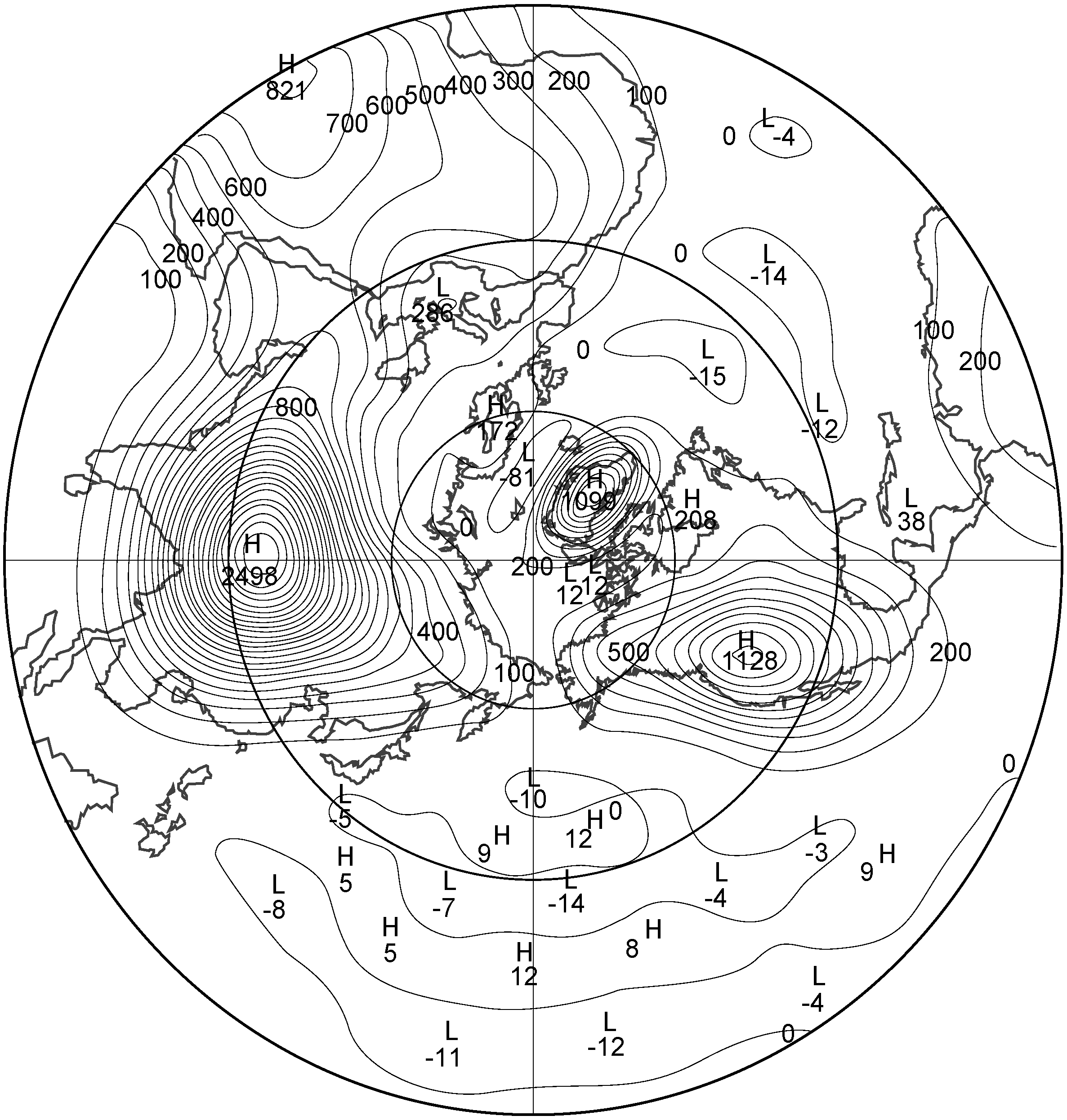
As noted earlier, the canonical equilibrium states on the generalized β-plane have the same form as on a sphere with the replacements , and . Figure 1 shows a contour plot of the Northern Hemisphere topography while in Figure 2 is shown a typical canonical equilibrium state from the study of Frederiksen and Sawford (1981) [10]. We note that the zonally asymmetric component of the 500 hPa streamfunction depicted is strongly correlated with the topography.
4. Statistical closure equations for homogeneous turbulence
The canonical equilibria discussed in the Introduction and in section 3. are stationary solutions of fundamentally based statistical dynamical closures such as the EDQNM, DIA, LET, SCFT and, in the
![Entropy 10 00635 g001]() presence of topography and mean fields, the QDIA closure. In this section, we discuss how homogeneous turbulence may be simulated through DNS, summarize the DIA closure equations and point out the relationships between the DIA, LET and SCFT for homogeneous turbulence.
presence of topography and mean fields, the QDIA closure. In this section, we discuss how homogeneous turbulence may be simulated through DNS, summarize the DIA closure equations and point out the relationships between the DIA, LET and SCFT for homogeneous turbulence.
Figure 1.
Northern Hemisphere topography in meters.
Homogeneous turbulence may be simulated with the barotropic vorticity Eq. (8a) but with and ; then with no mean forcing and with zero mean vorticity, , we expect to be able to simulate homogeneous turbulence in viscous decay simulations and in forced dissipative experiments with homogeneous random forcing and viscosity. The β-effect will result in anisotropic spectra while with isotropic spectra will result if the random forcing is isotropic. The spectral barotropic equation is again given by Eq. (13) but with , and the topographic term missing.
4.1. The homogeneous DIA closure equations
The DIA closure equations were derived by Kraichnan (1959) [42] for homogeneous turbulence and have been reviewed by McComb (1990) [65]. A recent simple derivation for two-dimensional turbulence, following Kraichnan’s approach, is given by Frederiksen (2003) [72]. Here we very briefly summarize the DIA equations for two-dimensional and Rossby wave turbulence.
We consider an ensemble of flows described by the barotropic vorticity equation that now takes the form
![Entropy 10 00635 g002]() where is a dissipation operator, such as where is the bare viscosity, although we shall also consider more general forms, and is the bare forcing. Equations (12) again hold for the doubly periodic domain. The resulting spectral form of the vorticity equation is
where is defined in Eq. (14). Also, is defined in Eq. (21a) and the interaction coefficients are now simply defined by
The DIA is derived using renormalized perturbation theory applied to the barotropic vorticity equation Eq. (46) and to an equation for the response function. The response function
measures the change in vorticity due to an infinitesimal change in the force. Infinitesimal perturbations in the forcing, in Eq. (46), produce changes in the vorticity determined by
Consequently, the response function satisfies the equation
The response function is a Green’s function that can be used to write the solution to Eq. (49) in the form
where is a dissipation operator, such as where is the bare viscosity, although we shall also consider more general forms, and is the bare forcing. Equations (12) again hold for the doubly periodic domain. The resulting spectral form of the vorticity equation is
where is defined in Eq. (14). Also, is defined in Eq. (21a) and the interaction coefficients are now simply defined by
The DIA is derived using renormalized perturbation theory applied to the barotropic vorticity equation Eq. (46) and to an equation for the response function. The response function
measures the change in vorticity due to an infinitesimal change in the force. Infinitesimal perturbations in the forcing, in Eq. (46), produce changes in the vorticity determined by
Consequently, the response function satisfies the equation
The response function is a Green’s function that can be used to write the solution to Eq. (49) in the form
Figure 2.
500 hPa Northern Hemisphere zonally asymmetric component of streamfunction for a canonical equilibrium state with strong correlation with the topography.
Figure 2.
500 hPa Northern Hemisphere zonally asymmetric component of streamfunction for a canonical equilibrium state with strong correlation with the topography.

The DIA is a non-Markovian theory that provides an approximate solution, at second order, to the moment or cumulant hierarchy, discussed in the Introduction. Kraichnan termed it the direct interaction approximation since he regarded his methodology as an expansion in terms of the complexity of modal interactions that occur through the nonlinearity of the dynamical equations. It contains no arbitrary parameters, conserves the same quadratic invariants as the original dynamical equations, and is realizable. It represents a major milestone in the development of turbulence theory.
The DIA consists of equations for the renormalized response function,
and a renormalized two-time second-order cumulant
where
Here, since and since . As well, the single-time cumulant satisfies the equation
since
In the above equations we may identify physical processes with each of the integral terms. Specifically
can be identified as nonlinear damping and noise terms respectively. The Eulerian DIA has been found to compare very closely to ensemble averages of direct numerical simulations in the energy containing ranges of large scales for both two- and three-dimensional turbulent flows. However, at high Reynolds number the Eulerian DIA leads to power laws that differ slightly from the energy and enstrophy cascading power laws. This is due to the inability of the DIA to distinguish between intrinsic distortion and convection (advection) effects. A simple way to overcome this problem is to localize the eddy transfers in wavenumber space since this can be shown to yield inertial range power law behavior consistent with the phenomenology of Kolmogorov (Kraichnan (1964) [90]). In the case of isotropic two-dimensional turbulence Frederiksen & Davies (2004) [67] find good agreement between DNS and their regularized DIA (RDIA) for which the replacements
are made in the response function and two-time cumulant equations but not in the single-time cumulant equation. Here Θ is the Heavyside step function and α is an empirically determined parameter. Furthermore, the regularization parameter is almost universal for both homogeneous (Frederiksen & Davies (2004) [67]) and inhomogeneous turbulence (O’Kane & Frederiksen (2004, 2008a) [71, 88]) with good agreement, even at the small scales, between the closures and DNS for . This regularization procedure corresponds to an empirical renormalization of the bare vertex or interaction coefficient.
4.2. Homogeneous SCFT and LET closure theories
The SCFT closure of Herring (1965, 1966) [43, 44] and the LET closure of McComb (1974, 1992) [45, 46] are non-Markovian Eulerian closure theories of homogeneous turbulence that are closely related to Kraichnan’s (1959) DIA [42]. They were formulated independently but in retrospect the SCFT and LET closure equations may be formally obtained from the DIA by invoking the fluctuation-dissipation theorem (FDT, Kraichnan (1959b) [48], Carnevale & Frederiksen (1983) [51]) out of strict statistical mechanical equilibrium as noted by Frederiksen, Davies & Bell (1994) [52]. The FDT states that
where is the Heavyside step function that vanishes for and is otherwise unity.
The FDT provides an additional relationship between the two-time cumulant and the response function and the single-time cumulant. For the SCFT, the equations are identical to the homogeneous DIA equations but the FDT equation replaces the prognostic equation for the two-time cumulant. For the LET the FDT relation instead replaces the response function equation.
5. Vorticity equation and DIA closure on the sphere
Next, we consider the problem of determining self-consistent subgrid-scale parameterizations based on closures. Since the aim is to apply these to atmospheric circulation models the formulation is developed in spherical geometry.
In spherical geometry the barotropic vorticity equation takes the same form as in Eq. (8a) and the relation between the vorticity and streamfunction is as for planar geometry, , but the Laplacian is now for spherical geometry. If we non-dimensionalize the equations by taking a (the earth’s radius) and (the inverse of the earth’s angular velocity) as length and time scales then the Jacobian is again given by Eq. (8b) but with x replaced by λ, the longitude, and y replaced by μ, the sine of the latitude. We shall use a slightly more general formulation of the dissipation than that in previous sections.
The corresponding spectral equation can be obtained by expanding each of the functions in spherical harmonics; for example
where m is zonal wavenumber, n is total wavenumber, T is the triangular truncation wavenumber, and are orthonormalized Legrendre functions. Now let
Then the spectral equation for homogeneous turbulence is
where
and
Again, since and since . Also, β represents the beta effect on the sphere, which with the current scalings, would take value 2 for the atmosphere but we shall primarily be interested in the case applicable to isotropic turbulence.
In spherical geometry, the DIA closure for homogeneous turbulence is again given by the equations described in Eqs. (52) but with the interaction coefficient given by Eq. (59a) and the Kronecker delta function Eq. (59b) replacing that of Eq. (21b) in Eq. (13) and in the viscous damping term. The selection rules on the total wavenumbers for non-zero interaction coefficients are given in Eq. (2.3) of Frederiksen and Sawford (1980) [8]. In the following sections we shall also specialize to isotropic turbulence for which the statistics of the cumulants and response functions only depend on rather than on .
6. EDQNM closure on the sphere
The time-history integrals associated with the non-Markovian DIA closure reflect memory effects associated with turbulent eddies. Other non-Markovian closure theories such as the SCFT and LET closures have very similar performance to the DIA closure. The SCFT and LET closures replace either the second-order two-time cumulant or the response function with the fluctuation dissipation theorem (FDT). Unlike quantum field theories which deal with Hermitian operators, classical systems tend not to be self-adjoint and the FDT in general only applies at canonical equilibrium (Kraichnan, (1959b) [48], Deker and Haake (1975) [50], Carnevale and Frederiksen, (1983) [51] and references therein). Nevertheless, as noted above it appears to be a reasonable approximation more generally.
For isotropic turbulence with , the non-Markovian DIA closure can be simplified to a Markovian closure called the eddy-damped quasi-normal Markovian (EDQNM) closure by replacing the equation for the two-time cumulant (Eq. (52b)) by a modified form of the FDT in Eq. (54),
and assuming an exponential decay form for the response functions
Here, the eddy damping is given by the empirical form
(Frederiksen and Davies (1997) [57]) that generalizes to spherical geometry the expressions of Orszag (1970) [54] and Leith (1971) [55]. This form of the eddy damping is consistent with the enstrophy cascading inertial range power law of two-dimensional turbulence. It is found that taking gives good comparison with DNS.
The single-time cumulant equation (Eq. (52f)) then reduces to the ordinary differential equation
We have also specialized to white noise forcing for which
so that, from Eqs. (52e) and (52f),
The nonlinear damping and nonlinear noise then reduce to
We note that the nonlinear noise is positive. The time-history integrals can be calculated analytically to determine the triad relaxation time as
with
Here the summations over and are determined by
7. Adiabatic invariants, zonalization and vortex condensation.
Atmospheric general circulation models (GCM’s) when integrated from observed initial conditions tend to develop significant errors due to a tendency to gain zonal kinetic energy at the expense of eddy kinetic energy (Hollingsworth et al. (1987) [167]). In addition, the distribution of the simulated kinetic energy as a function of zonal wavenumber also displays a marked dependence on horizontal resolution. Manabe et al. (1979) [117]) described this dependence noting that the large-scale kinetic energy increases with increasing resolution, while the energy at the smaller scales drops. Similar qualitative changes in energy spectra with horizontal resolution were found in early studies with the barotropic vorticity equation and were analysed in terms of statistical mechanical equilibrium spectra by Frederiksen and Sawford (1980) [8]. This sensitivity of model atmospheric circulations and energy spectra to resolution and dissipation parameterizations has been an ongoing issue with GCMs (Laursen & Eliasen (1989) [118], Koshyk and Boer (1995) [119], Kaas et al. (1999) [120], Frederiksen et al. (2003) [121]).
Frederiksen, Dix & Kepert (1996) [28] (hereafter FDK96) examined the dependence of kinetic energy spectra of global atmospheric flows on varying horizontal resolution, dissipation operators, topography and differential rotation (the β-effect) both in a barotropic model and in a multi-level GCM. They found that to a large extent the behavior of the spectra with varying resolution, and surprisingly with varying dissipation, could be related to the spectra of canonical equilibrium spectra. FDK96 demonstrated that in order for the larger scale energy spectra to be resolution independent significantly more sophisticated representations of the unresolved turbulent eddies than the typical and operators were required.
Frederiksen, Dix & Kepert (1996) [28] also re-examined the role of the β-effect and Rossby waves in producing anisotropic spectra and the formation of zonal jets. They considered the statistics of Rossby wave turbulence on the sphere using the EDQNM equations of section 6 (but with cumulants for anisotropic turbulence having arguments rather than ). In the presence of Rossby waves the asymptotic form of the triad relaxation time takes the form
by analogy with the planar geometry case (Holloway & Hendershott (1977) [109]). Here, are the Rossby wave frequencies of Eq. (58) and the eddy damping satisfies Eq. (62). Consider now the case where energy and enstrophy are injected, or have large amplitudes, at intermediate wavenumbers. The EDQNM equation (63) will then tend to send some of the energy to larger scales and the enstrophy to smaller scales with the transfers affected by the triad relaxation time in Eq. (69). This transfer will be reduced for Rossby waves having large intrinsic frequencies and these are the large scale waves that are meridionally elongated as seen from Eq. (58). On the other hand for the zonal components the Rossby wave frequencies are zero, the transfer is not impeded by the intrinsic frequencies, and this means that some of the energy that should have gone to the large scale Rossby waves instead goes to the zonal flow to form strong jets.
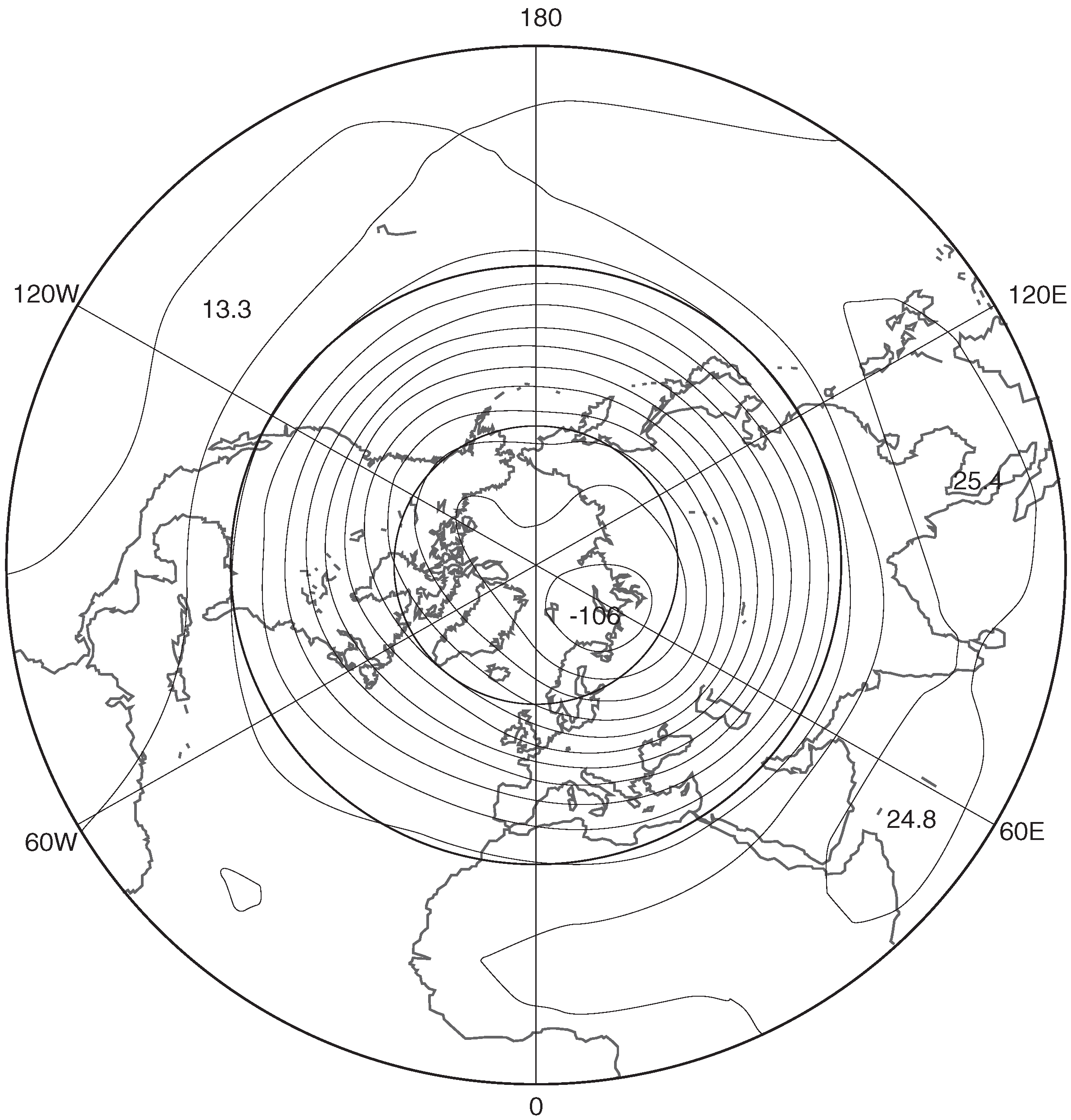
FDK96 also presented a canonical equilibrium model that captures the essential mechanism of the zonalization process. They supposed that the larger-scale Rossby waves could be regarded as adiabatic invariants that were unchanged while the zonal flow and other intermediate and small-scale eddies are allowed to equilibrate. The zonalization that results with adiabatic invariants compared with the standard canonical equilibrium spectrum where all eddies interact is demonstrated in Figure 3 (Figure 3 of FDK96). Here the canonical equilibrium energy spectra are shown for four choices of the large-scale invariants and compared with the standard equilibrium spectrum. The results use the observed 500 hPa streamfunction for 22 January 1979 as initial conditions and the spectra are calculated at rhomboidal 15 truncation. Starting from the same initial conditions FDK96 performed a series of simulations with the barotropic vorticity equation with and without the β-effect and with a dissipation operator acting only on the outer rhomboid in spectral space. Figure 4 (taken from Fig 8c of FDK96) shows the Northern Hemisphere 500 hPa streamfunction after 30 days of evolution for the case with . It is evident that the initial wavy flow (not shown) has condensed into a single circumpolar vortex; the process is somewhat analogous to Boson condensation in an ideal Bose gas. In contrast, for a corresponding simulation with the flow maintains more large-scale wave structures out to day 30 (Figure 8e of FDK96).
The results of FDK96 highlight the desirability of developing subgrid-scale parameterizations of turbulent eddies, in particular dissipation operators, that can maintain the same large-scale energy spectra with varying horizontal resolution. In the following sections we discuss subgrid modeling methods based on statistical closures with such capabilities.
8. Subgrid-scale parameterizations
Next, we examine how to establish self-consistent subgrid-scale parameterizations when the resolution is reduced from triangular truncation T to where is the triangular truncation wavenumber
![Entropy 10 00635 g003]() of the resolved scales. We define the set of resolved scales by
and the set of subgrid-scales by
Then, the nonlinear damping and nonlinear noise due to the resolved scales (respectively subgrid-scales) are given by Eqs. (65) and (66), with subscript (respectively ) for (respectively ).
of the resolved scales. We define the set of resolved scales by
and the set of subgrid-scales by
Then, the nonlinear damping and nonlinear noise due to the resolved scales (respectively subgrid-scales) are given by Eqs. (65) and (66), with subscript (respectively ) for (respectively ).
Figure 3.
Comparison of standard canonical equilibrium kinetic energy spectrum as a function of m for R15 truncation with cases where different large-scale components are treated as adiabatic invariants, namely, 1) components with ; 2) components with ; 3) components with ; 4) components with and (0,2). Note is plotted at .
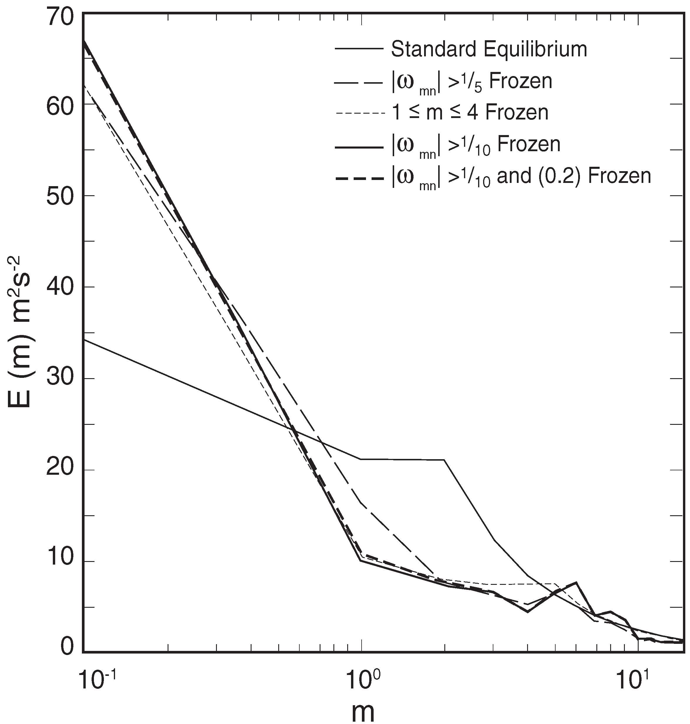
Figure 4.
Northern Hemisphere 500 hPa streamfunction (in ) on day 30 for a barotropic model simulation at rhomboidal wavenumber 15 truncation with dissipation and a beta-effect corresponding to . In this simulation an initial complex wavy flow evolves into a single circumpolar vortex.
Figure 4.
Northern Hemisphere 500 hPa streamfunction (in ) on day 30 for a barotropic model simulation at rhomboidal wavenumber 15 truncation with dissipation and a beta-effect corresponding to . In this simulation an initial complex wavy flow evolves into a single circumpolar vortex.
8.1. The EDQNM Closure
For the EDQNM closure, the equation for (twice) the enstrophy components of the resolved scales can then be written in the form
It is then clear that modifies the bare viscous damping and modifies the random forcing variance. As noted in Eq. (66), is positive and corresponds to an injection of enstrophy from the subgrid scale eddies to the resolved scales; that is, it represents stochastic backscatter. We therefore define the eddy drain viscosity
the renormalized viscosity
the stochastic backscatter
and the renormalized noise variancex
The injection of enstrophy due to the stochastic backscatter term may contribute to the growth of instabilities, which may be suppressed in lower resolution LES unless the flow is randomly forced or suitably chaotic (Leith (1990) [126], Piomelli et al. (1991) [168]). Most atmospheric circulation models have however not accounted for the stochastic backscatter term, but have tried to account for the differences between the drain and injection terms by an effective or net viscosity. This may be achieved as in Frederiksen and Davies (1997) [57] by defining a (negative) eddy backscatter viscosity through
so that,
The net eddy viscosity is defined by
and the renormalized net viscosity by
8.2. The DIA closure
For the DIA closure the viscosities again have the relationships defined for the EDQNM closure but with the eddy drain viscosity defined by
the stochastic backscatter by
and the eddy backscatter viscosity by
(Frederiksen and Davies (1997) [57]). Here the integral terms of course come from the integrals in the DIA closure equation.
Figure 5.
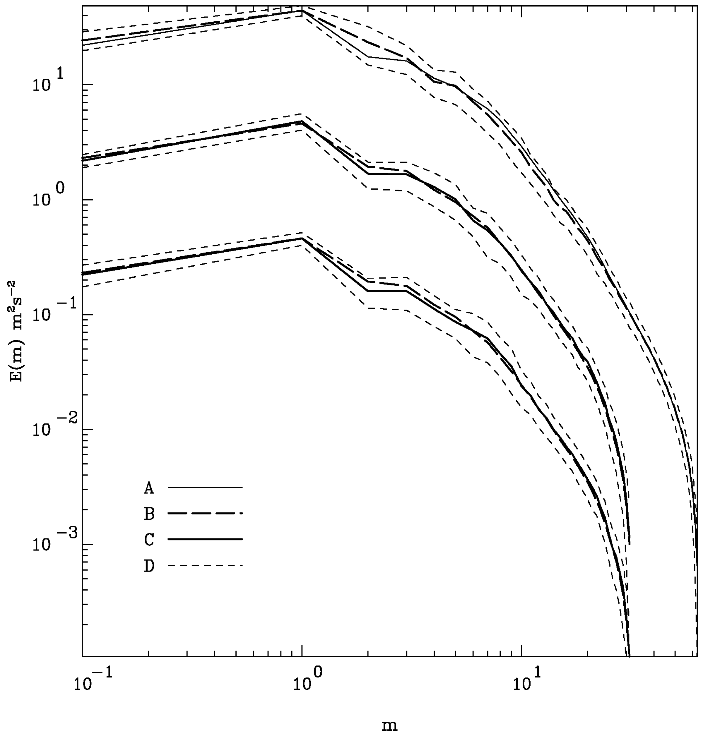
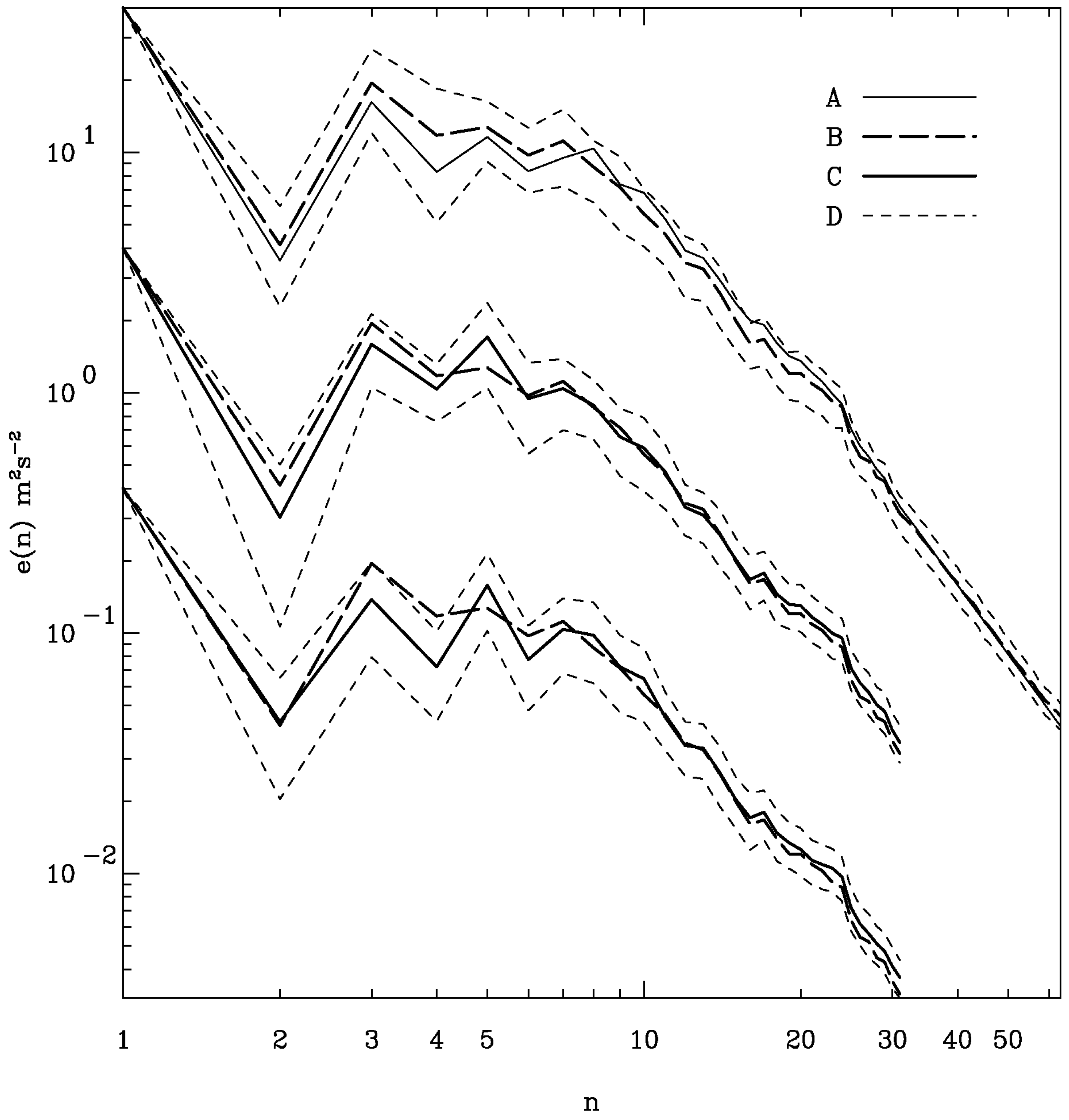
Kinetic energy spectra in for (A) isotropized January 1979, (B) DNS at T63, (C) LES at T31, and (D) for DNS or LES. LES results with EDQNM-based renormalized stochastic backscatter and renormalized viscosity () and LES with EDQNM-based renormalized net viscosity (). Note that results for are plotted at . Integrations use .
Figure 5.
Kinetic energy spectra in for (A) isotropized January 1979, (B) DNS at T63, (C) LES at T31, and (D) for DNS or LES. LES results with EDQNM-based renormalized stochastic backscatter and renormalized viscosity () and LES with EDQNM-based renormalized net viscosity (). Note that results for are plotted at . Integrations use .
9. Comparisons of DNS and LES with subgrid-scale parameterizations
Frederiksen and Davies (1997) [57] compared DNS with LES at various resolutions and including dynamic subgrid-scale parameterizations. They focused on DNS simulations which reproduced the observed January 1979 isotropized kinetic energy spectrum as a statistically stationary spectrum in the presence of random forcing and dissipation. The DNS runs have been performed at triangular T63 resolution with the dissipation taken as a linear combination of surface drag and a Laplacian dissipation for which the nondimensional bare viscosity takes the form
The drag corresponds to , or an e-folding decay time of 15.6 days, and the Laplacian contribution corresponds to in dimensional units.
To determine the random forcing variance spectrum needed to balance the dissipation, the steady state EDQNM equation is used as follows. With the enstrophy components specified by the T63 January 1979
![Entropy 10 00635 g006]() isotropic spectrum, and the triad relaxation time given by the stationary form in Eq. (67b), must be specified by
for a steady state solution to Eq. (63). The bare viscosity in Eq. (75) and bare forcing specified by Eq. (76) (with ) when used in DNS of the barotropic vorticity equation also produce a statistically steady state which is very close to the January 1979 spectrum. This is shown in Fig. 5 and Fig. 6 (redrawn from Frederiksen and Davies, (1997) [57]) which, at T63, compare the results of a DNS run (including rotation ) averaged over the last 100 days of a 150-day simulation with the January 1979 spectrum. Figure 5 shows the dimensional zonal wavenumber kinetic energy spectrum while Figure 6 shows the dimensional total wavenumber kinetic energy spectrum . Also shown are these spectra ± the standard deviations and . The zonal wavenumber spectra are in close agreement at most scales while for the total wavenumber spectra the agreement at the largest scales, where there are few m components to average over and where the eddy turn-over time is long, is not as good as at small scales. The DNS spectra in Fig. 5 & Fig. 6, or, almost equivalently, the T63 January 1979 spectra, are regarded as the benchmark or truth against which LES at lower resolution are to be compared.
isotropic spectrum, and the triad relaxation time given by the stationary form in Eq. (67b), must be specified by
for a steady state solution to Eq. (63). The bare viscosity in Eq. (75) and bare forcing specified by Eq. (76) (with ) when used in DNS of the barotropic vorticity equation also produce a statistically steady state which is very close to the January 1979 spectrum. This is shown in Fig. 5 and Fig. 6 (redrawn from Frederiksen and Davies, (1997) [57]) which, at T63, compare the results of a DNS run (including rotation ) averaged over the last 100 days of a 150-day simulation with the January 1979 spectrum. Figure 5 shows the dimensional zonal wavenumber kinetic energy spectrum while Figure 6 shows the dimensional total wavenumber kinetic energy spectrum . Also shown are these spectra ± the standard deviations and . The zonal wavenumber spectra are in close agreement at most scales while for the total wavenumber spectra the agreement at the largest scales, where there are few m components to average over and where the eddy turn-over time is long, is not as good as at small scales. The DNS spectra in Fig. 5 & Fig. 6, or, almost equivalently, the T63 January 1979 spectra, are regarded as the benchmark or truth against which LES at lower resolution are to be compared.
Figure 6.
As in Figure 5 for shown as (A), (B), (C) and shown as (D).
Figure 6.
As in Figure 5 for shown as (A), (B), (C) and shown as (D).
The various EDQNM subgrid-scale terms defined in section 9., are shown in Fig. 7 & Fig. 8 (redrawn from Figure 3b & d of Frederiksen and Davies (1997) [57]) for the case when the initial T63 January 1979 spectrum is truncated back to T31. Figure 7 depicts the eddy viscosities , and while Figure 8 shows the net dissipation function . We note that these subgrid-scale
![Entropy 10 00635 g007]() parameterizations all have a cusp behavior at the smallest scales as is also characteristic of eddy viscosity parameterizations for three-dimensional turbulence in Cartesian geometry (Kraichnan (1976) [122], Chasnov (1991) [127]). Very similar subgrid-scale parameterizations are obtained when the January 1979 spectrum is truncated back to other lower resolutions as shown at T15 in Figure 4 of Frederiksen and Davies (1997) [57].
parameterizations all have a cusp behavior at the smallest scales as is also characteristic of eddy viscosity parameterizations for three-dimensional turbulence in Cartesian geometry (Kraichnan (1976) [122], Chasnov (1991) [127]). Very similar subgrid-scale parameterizations are obtained when the January 1979 spectrum is truncated back to other lower resolutions as shown at T15 in Figure 4 of Frederiksen and Davies (1997) [57].
Figure 7.
EDQNM nondimensional subgrid-scale parameterizations for T31. Shown are viscosities corresponding to (A) , (B) , and (C) .
Figure 7.
EDQNM nondimensional subgrid-scale parameterizations for T31. Shown are viscosities corresponding to (A) , (B) , and (C) .
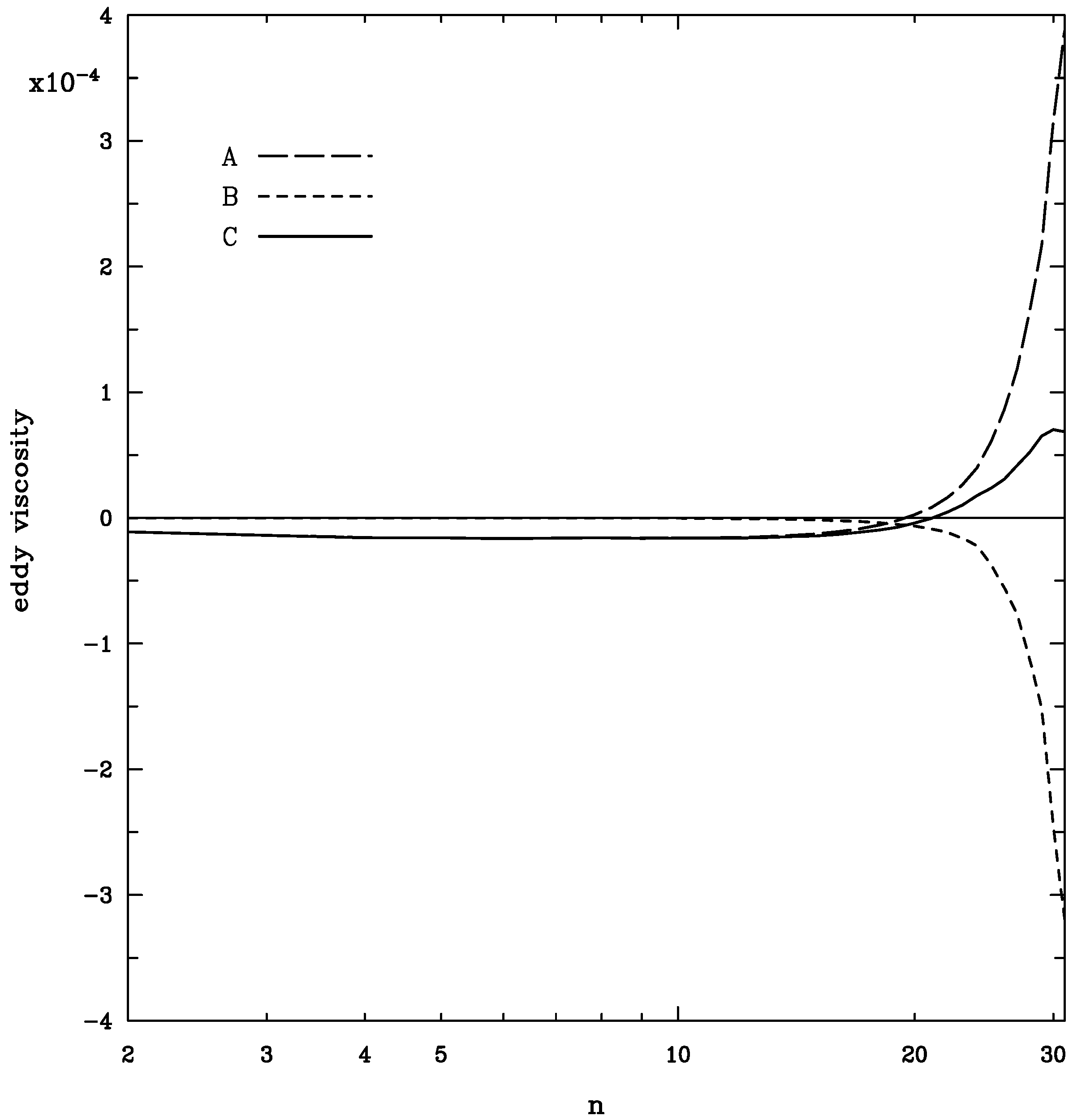
Fig. 5 & Fig. 6 also compares the spectra of LES using the renormalized viscosity and renormalized random forcing at resolutions T31 and T15. Again the kinetic energy spectra shown are averaged over the last 100 days of 150-day simulations. The diagrams also show the spectra ± the standard deviation and and the energy spectra of the T63 DNS, and January 1979 observations, truncated back to T31 or T15. For the zonal wavenumber spectra, there is good agreement between the LES kinetic energies at T31 and T15 and both the DNS and January 1979 results truncated to the resolution of the LES. For the total wavenumber spectra, the agreement between LES and DNS or January 1979 kinetic energies is good at the smaller scales; at the larger scales there are some deviations, presumably because of the few m components to average over and the long eddy turn-over times.
Frederiksen and Davies (1997) [57] show that the generally good agreement between DNS and LES using the EDQNM based renormalized viscosity and renormalized noise forcing is also found if the EDQNM based renormalized net viscosity is used instead or if the corresponding very similar DIA
![Entropy 10 00635 g008]() based parameterizations are employed. This is also the situation in the presence of a differential rotation speed characteristic of the earth. They also find that the comparison between DNS and LES is much better than when a number of ad hoc viscosity parameterizations are used in the LES.
based parameterizations are employed. This is also the situation in the presence of a differential rotation speed characteristic of the earth. They also find that the comparison between DNS and LES is much better than when a number of ad hoc viscosity parameterizations are used in the LES.
Figure 8.
As in Figure 7 for .
Figure 8.
As in Figure 7 for .

10. Closures and subgrid-scale terms for inhomogeneous geophysical flows
In this section, we review the QDIA closure theory ([88, 98, 99] and present analytical expressions for the various subgrid-scale terms entering the equations for the mean and fluctuating components of the vorticity within the barotropic vorticity equation for inhomogeneous turbulent flow over topography.
10.1. QDIA closure equations
The QDIA closure was formulated by Frederiksen (1999) [98] (hereafter F1999) for directly calculating the statistics of nonequilibrium barotropic flows interacting with inhomogeneous turbulence and topography. It was used to provide a general theoretical framework for subgrid-scale parameterizations of the eddy-topographic force, eddy viscosity and stochastic backscatter. Numerical implementation and extensive testing of the QDIA closure was performed by O’Kane & Frederiksen (2004) [88] using an efficient restart method and the theory and numerics were extended by Frederiksen & O’Kane (2005) [99] to incorporate differential rotation and Rossby waves. Recently the QDIA closure has also been applied to predictability studies of atmospheric flows (O’Kane & Frederiksen (2008a) [71]) and to atmospheric data assimilation (O’Kane & Frederiksen (2008c) [101] in this issue).
In this section we briefly state the closure equations required for a discussion of the subgrid calculations and refer the reader to the articles quoted above for more details. Let us suppose we have an ensemble of flows satisfying Eq. (13) where and 〈〉 denotes mean and denotes fluctuation about the mean. Also, where . The equations for the ensemble mean and the fluctuation can then be written in the form:
Here the two-point cumulant is defined by
where and both range over the whole plane including the zero vector that represents the large scale flow. Throughout we will use the abbreviations
The mean-field closure equation takes the form
The nonlinear damping is as defined in Eq. (52h) but here measures the interaction of transient eddies with the mean field while
measures the strength of the interaction of transient eddies with the topography in Eq. (81).
The equation for the diagonal two-time two-point cumulant is obtained by multiplying Eq. (78) by and using the closure expressions Eqs. (52h), (52i), (84) & (85):
Here and the nonlinear noise is as defined in Eq. (52i). Also,
are noise and dissipation terms associated with eddy-mean field and eddy-topographic interactions.
The diagonal response function, , satisfies
where
Finally, the single-time cumulant is given by
10.2. Generalized Langevin Equation
The realizability of the diagonal elements of the covariance matrix in the QDIA closure equations is underpinned by the fact the closure has an exact stochastic model representation. The generalized Langevin equation that reproduces the QDIA is
where
Here , where , are statistically independent random variables such that
and
where δ is the Kronecker delta function in Eq. (91).
10.3. Subgrid terms
Frederiksen (F1999) derived expressions for the subgrid-scales based on the QDIA equations and the associated Langevin equations. Here we consider the case where the resolution is reduced from to with the resolution of the resolved scales in circularly truncated wavenumber space. We define , and is the set of the subgrid scales. Thus for , one or both of these inequalities , holds. We now simply state the dynamical equations for the resolved scale vorticity including subgrid terms
where the mean subgrid tendency is given by
Here the subgrid scale eddy-topographic force and subgrid residual Jacobian are defined by
Similarly
where the fluctuating subgrid tendency is given by
Eqs. (94) and (98) are the general forms of the subgrid-scale terms including memory effects of turbulent eddies. They take a simpler form if we make the Markov assumption that and (and possibly, but not necessarily, , since does not depend on time) behave like the Dirac delta function . We define
Then the subgrid tendencies take the forms
and
Here, the eddy drain viscosities are defined by
and the eddy-topographic force is
We may also define the renormalized viscosities
and the renormalized mean and random forcings
For flow on a β-plane with differential rotation and are complex in general. Now, Eq. (93) can be written in the same form as the higher resolution Eq. (77) with the replacements , (and ). Similarly Eq. (97) can be written as in Eq. (78) with the replacements , (and ). This then completes the renormalization procedure.
11. QDIA closure based SSP’s for global atmospheric flow
As reviewed in the Introduction, since the work of Holloway (1992) [140] there have been a series of papers employing heuristic subgrid-scale parameterizations of the eddy-topographic force for oceanic circulations including in general circulation ocean models. There has as yet been no implementation of subgrid parameterizations of the eddy-topographic force in atmospheric GCMs.
In this section, we compare the QDIA closure based subgrid-scale formalism (Frederiksen (1999) [98]) with approaches based on relaxation towards canonical equilibria (Holloway (1992) [140]) and on entropy production arguments (Kazantsev et al. (1998) [155], Polyakov (2001) [156] and Holloway
(2004) [157]). In our comparisons we draw on the recent numerical results of O’Kane & Frederiksen (2008b) [100]. They calculated the QDIA based subgrid terms both for a canonical equilibrium case (including forcing and dissipation balanced at each wavenumber) and for a nonequilibrium dissipative case corresponding to observed January 1979 flow over topography. Very similar subgrid results are found with the QDIA and for the regularized QDIA with in Eq. (53). A crucial question is the relative strengths of the residual Jacobian, subgrid-scale eddy-mean field and eddy-topographic interactions for flows far from equilibrium. In the the following discussion the subgrid-scale parameterizations are calculated for circularly truncated wavenumber large eddy simulations based on the results of higher resolution direct numerical simulations. In all cases a bare non-dimensional viscosity
is used, , with length-scale , time-scale and all other parameters detailed in table 1.

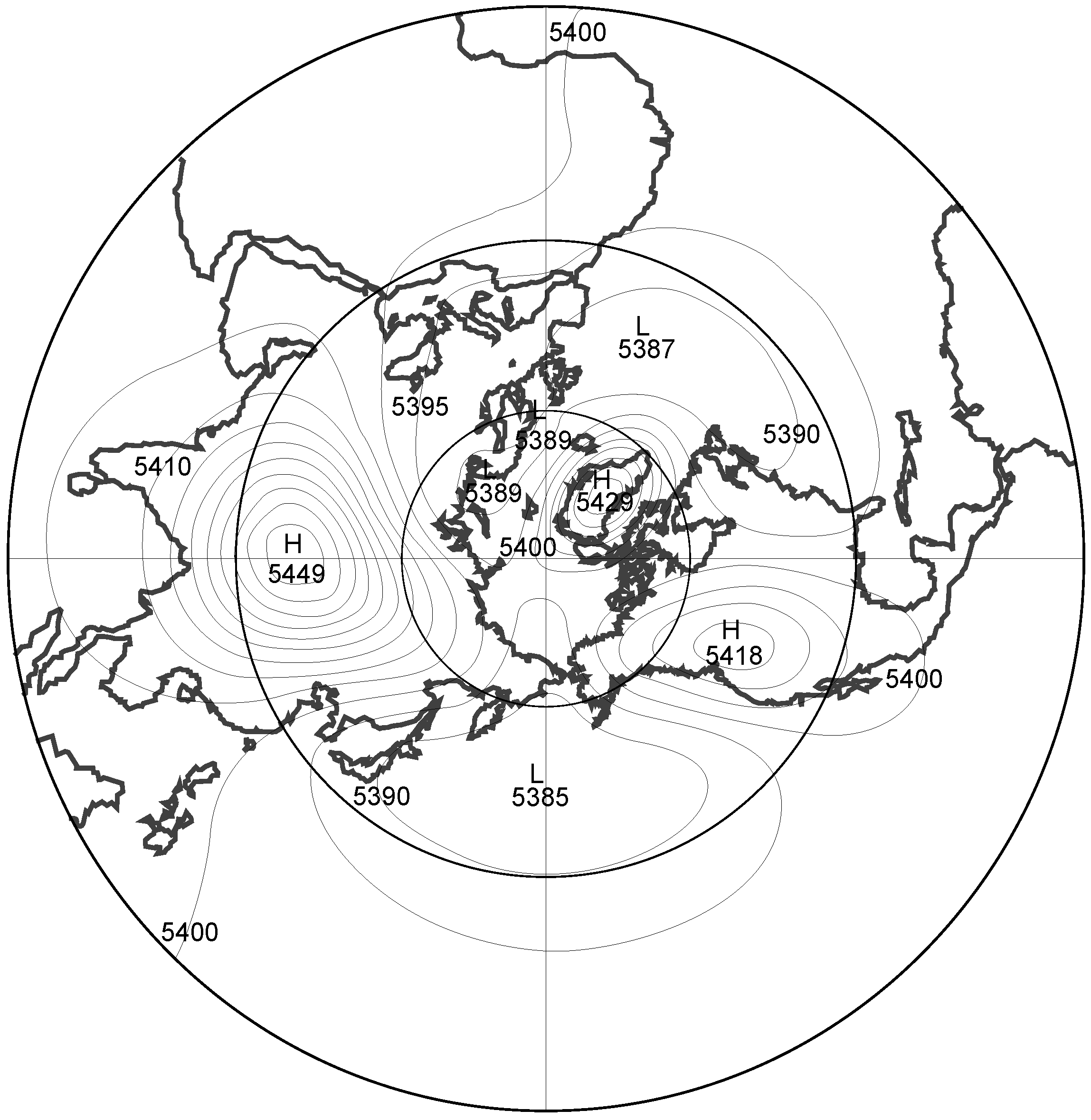
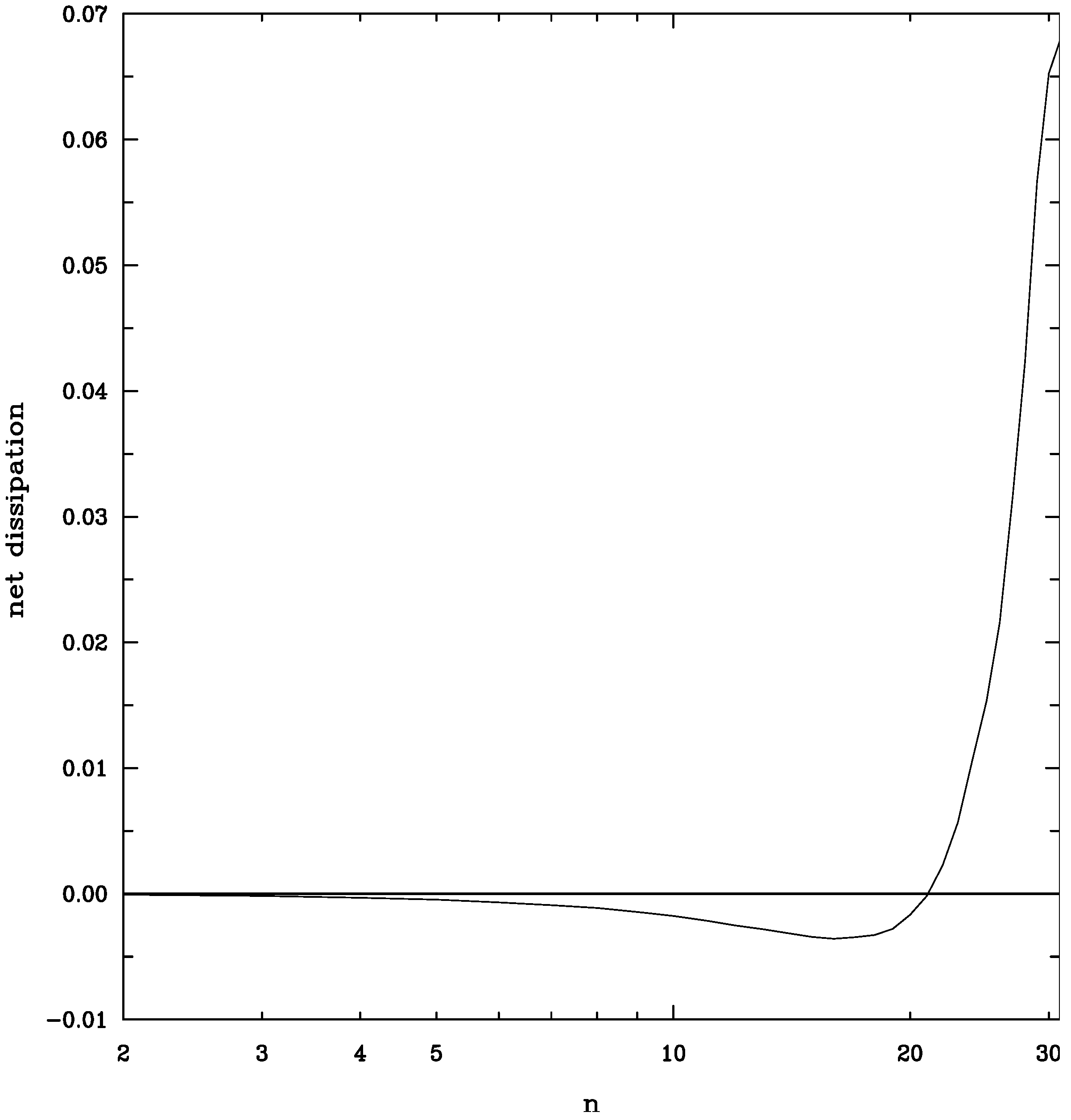
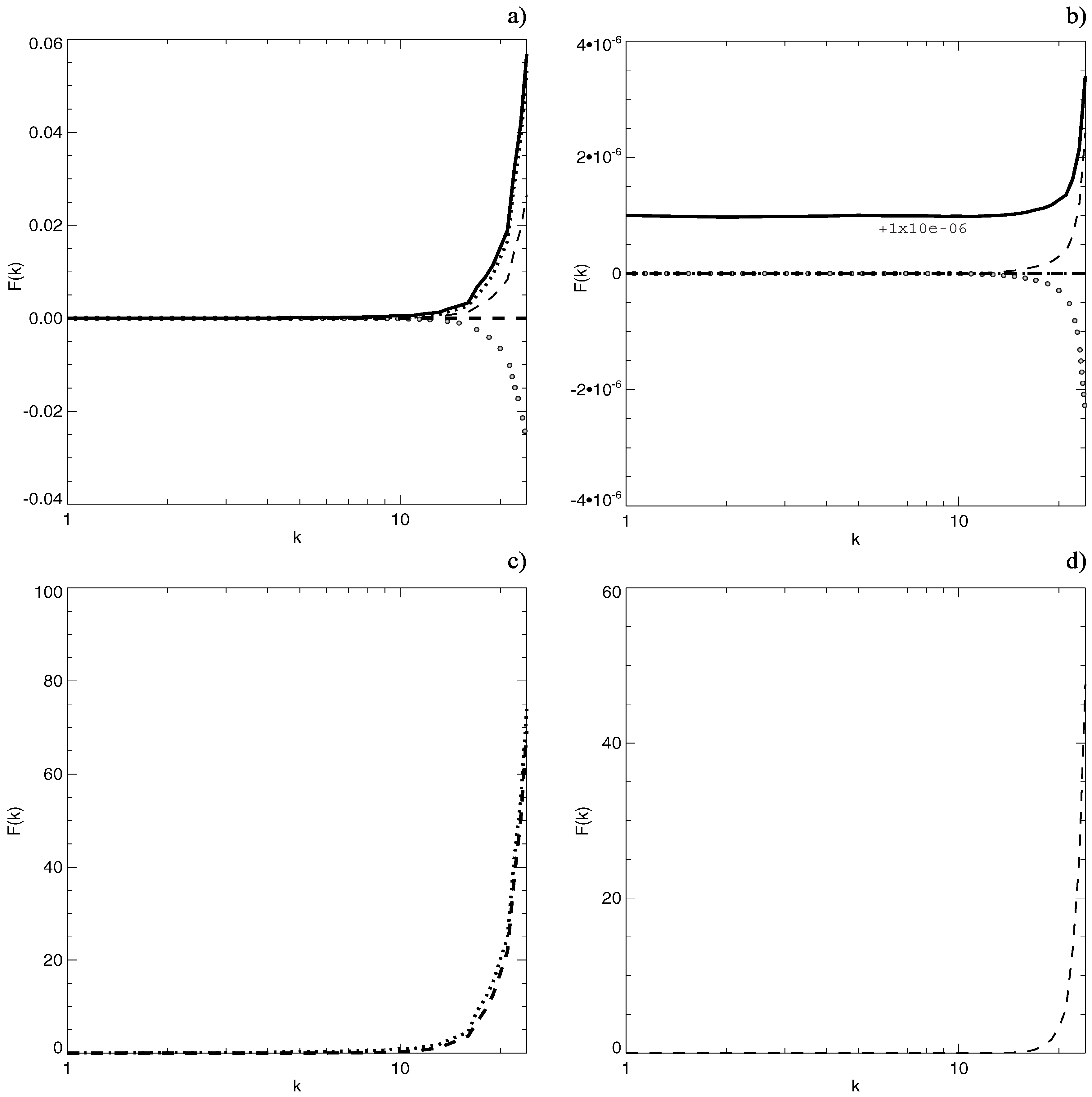
Table 1.
Parameters used in both the forced dissipative canonical equilibrium and decaying nonequilibrium cases.
11.1. Canonical equilibrium
Figure 9 shows the full integral forms of the subgrid terms in -space for the canonical equilibrium case. The physical space eddy-topographic force is shown in Figure 10 as are the zonally asymmetric component of the mean streamfunction, the mean vorticity and the global topography used in these calculations. As noted in table 1
For ease viewing, Figure 11 shows some of the spectral space subgrid terms in Figure 9 but summed over all that lie within a given radius band of unit width. These subgrid-scale terms have been calculated with an integration time of 10 hours.
We see from Figure 9 that the integral terms appearing in the single-time cumulant equation in Eq. (88) are real and homogeneous whereas the mean field subgrid terms in Eq. (81) are complex and highly anisotropic. Note that all terms balance with their counter-parts so that canonical equilibrium is exactly maintained. Fig. 9 & Fig. 10 a) clearly show that, consistent with the F1999 statistical theory,
![Entropy 10 00635 g009]() the eddy-topographic force is balanced exactly by the damping due to eddy-mean field interactions and in physical space resembles a high pass filtered form of the topography. Crucially, for the canonical equilibrium state the residual Jacobian is identically zero, as also shown in Figure 11 b). Figure 9 also clearly demonstrates that energy injection from the subgrid scales to the retained scales occurs not only in the form of stochastic backscatter due to eddy-eddy interactions but also arises due to nonlinear noise terms associated with eddy-mean and eddy-topographic interactions. These forcings balance the drain of energy from the retained to subgrid scales due to eddy-eddy, eddy-mean field and eddy-topographic dampings. Figure 11 shows that the spectra of the QDIA based subgrid terms, including the renormalized and net eddy viscosities and eddy-topographic force, are all cusp shaped at the cut-off scale. These results are consistent with corresponding subgrid terms for isotropic turbulence based on DIA and EDQNM closures and on stochastic modeling, as discussed in the Introduction. For the current inhomogeneous case this again results in the subgrid terms being of small scale and more specifically that the subgrid scale eddy-topographic force will be a high pass filtered version of the topography. Fig. 10 b) & Fig. 10 c) depict the strong correlation of both the zonally asymmetric component of the streamfunction and the mean vorticity with the topography (Figure 10 d) respectively. We have found that qualitatively similar results hold for the corresponding inviscid unforced canonical equilibrium case (not shown).
the eddy-topographic force is balanced exactly by the damping due to eddy-mean field interactions and in physical space resembles a high pass filtered form of the topography. Crucially, for the canonical equilibrium state the residual Jacobian is identically zero, as also shown in Figure 11 b). Figure 9 also clearly demonstrates that energy injection from the subgrid scales to the retained scales occurs not only in the form of stochastic backscatter due to eddy-eddy interactions but also arises due to nonlinear noise terms associated with eddy-mean and eddy-topographic interactions. These forcings balance the drain of energy from the retained to subgrid scales due to eddy-eddy, eddy-mean field and eddy-topographic dampings. Figure 11 shows that the spectra of the QDIA based subgrid terms, including the renormalized and net eddy viscosities and eddy-topographic force, are all cusp shaped at the cut-off scale. These results are consistent with corresponding subgrid terms for isotropic turbulence based on DIA and EDQNM closures and on stochastic modeling, as discussed in the Introduction. For the current inhomogeneous case this again results in the subgrid terms being of small scale and more specifically that the subgrid scale eddy-topographic force will be a high pass filtered version of the topography. Fig. 10 b) & Fig. 10 c) depict the strong correlation of both the zonally asymmetric component of the streamfunction and the mean vorticity with the topography (Figure 10 d) respectively. We have found that qualitatively similar results hold for the corresponding inviscid unforced canonical equilibrium case (not shown).
Figure 9.
Nondimensional subgrid scale terms in space entering the single-time cumulant equation (88) and the mean field equation (81) for the forced dissipative canonical equilibrium: a) , b) , c) , d) , e) , f) , g) , & . The time integration is 10 hours, ℜ denotes real part and ℑ is imaginary part.

The numerical results for subgrid-scale parameterizations described in this subsection confirm the analytical findings and general principles of the F1999 statistical theory.
Figure 10.
Figure 10. Subgrid terms in physical space for the canonical equilibrium case showing a) of the eddy-topographic force, b) the zonally asymmetric component of the mean streamfunction, c) the mean vorticity and d) the global topography. All figures are in non-dimensional units.
Figure 10.
Figure 10. Subgrid terms in physical space for the canonical equilibrium case showing a) of the eddy-topographic force, b) the zonally asymmetric component of the mean streamfunction, c) the mean vorticity and d) the global topography. All figures are in non-dimensional units.
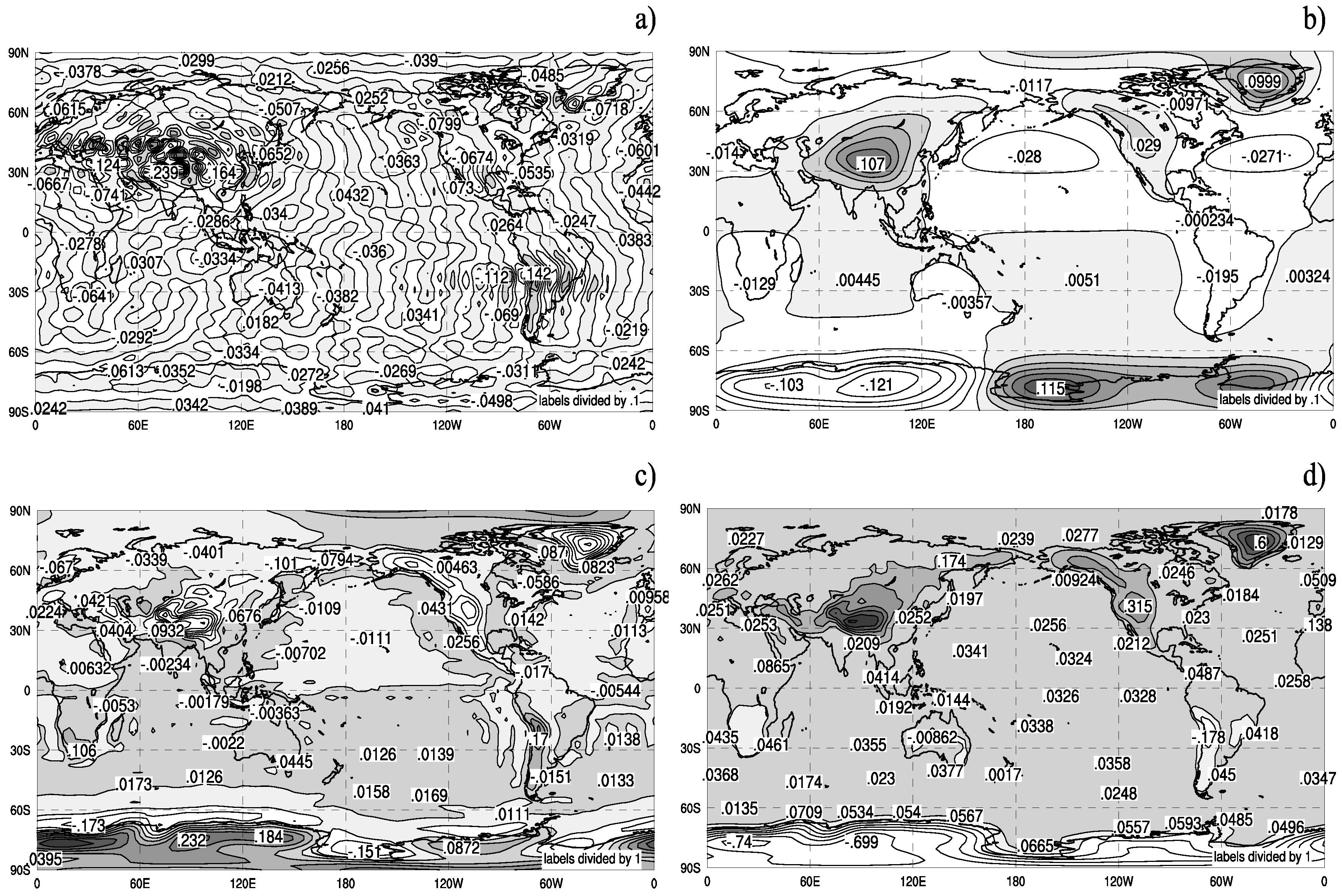
11.2. Nonequilibrium results
For general nonequilibrium flows there are unfortunately no analytic solutions and numerics must be our guide. Again we refer to the study of O’Kane & Frederiksen (2008b) [100] who considered the case of a typical 500mb January atmospheric flow over topography. They found that the subgrid contributions in the single-time cumulant equation in Eq. (88) are in general complex, prior to taking the real parts, and an imbalance between the energy injection and drain terms occurs at each wavenumber. In addition, a similar imbalance occurs between eddy-topographic, eddy-mean field and eddy-eddy interactions contributing to the mean flow. Importantly, unlike the canonical equilibrium case, the residual Jacobian not only does not vanish but makes a contribution comparable in magnitude to both the damping due to eddy-mean field interaction and to the eddy-topographic force. Fig. 10 b) & Fig. 12 a) demonstrate the differences between zonally asymmetric components of the mean streamfunctions for equilibrium and nonequilibrium flows respectively. In Figure 10 b) we see that at equilibrium the zonally asymmetric streamfunction is strongly correlated with the contours of the topography whereas the nonequilibrium case has a more complex structure with Rossby wavetrains in the mid-latitudes of the Northern Hemisphere in the band of the strong zonal jets. Figure 12 b) shows the total field for the mean streamfunction for January 1979 with strong jets in both hemispheres in the zonal winds (not shown).
Fig. 10 a) & Fig. 12 d) demonstrate the remarkable similarity in the structure of the eddy-topographic
![Entropy 10 00635 g011]()
![Entropy 10 00635 g012]() force for both cases with strong interactions occurring over the large-scale topographic structures such as the Himalayas, the Andes, Greenland and to a lesser extent the Rocky Mountains. In the nonequilibrium case (Figure 12 c) the residual Jacobian has significant contributions from both the mean-field mean-field interaction as well as the mean-field topographic interaction (not shown). Upon further investigation we have found that the quadratic mean-field terms in the residual Jacobian consist of small-scale Rossby wavetrains stretching from the Himalayas over the North Pacific. The mean-field topographic terms on the other hand have features broadly similar, but of larger scale, to those seen in the eddy-topographic force.
force for both cases with strong interactions occurring over the large-scale topographic structures such as the Himalayas, the Andes, Greenland and to a lesser extent the Rocky Mountains. In the nonequilibrium case (Figure 12 c) the residual Jacobian has significant contributions from both the mean-field mean-field interaction as well as the mean-field topographic interaction (not shown). Upon further investigation we have found that the quadratic mean-field terms in the residual Jacobian consist of small-scale Rossby wavetrains stretching from the Himalayas over the North Pacific. The mean-field topographic terms on the other hand have features broadly similar, but of larger scale, to those seen in the eddy-topographic force.
Figure 11.
Non-dimensional summed band averaged spectra for canonical equilibrium case showing a) (thin dashed), (circles), (thick dot), (thick solid), (the thick dashed line shows the sum (=0) of terms in circles + thin dashed); b) (thick dot (=0)), (thin dashed), (circles), (thick solid), (the thick dashed line shows the sum (=0) of terms in circles + thin dashed); c) (thick dashed), (thick dot); d) (thin dashed).

Figure 12.
Figure 12 a) Zonally asymmetric component of mean streamfunction for the nonequilibrium decaying January case, b) mean streamfunction, c) of residual Jacobian, d) of eddy-topographic force. All figures (non-dimensional) are after 24 hours of development.
Figure 12.
Figure 12 a) Zonally asymmetric component of mean streamfunction for the nonequilibrium decaying January case, b) mean streamfunction, c) of residual Jacobian, d) of eddy-topographic force. All figures (non-dimensional) are after 24 hours of development.
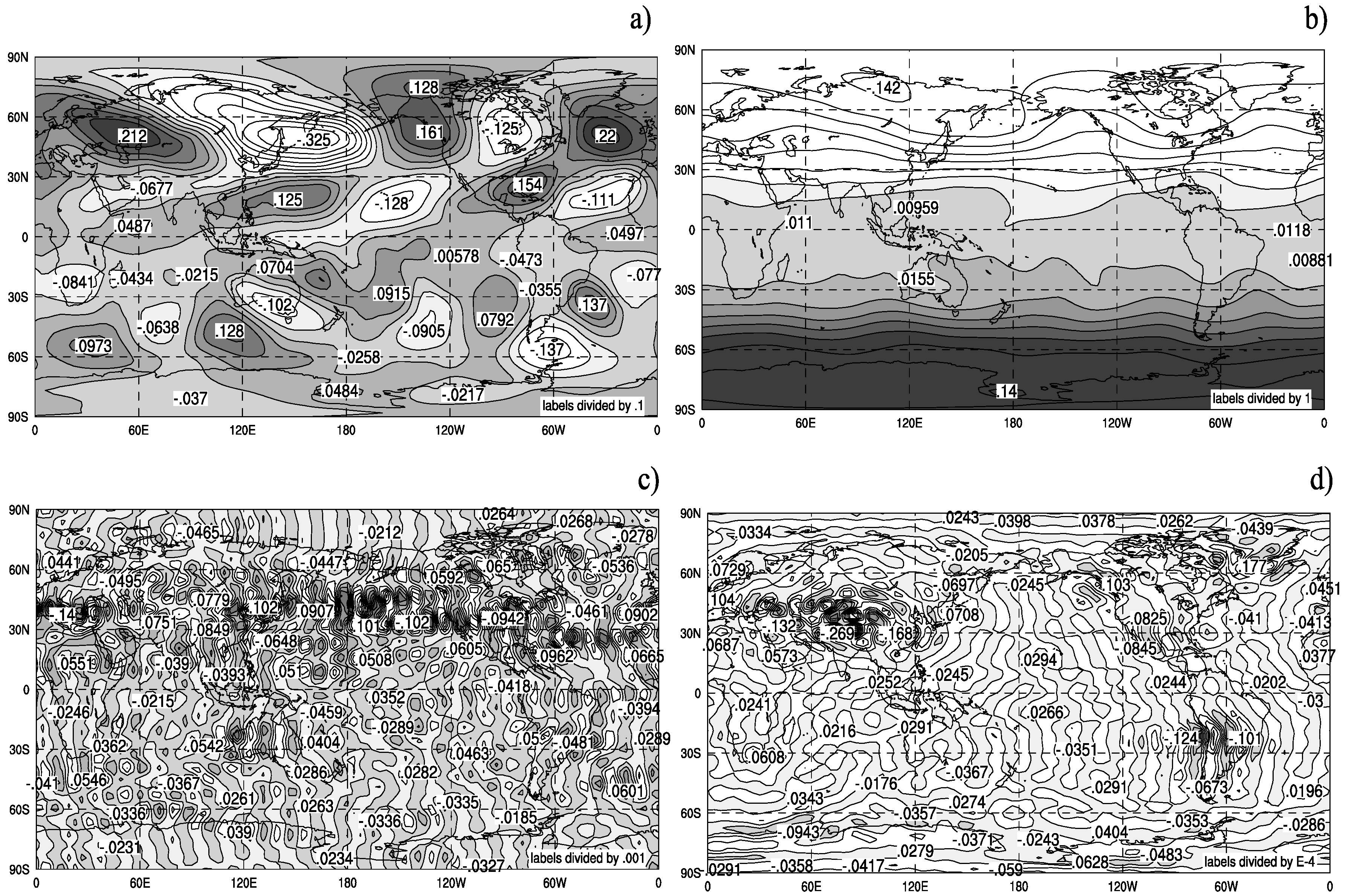
11.3. Comparison with subgrid terms obtained from entropy methods
Holloway (1992) [140] proposed that in the presence of topography the effects of subgrid-scale eddies are to relax the barotropic component of the flow towards a local canonical equilibrium rather than towards rest. Thus, he proposed that the mean subgrid tendency (Eqs. (94) and (100)) takes the form
where the eddy-topographic force
Since H1992 effectively takes , his total viscosity and Eq. (109) agrees with the F1999 equilibrium form:
Holloway (H1992) does not explicitly propose subgrid-scale parameterizations for the subgrid tendency entering the equation for the fluctuations. However, he presented and applied (e.g. Alvarez et al.(1994) [142]) his eddy-topographic stress parameterization in a framework without stochastic backscatter subgrid-scale parameterizations. As noted by Frederiksen (F1999) stochastic backscatter is essential to balance the eddy damping of the fluctuations even at canonical equilibrium. Additionally, in applications of the H1992 framework the same viscous terms are used for both the subgrid contributions to the fluctuating and mean vorticity tendencies, viz., . In contrast, F1999 shows that different damping terms balance the eddy-topographic force (Eq. (100)) and stochastic backscatter terms (Eq. (101)). Applications of the H1992 parameterization typically employ dissipation operators of the form or while the cusp shapes in Figure 11 correspond to higher order operators with peaks at smaller scales. These differences mean that will be of smaller scale than . Of course in far from equilibrium situations, such as for the January 1979 flow considered in the previous subsection, the differences between H1992 and F1999 are even more significant. Table 2 presents a comparison of the H1992 and F1999 subgrid-scale parameterizations. In particular, the F1999 expression for is in general different from the equilibrium expression in Eq. (110) and the residual Jacobian .
Kazantsev et al. (1998) [155] and Polyakov (2001) [156] have also formulated subgrid scale parameterizations for flows over topography described by barotropic and shallow water equations respectively. They use a maximum entropy production hypothesis constrained by the conserved quantities of the inviscid equations. They again obtain a contribution to the mean subgrid tendency of the form in Eq. (108) together with an ordinary Laplacian diffusion term. In their case the relaxation towards canonical equilibrium is determined to be through a simple drag term. This is in sharp contrast to the cusp shaped eddy viscosities shown in Figure 11 and in earlier closure and stochastic modeling studies. Holloway (2004) [157] has argued that his form for the mean subgrid tendency (Eq. (108)) can be obtained from a Taylor expansion of the gradient of the entropy about a canonical equilibrium solution.
The nonequilibrium statistical dynamical QDIA closure theory (Frederiksen (1999) [98]) has been extensively tested and in regularized form is in excellent agreement with results of direct numerical simulations of general mean flows interacting with inhomogeneous turbulence, Rossby waves and topography (O’Kane & Frederiksen (2004) [88] and Frederiksen & O’Kane (2005) [99]) and in predictability studies (O’Kane & Frederiksen (2008a) [71]). It allows the self consistent determination of all the subgrid terms entering the equations for the mean and fluctuating components of the dynamical fields (O’Kane & Frederiksen (2008b) [100]) both near canonical equilibrium and for nonequilibrium barotropic turbulent flows. When the streamfunction is strongly correlated with the topography (Fig. 2 and Fig. 10 b)), as occurs in parts of the ocean, relaxation towards a tuned canonical equilibrium flow may improve circulations as reviewed in the Introduction. However, for far from equilibrium systems, such as the atmosphere where the stationary Rossby waves are strongly phase shifted in relation to the topography (Figure 12 a)), the results of the general QDIA theory are needed. In future we plan to develop and apply the QDIA closure theory for more complex baroclinic flows.
Table 2.
Comparison of the F1999 (Markovianized) and H1992 subgrid-scale parameterization schemes. Here is the renormalized viscosity of F1999 and is the total viscosity of H1992.
12. Summary
We have reviewed the development of the theory of statistical mechanical equilibrium states, corresponding to maximum entropy, and their applications for understanding the dynamics of geophysical flows. Maximum entropy states have been shown to be closely related to minimum enstrophy states that are nonlinearly stable in the sense of Arnold. Both of these end states of inviscid dynamics have yielded significant insights into the behavior of geophysical flows, of atmospheric circulation models and been used to explain qualitative features of ocean circulations even in the presence of forcing and dissipation.
More generally theoretical models of nonequilibrium statistical states are needed for quantitative understanding of forced dissipative flows. Turbulent closure models based on renormalized perturbation theory provide the requisite tools for such analyses. We have reviewed their development from the pioneering works of Kraichnan, Herring and McComb, who formulated non-Markovian closures for homogeneous turbulence, to recent formulations and computations with closures for inhomogeneous Rossby wave turbulence interacting with general mean flows and topography.
Closure theories form a natural basis for a systematic approach to dynamical subgrid-scale parameterizations needed for large eddy simulations of geophysical flows. We have reviewed recent advances in the formulation and application of subgrid-scale parameterizations of eddy viscosity, stochastic backscatter and eddy-topographic force. We have contrasted results based on ad hoc formulations, on ideas from canonical equilibrium, minimum enstrophy states and entropy production hypotheses, with those resulting from self-consistent calculations using statistical closures. We expect that subgrid modeling will see important advances in future with the development of closures that can handle inhomogeneous baroclinic turbulence and general mean flows and from associated stochastic modeling.
This work was partially supported by CSIRO Complex Systems Science and contributes to the Wealth from Oceans Flagship and ACCESS/Climate and Atmosphere Program
References and Notes
- Kraichnan, R. H. Inertial ranges in two-dimensional turbulence. Phys. Fluids 1967, 10, 1417. [Google Scholar] [CrossRef]
- Kolmogorov, A. The local structure of turbulence in incompressible viscous fluid for very large Reynolds number. Dokl. Akad. Nauk SSSR 1941, 30, 301. [Google Scholar] [CrossRef]
- Nastrom, G.; Gage, K. A climatology of atmospheric wavenumber spectra of wind and temperature observed by commercial aircraft. J. Atmos. Sci. 1985, 42, 950. [Google Scholar] [CrossRef]
- Frederiksen, J. Instability theory and predictability of atmospheric disturbances., volume Frontiers in Turbulence and Coherent Structures of World Scientific Lecture Notes in Complex Systems. World Scientific Press, 2007. [Google Scholar]
- Onsager, L. Statistical hydrodynamics. Nouvo Cimento 1949, 6, 279. [Google Scholar] [CrossRef]
- Kraichnan, R.; Montgomery, D. Two-dimensional turbulence. Rep. Prog. Phys. 1980, 43, 547. [Google Scholar] [CrossRef]
- Kraichnan, R. Statistical dynamics of two-dimensional flow. J. Fluid Mech. 1975, 67, 155. [Google Scholar] [CrossRef]
- Frederiksen, J.; Sawford, B. Statistical dynamics of two-dimensional inviscid flow on a sphere. J. Atmos Sci. 1980, 37, 717. [Google Scholar] [CrossRef]
- Salmon, R.; Holloway, G.; Hendershott, M. The equilibrium statistical mechanics of simple quasi-geostrophic models. J. Fluid Mech. 1976, 75, 691. [Google Scholar] [CrossRef]
- Frederiksen, J.; Sawford, B. Topographic waves in nonlinear and linear spherical barotropic models. J. Atmos. Sci. 1981, 38, 69. [Google Scholar] [CrossRef]
- Sawford, B.; Frederiksen, J. Mountain torque and angular momentum in barotropic planetary flows: Equilibrium solutions. Q. J. R. Meteorol. Soc. 1983, 109, 309. [Google Scholar] [CrossRef]
- Bretherton, F.; Haidvogel, D. Two-dimensional turbulence above topography. J. Fluid Mech. 1976, 78, 129. [Google Scholar] [CrossRef]
- Arnold, V. On conditions for nonlinear stability of plane stationary curvilinear flows of an ideal fluid. Sov. Math. Dokl. 1965, 6, 773. [Google Scholar]
- Frederiksen, J. Eastward and westward flows over topography in nonlinear and linear barotropic models. J. Atmos. Sci. 1982, 39, 2477. [Google Scholar] [CrossRef]
- Frederiksen, J.; Carnevale, G. Stability properties of exact nonzonal solutions for flow over topography. Geophys. Astrophys. Fluid Dyn. 1986, 35, 173. [Google Scholar]
- Carnevale, G.; Frederiksen, J. Nonlinear stability and statistical mechanics of flow over topography. J. Fluid Mech. 1987, 175, 157. [Google Scholar] [CrossRef]
- Miller, J. Statistical mechanics of Euler equations in two dimensions. Phys. Fluids A 1990, 65, 2137. [Google Scholar] [CrossRef] [PubMed]
- Miller, J.; Weichman, P.; Cross, M. Statistical mechanical mechanics, Euler equation, and Jupiter’s red spot. Phys. Rev. A 1992, 45, 2328. [Google Scholar] [CrossRef] [PubMed]
- Robert, R. A maximum entropy principle for two-dimensional Euler equations. J. Stat. Phys. 1991, 65, 531. [Google Scholar] [CrossRef]
- Sommeria, J.; Nore, C.; Dumont, T.; Robert, R. Theorie statistique de la tache rouge de Jupiter. C. R. Acad. Sci. Paris 1991, 312, 999. [Google Scholar]
- Turkington, B.; Majda, A.; Haven, K.; DiBattista, M. Statistical equilibrium predictions of jets and spots on Jupiter. Proc. Natl. Acad. Sci. 2001, 98, 12346. [Google Scholar] [CrossRef] [PubMed]
- Isichenko, M.; Gruzinov, A. Coherent structures, and Gaussian turbulence in 2-dimensional (2d) magnetohydrodynamics (mhd). Phys. Plasmas 1994, 1, 1802. [Google Scholar] [CrossRef]
- Majda, A.; Holen, M. Dissipation, topography, and statistical theories for large-scale coherent structure. Comm. Pure Appl. Math. 1998, 50, 1183. [Google Scholar] [CrossRef]
- Ellis, R.; Haven, K.; Turkington, B. Nonequivalent statistical equilibrium ensembles and refined stability theorems for most probable flows. Nonlinearity 2002, 15, 239. [Google Scholar] [CrossRef]
- Abramov, R.; Majda, A. Statsitically relevant conserved quantities for truncated quasi-geostrophic flow. Proc. Natl. Acad. Sci. 2003, 100, 3841. [Google Scholar] [CrossRef] [PubMed]
- Frederiksen, J. Nonlinear stability of baroclinic flows over topography. Geophys. Astrophys. Fluid Mech. 1991, 57, 85. [Google Scholar] [CrossRef]
- Frederiksen, J. Nonlinear studies on the effect of topography on baroclinic zonal flows. Geophys. Astrophys. Fluid Dyn. 1991, 59, 57. [Google Scholar] [CrossRef]
- Frederiksen, J.; Dix, M.; Kepert, S. Systematic energy errors and the tendency toward canonical equilibrium in atmospheric general circulation models. J. Atmos. Sci. 1996, 53, 887. [Google Scholar] [CrossRef]
- Treguier, A. Topographically generated steady currents in barotropic turbulence. Geophys. Astrophys. Fluid Dyn. 1989, 47, 43. [Google Scholar] [CrossRef]
- Treguier, A.; McWilliams, J. Topographic influences on wind-driven, stratified flow in a beta-plane channel: An idealized model for the Antarctic circumpolar current. J. Phys. Oceanogr. 1990, 20, 321. [Google Scholar] [CrossRef]
- Griffa, A.; Salmon, R. Wind-driven ocean circulation and equilibrium statistical mechanics. J. Mar. Res. 1989, 47, 457. [Google Scholar] [CrossRef]
- Cummins, P. Inertial gyres in decaying and forced geostrophic turbulence. J. Mar. Res. 1992, 50, 545. [Google Scholar] [CrossRef]
- Wang, J.; Vallis, G. Emergence of Fofonoff states in inviscid and viscous ocean circulation models. J. Mar. Res. 1994, 52, 83. [Google Scholar] [CrossRef]
- Zou, J.; Holloway, G. Entropy maximization tendency in topographic turbulence. J. Fluid Mech. 1994, 263, 361. [Google Scholar] [CrossRef]
- Nost, O.; Nilsson, J.; Nycander, J. On the asymmetry between cyclonic and anticyclonic flow in basins with slipping boundaries. J. Phys. Oceanogr. 2008, 38, 771. [Google Scholar] [CrossRef]
- Holloway, G. Eddies, waves, circulation, and mixing: Statistical geofluid mechanics. Annal. Rev. Fluid Mech. 1986, 18, 91. [Google Scholar] [CrossRef]
- Majda, A.; Wang, X. Nonlinear dynamics and statistical theories for basic geophysical flows, Cambridge University Press: Cambridge, 2006.
- Dubinkina, S.; Frank, J. Statistical mechanics of Arakawa’s discretizations. J. Comp. Phys. 2007, 227, 1286. [Google Scholar] [CrossRef]
- Timofeyev, I. Systematic deviations from Gaussianity in models of quasigeostrophic turbulence. Phys.Fluids 2007, 19, 116603. [Google Scholar] [CrossRef]
- Kurgansky, M. The energy spectrum in a barotropic atmosphere. Adv. Geosci. 2008, 15, 17. [Google Scholar] [CrossRef]
- Kraichnan, R. Irreversible statistical mechanics of incompressible hydrodynamic turbulence. Phys. Rev. 1958, 109, 1407. [Google Scholar] [CrossRef]
- Kraichnan, R. H. The structure of isotropic turbulence at very high Reynolds number. J. Fluid. Mech. 1959, 5, 497. [Google Scholar] [CrossRef]
- Herring, J. Self-consistent-field approach to turbulence theory. Phys. Fluids 1965, 8, 2219. [Google Scholar] [CrossRef]
- Herring, J. Self-consistent-field approach to nonstationary turbulence. Phys. Fluids 1966, 9, 2106. [Google Scholar] [CrossRef]
- McComb, W. A local energy-transfer theory of isotropic turbulence. J. Phys. A 1974, 7, 632. [Google Scholar] [CrossRef]
- McComb, W.; Filipiak, M.; Shanmugasundaram, V. Rederivation and further assessment of the LET theory of isotropic turbulence, as applied to passive scalar convection. J. Fluid Mech. 1992, 245, 279. [Google Scholar] [CrossRef]
- McComb, W.; Quinn, A. Two-point two-time closures applied to forced isotropic turbulence. Physica A 2003, 317, 487. [Google Scholar] [CrossRef]
- Kraichnan, R. Classical fluctuation-relaxation theorem. Phys. Rev. 1959, 113, 1181. [Google Scholar] [CrossRef]
- Leith, C. Climate response and fluctuation dissipation. J. Atmos. Sci. 1975, 32, 2022. [Google Scholar] [CrossRef]
- Deker, U.; Haake, F. Fluctuation-dissipation theorems for classical processes. Phys. Rev. A 1975, 6, 2043–2056. [Google Scholar] [CrossRef]
- Carnevale, G.; Frederiksen, J. Viscosity renormalization based on direct-interaction closure. J. Fluid Mech. 1983, 131, 289. [Google Scholar] [CrossRef]
- Frederiksen, J.; Davies, A.; Bell, R. Closure theories with non-Gaussian restarts for truncated two-dimensional turbulence. Phys. Fluids 1994, 6, 3153. [Google Scholar] [CrossRef]
- Kiyani, K.; McComb, W. Time-ordered fluctuation-dissipation relation for incompressible isotropic turbulence. Phys. Rev. E 2004, 70, 066303. [Google Scholar] [CrossRef] [PubMed]
- Orszag, S. Analytical theories of turbulence. J. Fluid Mech. 1970, 41, 363. [Google Scholar] [CrossRef]
- Leith, C. Atmospheric predictability and two-dimensional turbulence. J. Atmos. Sci. 1971, 28, 145. [Google Scholar] [CrossRef]
- Bowman, J.; Krommes, J.; Ottaviani, M. The realizable Markovian closure I. General theory, with applications to 3-wave dynamics. Phys. Fluids 1993, 5, 3558. [Google Scholar] [CrossRef]
- Frederiksen, J.; Davies, A. Eddy viscosity and stochastic backscatter parameterizations on the sphere for atmospheric circulation models. J. Atmos. Sci. 1997, 54, 2475. [Google Scholar] [CrossRef]
- Kraichnan, R. An almost Markovian Galilean invariant turbulence model. J. Fluid Mech. 1971, 47, 513. [Google Scholar] [CrossRef]
- Kraichnan, R. Inertial-range transfer in two and three dimensional turbulence. J. Fluid Mech. 1971, 47, 525. [Google Scholar] [CrossRef]
- Leith, C.; Kraichnan, R. Predictability of turbulent flows. J. Atmos. Sci. 1972, 29, 1041. [Google Scholar] [CrossRef]
- Bowman, J.; Krommes, J. The realizable Markovian closure and realizable test-field model II: Application to anisotropic drift-wave dynamics. Phys. Plasmas 1997, 4, 3895. [Google Scholar] [CrossRef]
- Herring, J.; Orszag, S.; Kraichnan, R.; Fox, D. Decay of two-dimensional homogeneous turbulence. J. Fluid Mech. 1974, 66, 417. [Google Scholar] [CrossRef]
- Pouquet, A.; Lesieur, M.; André, J.; Basdevant, C. Evolution of high Reynolds number two-dimensional turbulence. J. Fluid Mech. 1975, 72, 305. [Google Scholar]
- Kraichnan, R.; Herring, J. A strain-based Lagrangian-History turbulence. J. Fluid Mech. 1978, 88, 355. [Google Scholar] [CrossRef]
- McComb, W. The Physics of Fluid Turbulence; Oxford engineering science series 25; Clarendon Press: Oxford, 1990. [Google Scholar]
- Frederiksen, J.; Davies, A. Dynamics and spectra of cumulant update closures for two-dimensional turbulence. Geophys. Astrophys. Fluid Dyn. 2000, 92, 197. [Google Scholar] [CrossRef]
- Frederiksen, J.; Davies, A. The regularized DIA closure for two-dimensional turbulence. Geophys. Astrophys. Fluid Dyn. 2004, 98, 203. [Google Scholar] [CrossRef]
- Kraichnan, R. Instability in fully developed turbulence. Phys. Fluids 1970, 13, 569. [Google Scholar] [CrossRef]
- Leith, C. Theoretical skill of Monte Carlo forecasts. Mon. Wea. Rev. 1974, 102, 409. [Google Scholar] [CrossRef]
- Métais, O.; Lesieur, M. Statistical predictability of decaying turbulence. J. Atmos. Sci. 1986, 43, 857. [Google Scholar] [CrossRef]
- O’Kane, T.; Frederiksen, J. A comparison of statistical dynamical and ensemble prediction methods during blocking. J. Atmos. Sci. 2008, 65, 426. [Google Scholar] [CrossRef]
- Frederiksen, J. Renormalized closure theory and subgrid-scale parameterizations for two-dimensional turbulence., volume Nonlinear Dynamics: From Lasers to Butterflies of World Scientific Lecture Notes in Complex Systems. World Scientific Press, 2003. [Google Scholar]
- Wyld, H. Formulation of the theory of turbulence in an incompressible fluid. Annal. Phys. 1961, 14, 143. [Google Scholar] [CrossRef]
- Lee, L. A formulation of the theory of isotropic hydromagnetic turbulence in an incompressible fluid. Annal. Phys. 1965, 32, 292–321. [Google Scholar] [CrossRef]
- Martin, P.; Siggia, E.; Rose, H. Statistical dynamics of classical systems. Phys. Rev. A 1973, 8, 423. [Google Scholar] [CrossRef]
- Phythian, R. The operator formalism of classical statistical dynamics. J. Phys. A 1975, 8, 1423. [Google Scholar] [CrossRef]
- Phythian, R. The functional formalism of classical statistical dynamics. J. Phys. A 1977, 10, 777. [Google Scholar] [CrossRef]
- Jouvet, B.; Phythian, R. Quantum aspects of classical and statistical fields. Phys. Rev. A 1979, 19, 1350. [Google Scholar] [CrossRef]
- Jensen, R. Functional integral approach to classical statistical dynamics. J. Stat. Phys. 1981, 25, 183–210. [Google Scholar] [CrossRef]
- Ogura, Y. A consequence of the zero fourth cumulant approximation in the decay of isotropic turbulence. J. Fluid Mech. 1963, 16, 33. [Google Scholar] [CrossRef]
- Orszag, S. Statistical theory of turbulence. Balian, R., Peube, J.-L., Eds.; In Fluid Dynamics 1973Les Houches Summer School of Theoretical Physics, page 237; Gordan and Breech: London, 3rd edition; 1977. [Google Scholar]
- Herring, J.; Kraichnan, R. Statistical Models of Turbulence; Springer, 1972. [Google Scholar]
- Kraichnan, R. Decay of isotropic turbulence in the direct-interaction approximation. Phys. Fluids 1964, 7, 1030. [Google Scholar] [CrossRef]
- Herring, J.; Kerr, R. Development of enstrophy and spectra in numerical turbulence. Phys. Fluids 1993, 5, 2792. [Google Scholar] [CrossRef]
- Rose, H. An efficient non-Markovian theory of non-equilibrium dynamics. Physica D 1985, 14, 216. [Google Scholar] [CrossRef]
- Lesieur, M. Turbulence in FluidsFluid mechanics and its applications; Kluwer academic publishers, 3rd edition edition; 1997. [Google Scholar]
- O’Kane, T. The statistical dynamics of geophysical flows: An investigation of two-dimensional turbulent flow over topography. PhD Thesis, Monash University, 2003. [Google Scholar]
- O’Kane, T.; Frederiksen, J. The QDIA and regularized QDIA closures for inhomogeneous turbulence over topography. J. Fluid Mech. 2004, 504, 133–165. [Google Scholar] [CrossRef]
- Krommes, J. Fundamental statistical descriptions of plasma turbulence in magnetic fields. Phys. Rep. 2002, 360, 1. [Google Scholar] [CrossRef]
- Kraichnan, R. Diagonalizing approximation for inhomogeneous turbulence. Phys. Fluids 1964, 7, 1169. [Google Scholar] [CrossRef]
- Kraichnan, R. Lagrangian History closure approximation for turbulence. Phys. Fluids 1965, 8, 575. [Google Scholar] [CrossRef]
- Kaneda, Y. Renormalized expansions in the theory of turbulence with the use of the Lagrangian position approximation. Phys. Fluids 1981, 107, 131. [Google Scholar]
- Kaneda, Y. Lagrangian renormalized approximation of turbulence. Fluid Dyn. Res. 2007, 39, 526. [Google Scholar] [CrossRef]
- Herring, J. On the statistical theory of two-dimensional topographic turbulence. J. Atmos. Sci. 1977, 34, 1731. [Google Scholar] [CrossRef]
- Holloway, G. A spectral theory of nonlinear barotropic motion above irregular topography. J. Phys. Oceanogr. 1978, 8, 414. [Google Scholar] [CrossRef]
- Holloway, G. Systematic forcing of large-scale geophysical flows by eddy-topographic interaction. J. Phys. Oceanogr. 1987, 184, 463. [Google Scholar]
- Kraichnan, R. Test-field model for inhomogeneous turbulence. J. Fluid Mech. 1972, 56, 287. [Google Scholar] [CrossRef]
- Frederiksen, J. Subgrid-scale parameterizations of eddy-topographic force, eddy viscosity, and stochastic backscatter for flow over topography. J. Atmos. Sci. 1999, 56, 1481. [Google Scholar] [CrossRef]
- Frederiksen, J.; O’Kane, T. Inhomogeneous closure and statistical mechanics for Rossby wave turbulence over topography. J. Fluid Mech. 2005, 539, 137–165. [Google Scholar] [CrossRef]
- O’Kane, T.; Frederiksen, J. Statistical dynamical subgrid-scale parameterizations for geophysical flows. Phys. Scr. 2008. accepted. [Google Scholar] [CrossRef]
- O’Kane, T.; Frederiksen, J. Comparison of statistical dynamical, square root and ensemble Kalman filters. Entropy 2008. page accepted. [Google Scholar] [CrossRef]
- Hasselmann, K. Feynman diagrams and interaction rules for wave-wave scattering processes. Rev. Geophys. 1966, 4, 1. [Google Scholar] [CrossRef]
- Carnevale, G.; Frisch, U.; Salmon, R. H theorems in statistical fluid dynamics. J. Phys. A: Math. Gen. 1981, 14, 1701. [Google Scholar] [CrossRef]
- Biven, L.; Connaughton, C.; Newell, A. Structure functions, cumulants and breakdown criteria for wave turbulence., volume Nonlinear Dynamics: From Lasers to Butterflies of World Scientific Lecture Notes in Complex Systems. World Scientific Press, 2003. [Google Scholar]
- Frederiksen, J.; Bell, R. Statistical dynamics of internal gravity wave turbulence. Geophys. Astrophys. Fluid Dynamics 1983, 26, 257. [Google Scholar] [CrossRef]
- Frederiksen, J.; Bell, R. Energy and entropy evolution of internal gravity waves and turbulence. Geophys. Astrophys. Fluid Dynamics 1984, 28, 171. [Google Scholar] [CrossRef]
- Kleeman, R. Measuring dynamical prediction utility using relative entropy. J. Atmos. Sci. 2002, 59, 2057. [Google Scholar] [CrossRef]
- Rhines, P. Waves and turbulence on a β-plane. J. Fluid Mech. 1975, 69, 417. [Google Scholar] [CrossRef]
- Holloway, G.; Hendershott, M. Stochastic closure for nonlinear Rossby waves. J. Fluid Mech. 1977, 82, 747. [Google Scholar] [CrossRef]
- Carnevale, G. Statistical features of the evolution of two-dimensional turbulence. J. Fluid Mech. 1982, 122, 143. [Google Scholar] [CrossRef]
- Vallis, G.; Maltrud, M. Generation of mean flows and jets on a beta-plane and over topography. J. Phys. Oceanogr. 1993, 23, 1346. [Google Scholar] [CrossRef]
- Maltrud, M.; Vallis, G. Energy and enstrophy transfer in numerical simulations of two-dimensional turbulence. Phys. Rev. Lett. 1990, 65, 2137. [Google Scholar] [CrossRef]
- Huang, H.; Robinson, W. Two-dimensional turbulence and persistent zonal jets in a global barotropic model. J. Atmos. Sci. 2004, 55, 611. [Google Scholar] [CrossRef]
- Galperin, B.; Sukoriansky, S.; Huang, H.-P. Universal n−5 spectrum of zonal flows on giant planets. Phys. Fluids. 2001, 13, 1545. [Google Scholar] [CrossRef]
- Sukoriansky, S.; Galperin, B.; Dikovskaya, N. Universial spectrum of two-dimensional turbulence on a rotating sphere and some basic features of atmospheric circulation on giant planets. Phys. Rev. Lett. 2002, 89, 124501-1. [Google Scholar] [CrossRef] [PubMed]
- Smagorinsky, J. General circulation experiments with the primitive equations. i. the basic experiment. Mon. Wea. Rev. 1963, 91, 99. [Google Scholar] [CrossRef]
- Manabe, S.; Hahn, D.; Jr., J. H. Climate simulation with gfdl spectral models of the atmosphere: Effect of spectral truncation. GARP Pub. Ser. 1979, 22, 41. [Google Scholar]
- Laursen, L.; Eliasen, E. On the effects of damping in an atmospheric general circulation model. Tellus 1989, 41A, 385. [Google Scholar] [CrossRef]
- Koshyk, J.; Boer, G. Parameterization of dynamical subgrid-scale processes in a spectral GCM. J. Atmos. Sci. 1995, 52, 965. [Google Scholar] [CrossRef]
- Kaas, E.; Guldberg, A.; May, W.; Deque, M. Using tendency errors to tune the parameterization of unresolved dynamical scale interactions in atmosperic general circulation models. Tellus A 1999, 51, 612. [Google Scholar] [CrossRef]
- Frederiksen, J.; Dix, M.; Davies, A. The effects of closure-based eddy diffusion on the climate and spectra of a GCM. Tellus 2003, 55A, 31. [Google Scholar] [CrossRef]
- Kraichnan, R. Eddy viscosity in two and three dimensions. J. Atmos. Sci. 1976, 33, 1521. [Google Scholar] [CrossRef]
- Rose, H. Eddy diffisuvity, eddy noise and subgrid-scale modelling. J. Fluid Mech. 1977, 81, 719. [Google Scholar] [CrossRef]
- Leslie, D.; Quarini, G. The application of turbulence theory to the formulation of subgrid modelling procedures. J. Fluid Mech. 1979, 91, 65. [Google Scholar] [CrossRef]
- Chollet, J.; Lesieur, M. Parameterization of small scales of three-dimensional isotropic turbulence utilizing spectral closures. J. Atmos. Sci. 1981, 38, 2747. [Google Scholar] [CrossRef]
- Leith, C. Stochastic backscatter in a subgrid model: Plane shear mixing layer. Phys. Fluids. A 1990, 2, 297. [Google Scholar] [CrossRef]
- Chasnov, J. Simulation of the Kolmogorov inertial subrange using an improved subgrid model. Phys. Fluids A 1991, 3, 188. [Google Scholar] [CrossRef]
- Domaradzki, J.; Liu, W.; Bracket, M. An analysis of subgrid-scale interactions in numerically simulated isotropic turbulence. Phys. Fluids A 1993, 5, 1747. [Google Scholar] [CrossRef]
- McComb, W.; Watt, A. Conditional averaging procedure for the elimination of the small-scale modes from incompressible fluid turbulence at high Reynolds numbers. Phys. Rev, Lett. 1990, 65, 3281. [Google Scholar] [CrossRef] [PubMed]
- McComb, W.; Johnson, C. Conditional mode elimination and scale-invariant dissipation in isotropic turbulence. Physica A 2001, 292, 346. [Google Scholar] [CrossRef]
- McComb, W.; Hunter, A.; Johnson, C. Conditional mode elimination and the subgrid-modelling problem for isotropic turbulence. Phys. Fluids 2001, 13, 2030. [Google Scholar] [CrossRef]
- Schilling, O.; Zhou, Y. Analysis of spectral eddy viscosity and backscatter in incompressible isotropic turbulence using statistical closure. Phys. Fluids 2002, 14, 1244. [Google Scholar] [CrossRef]
- Frederiksen, J.; Kepert, S. Dynamical subgrid-scale parameterizations from direct numerical simulations. J. Atmos. Sci. 2006, 63, 3006. [Google Scholar] [CrossRef]
- Palmer, T. A nonlinear dynamical perspective on model error: A proposal for nonlocal stochastic-dynamic parameterization in weather and climate prediction models. Quart. J. R. Met. Soc. 2001, 127, 279. [Google Scholar] [CrossRef]
- Shutts, G. A kinetic energy backscatter algorithm for use in ensemble prediction systems. Quart. J. R. Met. Soc. 2005, 131, 3079. [Google Scholar] [CrossRef]
- Seiffert, R.; Blender, R.; Fraedrich, K. Subscale forcing in a global atmospheric circulation model and stochastic parameterisation. Quart. J. R. Met. Soc. 2006, 132, 1. [Google Scholar] [CrossRef]
- Seiffert, R.; vonStorch, J.-S. Impact of atmospheric small-scale fluctuations on climate sensitivity. Geophys. Res. Lett. 2008, 35, L10704, 1–5. [Google Scholar] [CrossRef]
- Berner, J.; Doblas-Reyes, F.; Palmer, T.; Shutts, G.; Weisheimer, W. Impact of quasi-stochastic cellular automaton backscatter on the systematic error and seasonal prediction skill of a global climate model. Phil. Trans. R. Soc. A 2008, 366, 2561. [Google Scholar] [CrossRef] [PubMed]
- Majda, A.; Franzke, C.; Khouider, B. An applied mathematics perspective on stochastic modelling for climate. Phil. Trans. Roy. Soc. A 2008, 366, 2429. [Google Scholar] [CrossRef] [PubMed]
- Holloway, G. Representing topographic stress for large-scale ocean models. J. Phys. Oceanogr. 1992, 22, 1033. [Google Scholar] [CrossRef]
- Cummings, P.; Holloway, G. On eddy-topographic stress representation. J. Phys. Oceanogr. 1993, 24, 700. [Google Scholar] [CrossRef]
- Alvarez, A.; Tintore, G.; Holloway, G.; Eby, M.; Beckers, J. Effect of topographic stress on the circulation in the western Mediterranean. J. Geophys. Res. 1994, 99, 16 053. [Google Scholar] [CrossRef]
- Holloway, G.; Sou, T.; Eby, M. Dynamics of circulation of the Japan Sea. J. Mar. Res. 1995, 53, 539. [Google Scholar] [CrossRef]
- Onsager, L. Reciprocal relations in irreversible processes. i. Phys. Rev. 1951, 37, 405. [Google Scholar] [CrossRef]
- Onsager, L. Reciprocal relations in irreversible processes. ii. Phys. Rev. 1951, 38, 2265. [Google Scholar] [CrossRef]
- Prigogine, I. Le domaine de validite de la thermodynamique des phenomes irreversibles. Physica 1949, 15, 272. [Google Scholar] [CrossRef]
- Prigogine, I. Introduction to Thermodynamics of Irreversible Processes; Springfield, 1955. [Google Scholar]
- Kohler, M. Behandlung von nightgleichgewicht vorgangen mit hilfe eines extremalprinzips. Z. Physik 1948, 124, 772. [Google Scholar] [CrossRef]
- Ziegler, H. Introduction to Thermomechanics; North-Holland, Amsterdam, 1983. [Google Scholar]
- Paltridge, G. Global dynamics - a system of minimum entropy exchange. Quart. J. R. Met. Soc. 1975, 101, 475. [Google Scholar] [CrossRef]
- Jones, W. Variational principles for entropy production and predictive statistical mechanics. J. Phys. A: Math. Theor. 1983, 16, 3629. [Google Scholar] [CrossRef]
- Dewar, R. Information theory explanation of the fluctuation theorem, maximum entropy production and self-organized criticality in non-equilibrium stationary states. J. Phys. A: Math. Theor. 2003, 36, 631. [Google Scholar] [CrossRef]
- Dewar, R. Maximum entropy production and the fluctuation theorem. J. Phys. A: Math. Theor. 2005, 38, L371. [Google Scholar] [CrossRef]
- Jaynes, E. Information theory and statistical mechanics. Phys. Rev. 1957, 106, 620. [Google Scholar] [CrossRef]
- Kazantsev, E.; Sommeria, J.; Verron, J. Subgrid-scale eddy parameterization by statistical mechanics in a barotropic ocean model. J. Phys. Oceanogr. 1998, 28, 1017. [Google Scholar] [CrossRef]
- Polyakov, I. An eddy parameterization based on maximum entropy production with application to modeling of the Arctic ocean circulation. J. Phys. Oceanogr. 2001, 31, 2255. [Google Scholar] [CrossRef]
- Holloway, G. From classical to statistical ocean dynamics. Surv. Geophys. 2004, 25, 203. [Google Scholar] [CrossRef]
- Barbera, E. On the principle of minimal entropy production for Navier-Stokes-Fourier fluids. Continuum Mech. Thermodyn. 1999, 11, 327. [Google Scholar] [CrossRef]
- Attard, P. Statistical mechanical theory for steady state systems. iv. variational principles. J. Chem. Phys. 2006, 125, 214502. [Google Scholar] [CrossRef] [PubMed]
- Bruers, S. A discussion on maximum entropy production and information theory. J. Phys. A: Math. Theor. 2007, 40, 7441. [Google Scholar] [CrossRef]
- Grinstein, G.; Linsker, R. Comments on a derivation and application of the ’maximum entropy production’ principle. J. Phys. A: Math. Theor. 2007, 40, 9717. [Google Scholar] [CrossRef]
- Martyushev, L.; Seleznev, V. Maximum entropy production principle in physics, chemistry and biology. Phys. Rep. 2006, 426, 1. [Google Scholar] [CrossRef]
- Dewar, R.; Hole, M.; McGann, M.; Mills, R.; Hudson, S. Relaxed plasma equilibria and entropy-related plasma self-organization principles. Entropy 2008. page accepted. [Google Scholar] [CrossRef]
- Prigogine, I.; Stengers, I. Order out of Chaos; Flamingo: London, 1985. [Google Scholar]
- Zidikheri, M.; Frederiksen, J.; O’Kane, T. Multiple equilibria and atmospheric blocking., volume Frontiers in Turbulence and Coherent Structures of World Scientific Lecture Notes in Complex Systems. World Scientific Press, 2007. [Google Scholar]
- Katz, A. Principles of Statistical Mechanics; Freeman, 1967. [Google Scholar]
- Hollingsworth, A.; Cubasch, U.; Tibaldi, S.; Brankovic, C.; Palmer, T.; Campbell, L. Mid-latitude atmospheric prediction on time scales of 10-30 days; Atmospheric and oceanic variability; Royal Meteorological Society, 1987. [Google Scholar]
- Piomelli, V.; Cabot, W.; Moin, P.; Lee, S. Subgrid-scale backscatter in turbulent and transitional flows. Phys. Fluids A 1991, 3, 1766. [Google Scholar] [CrossRef]
© 2008 by the authors. Licensee Molecular Diversity Preservation International, Basel, Switzerland. This article is an open-access article distributed under the terms and conditions of the Creative Commons Attribution license ( http://creativecommons.org/licenses/by/3.0/).
Share and Cite
MDPI and ACS Style
Frederiksen, J.S.; O’Kane, T.J. Entropy, Closures and Subgrid Modeling. Entropy 2008, 10, 635-683. https://doi.org/10.3390/e10040635
AMA Style
Frederiksen JS, O’Kane TJ. Entropy, Closures and Subgrid Modeling. Entropy. 2008; 10(4):635-683. https://doi.org/10.3390/e10040635
Chicago/Turabian StyleFrederiksen, Jorgen S., and Terence J. O’Kane. 2008. "Entropy, Closures and Subgrid Modeling" Entropy 10, no. 4: 635-683. https://doi.org/10.3390/e10040635