Structural Entropy to Characterize Small Proteins (70 aa) and Their Interactions


1
Department of Bioinformatics and Telemedicine, Collegium Medicum - Jagiellonian University, Lazarza 16, 31-530 Krakow, Poland
2
Faculty of Chemistry, Jagiellonian University, Ingardena 3, 30-060 Krakow, Poland
*
Author to whom correspondence should be addressed.
Entropy 2009, 11(1), 62-84; https://doi.org/10.3390/e11010062
Submission received: 26 November 2008
/
Accepted: 19 February 2009
/
Published: 20 February 2009
Abstract
:Proteins composed of short polypeptide chains (about 70 amino acid residues) participating in ligand-protein and protein-protein (small size) complex creation were analyzed and classified according to the hydrophobicity deficiency/excess distribution as a measure of structural and functional specificity and similarity. The characterization of this group of proteins is the introductory part to the analysis of the so called `Never Born Proteins' (NBPs) in search of protein compounds of biological activity in pharmacological context. The entropy scale (classification between random and deterministic limits) estimated according to the hydrophobicity irregularity organized in ranking list allows the comparative analysis of proteins under consideration. The comparison of the hydrophobicity deficiency/excess appeared to be useful for similarity recognition, examples of which are shown in the paper. The influence of mutations on structure and hydrophobicity distribution is discussed in detail.

1. Introduction
The interaction of protein with other macromolecules or with specific ligands is related to biological activity. The ligand binding as well as the complexation with other protein molecules is characterized by high selectivity. The model of “fuzzy oil drop” (FOD) is applied to characterize the structural and functional specificity of proteins built by 70 amino acid residues in polypeptide chain. The limitation to this length is related to the hypothesis that the proteins of this size generated on the basis of the amino acid sequences which have never been observed in the Nature (random sequences) may be potentially a large repository of proteins of many biological activities not generated by the evolution. The generation of novel proteins aimed at producing new biological activities of pharmacological use is widely discussed in literature [1,2,3,4]. Isolation of proteins with, for example, improved stability, new or altered catalytic properties, or proteins that bind target molecules with enhanced affinity is the focus of the attention of researchers involved in pharmacology. Consequently, a wide variety of methods have been developed for the isolation of such functional proteins [5,6,7]. Significant progress has been made in understanding kinetic and thermodynamic requirements for the folding of heteropolymer sequences [8,9,10,11,12,13,14,15]. The synthesis of homo-polymers under alleged prebiotic conditions has been described [16,17,18,19,20], but it is important to recall that it has not even been clarified how long copolymeric sequences containing several different amino acid residues in the same chain could have been produced under prebiotic conditions. It is commonly accepted that the proteins existing on our Earth are only an infinitesimal fraction of the possible sequences, and simple calculations show that the ratio between the ‘existing’ protein sequences and the ‘possible’ ones corresponds roughly to the ratio between the size of a hydrogen atom and the size of the universe [21]. Random protein space has been explored several times to search for optimized enzymatic functions, as reported in literature [22,23,24,25,26,27], but generally with the aim to find novel active compounds for pharmaceutical and biotechnological applications. Usually, this kind of work, defined as directed molecular evolution [28], has been carried out starting from selected extant protein scaffolds, randomizing either restricted regions or the entire gene [29,30,31,32,33]. Alternatively, by recombination techniques, DNA fragments are mixed to obtain novel combinations [34,35,36,37,38,39] with pharmacological activity.
The project on `Never Born Proteins' (NBPs) is oriented on the search for such pharmacologically active protein molecules [40,41]. Before the analysis of biological function in NBP can be performed, the characteristics of proteins of the same length present in the Protein Data Bank (PDB) [42] shall be performed. Analysis of large-scale protein complexes (like ribosome) and proteins crystallized in form of individual molecules generates the data base for comparative analysis of proteins of de novo design status. The group of proteins built of 70 amino acid residues is quite differentiated. This is why the complex analysis summarizing all specific groups of proteins will also be presented in the next paper of this series. The analysis of proteins containing 70 amino acid residues in polypeptide chain is aimed to be the basis for the identification of potential biological activity of new proteins characterized by sequences not observed in Nature. The comparative analysis will be shown elsewhere taking into consideration the known proteins and the NBPs.
The paper presents the “fuzzy oil drop” model application to recognize the ligand binding area and/or protein-protein complexation engaged regions. The work is aimed to estimate the limitations of the model under consideration in respect to biological function recognition. The analysis of structures of proteins present in PDB is the introductory part to make possible the comparison with structures generated in silico according to ROSETTA and “fuzzy oil drop” models for randomly generated sequences (“never born proteins”).
The entropy scale calculated for hydrophobicity deficiency/excess to measure the aim-orientation versus the randomness of the hydrophobicity distribution in the protein body. The entropy scale is assumed to be the variable applicable for structural and functional similarity.
2. Results and discussion
2.1. Hem binding in c-type cytochromes
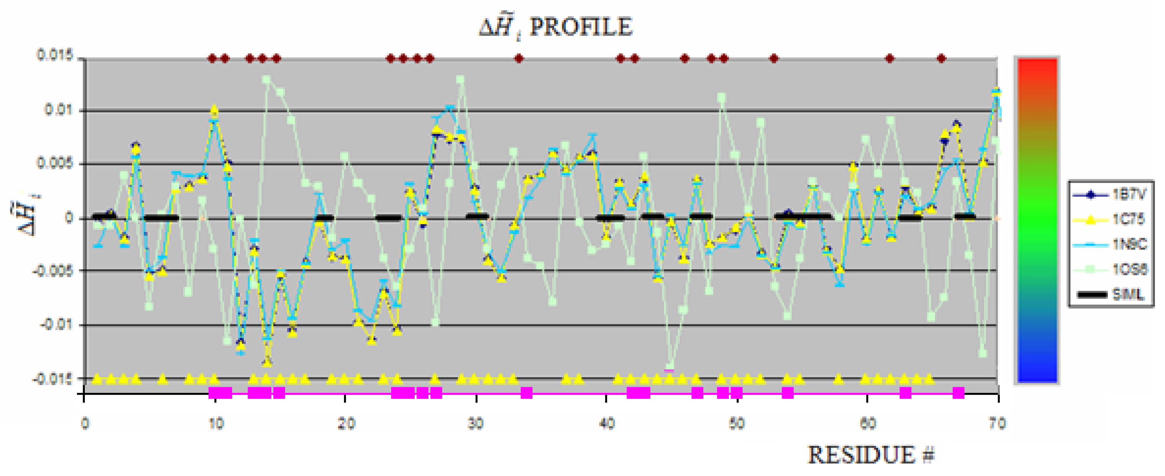
Cytochromes are characterized by hem binding. This binding in c-type cytochromes is of covalent character in contrast to the hem binding in b-type cytochromes or hemoglobin. The profiles of c-type cytochromes under consideration are shown in Figure 1.
The thick black line shows the similarity between 1OS6 and 1B7V, 1C75 (these two proteins of identical profiles) and similar one 1N9C. The yellow triangles on the X-axis show the residues engaged in ligands binding in 1OS6. The brown rectangles along the upper line (parallel to X-axis) show the residues engaged in hem binding in 1B7V, 1C75 and 1N9C. The color scale visualizes the magnitude of . This scale is applied to all figures in this paper. The pink squares identify the residues engaged in hem binding in 1B7V, 1C75 and 1N9C (Figure 1). The distribution of these residues appeared different versus those engaged in any one hem molecule in 1OS6 suggesting different mechanism leading to the structure formation in proteins under consideration. It is impossible to recognize the hem binding site on the basis of comparable analysis of profiles. However the similarity of profiles for 1B7V, 1C75 and 1N96 seems to be high. The averaged values of appeared to be quite different as shown in Table 1. expressing the low differences in profiles. The relation between hem binding site and hydrophobicity distribution is perturbed by the fact of covalent hem binding. This is why the profile in this case is not the good criteria for ligand binding site identification for “fuzzy oil drop” model.
The averaged values of being in contact with hem represent most frequently the positive value what suggests the character of hem binding site as hydrophobic deficiency cavity. The localization (as shown in Figure 1.D) seems to be similar although different residues are engaged in hem binding than in 1C75, 1B7V and 1N9C.
The structures of reduced (1N9C) and oxidized (1C75) cytochrome c553, each containing one hem molecule, appeared to be very similar. The profile similarity is accordant with structure comparison results [43]. The profile of c7-type cytochrome structure (1OS6) containing three hem molecules and additionally having bound deoxycholic acid is show in Figure 1. No similarity of characteristics for ligand binding residues can be seen. The comparison of profiles shows that the multiple ligand omplexed in c7-type cytochrome make this protein significantly changed in comparison to cytochrome c553 having one hem bound.

Table 1.
The averaged values of of residues engaged in ligand binding showing quite large differentiation of these values what excludes them to be used as ligation criterion. The values given in table are multiplied by 10*3 for simplicity.
Table 1.
The averaged values of of residues engaged in ligand binding showing quite large differentiation of these values what excludes them to be used as ligation criterion. The values given in table are multiplied by 10*3 for simplicity.
| PROTEIN | LIGAND | average Residues engaged in interaction with ligand * | average Residues not engaged in interaction with ligand* |
|---|---|---|---|
| 1B7V | Hem | 1.25 | -0.26 |
| 1C75 | Hem | 0.63 | -0.20 |
| 1N96 | Hem | 0.29 | -0.11 |
| 1OS6 | Hem1 | -3.15 | -1.22 |
| Hem2 | 1.44 | ||
| SO4 | 0.83 | ||
| DXC | 3.72 |
The 3-D representation of these proteins showing the hem binding cavity is shown in Figure 2A and 2B.
The hem binding locus can not be identified according to maxima of proteins under consideration, as it was possible in other proteins [44]. This observation is in contrast to the hem binding cavity in hemoglobin, where the residues characterized by maxima are localized in mutual close vicinity and generate the hem binding cavity [45]. The possible explanation for this observation is the different character of complexation. The hem binding in hemoglobin is based on structural and chemical compatibility stabilized by non-bonding interaction, while in c-type cytochromes the binding locus of the hem molecule is probably determined by the covalent binding making the localization of hem in a deep cavity. No ligand binding cavity can be identified in c7-type cytochrome according to its maxima localization. This suggests the conclusion that there is no common strategy for ligand (hem) binding site creation (black thick line in Figure 1). The SE parameters comparison additionally supports this observation (Table 2). The blue fragments (Figure 1) suggest that the bend fragments seem to be common for all protein belonging to this group of proteins. The analyzed proteins are a very good example to observe the influence of larger number of ligands (1OS6-A). The degree of the influence of additional ligands binding can be seen on the profile change and measured quantitatively using the SE scale.
Figure 2.
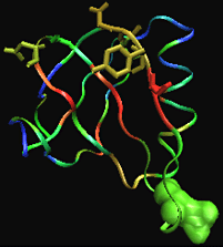
The spatial representation of 1C75 with hem bound. (a) – the ribbon representation of 1C75 colored expressing the value of . (b) – the space filling model of 1C75 showing the localization of hem in respect to the characteristics of the binding cavity. (c) – the ribbon presentation of 1N9C colored according to the scale introduced in Figure 1. ligand molecule in white (d) – the structure of 1OS6 with ligands complexed: the SO4 - yellow, DXC – white and hem – red. The color scale for ribbon as in Figure 1.
Figure 2.
The spatial representation of 1C75 with hem bound. (a) – the ribbon representation of 1C75 colored expressing the value of . (b) – the space filling model of 1C75 showing the localization of hem in respect to the characteristics of the binding cavity. (c) – the ribbon presentation of 1N9C colored according to the scale introduced in Figure 1. ligand molecule in white (d) – the structure of 1OS6 with ligands complexed: the SO4 - yellow, DXC – white and hem – red. The color scale for ribbon as in Figure 1.
The values of SE calculated for cytochromes appeared similar except the 1OS6 molecule where the binding of four ligands made the distribution of fragments of positive and negative closer to random situation (low difference of SE versus the SEmax).
2.2. Metal binding proteins
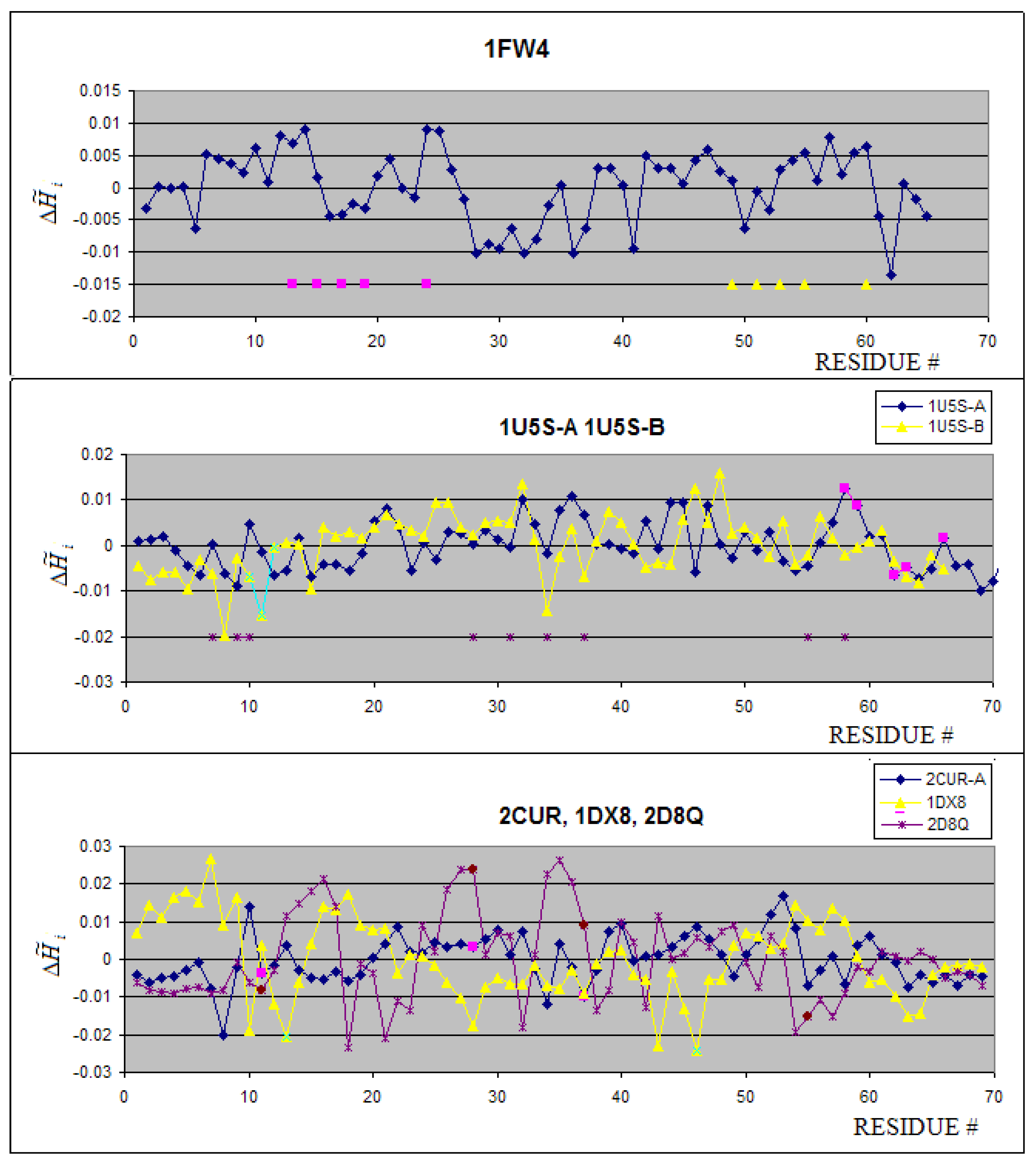
Mostly Zn(II) binding proteins are present in the group under consideration. Only calmodulin (1FW4) is complexed to Ca(II) ion. The profiles of proteins belonging to this group are shown in Figure 3A. The 3-D representation of hydrophobicity deficiency/excess is presented in Figure 4. The residues at a short distance versus the ion complexed present the values close to zero. It means that the spatial location of these residues is in agreement with the idealized hydrophobicity distribution. The profiles of 1U5S-A and 1U5S-B reveal the complexation mechanism in agreement with the FOD model (Figure 3B). The fragment of positive (local maximum) representing the hydrophobicity deficiency is complexed to the fragment of hydrophobicity excess – negative values of what makes the hydrophobicity compatibility in the contact area, although neither maximum nor minimum are of global character. The resides distinguished as pink in chain A are interacting with green fragment of chain B. The hydrophobicity compatibility of these two fragments makes the protein-protein interaction possible and stable. The brown stars near the X-axis distinguish the residues of chain A responsible for ion binding with values close to zero. The ion binding residues in 1D8Q seem to be exceptional, presenting rather contradictory values. The ion binding residues in 2CUR-A protein present close to zero values of (Figure 3C). The 1DX8 protein seems to be peculiar in that engages in ion binding residues with highly negative values (Figure 3C).
The averaged values for residues engaged in ion binding appeared to be negative (hydrophobicity excess) with the exception of the only one ion Ca2+. The Zn2+ ions are covalently bound by Cys residues, which are characterized by the highest hydrophobicity parameter (in comparison with other amino acids). Their appearance on the protein surface causes the high hydrophobicity excess on the protein surface. The Ca2+ binding cavity represents the hydrophobicity deficiency as it is observed in many cavities binding ligand [44,45].
Table 2.
The averaged values of for residues engaged in ion binding. The values given in table are multiplied by 10*3 for simplicity.
Table 2.
The averaged values of for residues engaged in ion binding. The values given in table are multiplied by 10*3 for simplicity.
| PROTEIN | ION | average Residues engaged in interaction with ion * | average Residues not engaged in interaction with ion* |
|---|---|---|---|
| FW4 | Ca2+ | 1.95 | -0.035 |
| 1U5S-B | Zn2+ | -6.40 | 0.41 |
| 2CUR | Zn2+ | -6.83 | 0.90 |
| 2D8Q | Zn2+ | -8.20 | 1.06 |
| 1DX8 | Zn2+ | -21.58 | 1.31 |
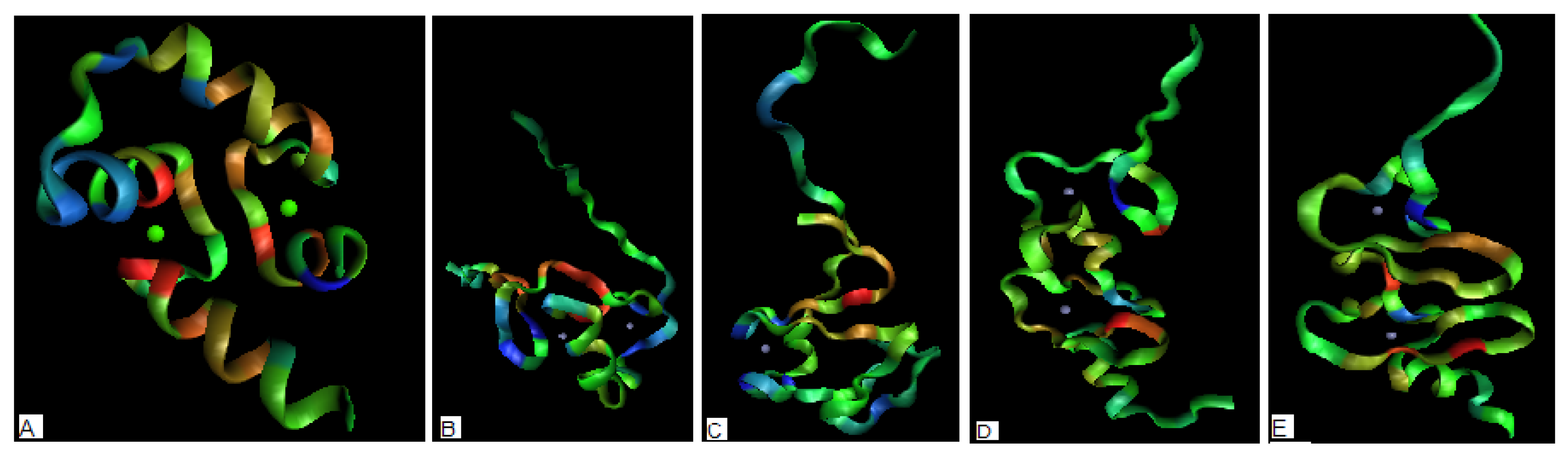
The 3-D representation of ion binding proteins visualizes the relation between ion position and the characteristics of residues responsible for ion complexation. The ion binding to proteins is electrostatic interaction oriented. This is why the localization of ions is rather difficult to be recognized according to hydrophobicity irregularity distribution. The group of ion binding proteins under consideration is quite differentiated according to SE and I parameters (Table 2, section: Metal binding). This observation is also in agreement with the profiles. The 3-D presentation with the surface characteristics reveals no specificity of residues responsible for ions binding (Figure 4) taking hydropbobicity characteristics as the criteria.
Figure 4.
The 3-D representation of the structures (the more red color – the higher hydrophobicity deficiency assumed to reveal potential ligand binding site, the more blue color – the higher hydrophobicity excess revealing potential protein-protein complexation area). The green and blue dots visualize the positions of ion(s) complexed to protein (a) – 1FW4 with two Ca(II) ions complexed (b) – 2D8Q with two Zn(II) ions complexed (c) 1DX8 with one Zn(II) ion complexed (d) – 2CUR with two Zn(II) ions complexed (e) – 1U5S-B with two Zn(II) ions complexed.

2.3. Antibiotics
The group of antibiotics is represented by Peptide
Antibiotic Bacteriotoxin AS-48 from Enterococcus faecalis. The proteins deposited in PDB as 1O82, 1O83 and 1O84 differ by the crystallization pH conditions and complexation to different molecules. The profiles of all three
proteins appeared identical (Figure 5A) (or negligibly small) what suggest negligible pH and complexation influence on the structure of the protein in this case. The 1O82-C is weakly different in
relation to the other polypeptide chains. No differences between the SE parameters have been found for these proteins (polypeptide chains). The fragments engaged in complex creation (yellow (P-P)1 and green (P-P)2 fragments
in the profile) seem to represent the complementary character of interacting surfaces (Figure 5B) (seen also in Figure 6C).
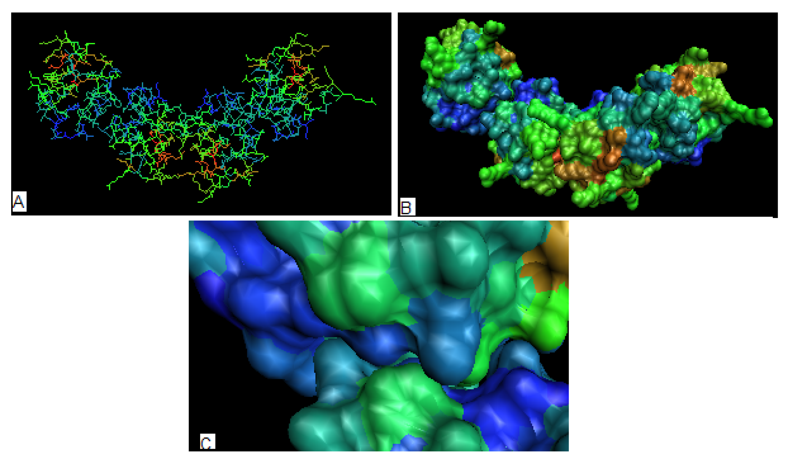
The 3-D representation of distribution in proteins engaged in the complex creation is shown in Figure 6A and 6B. The red color residues (high hydrophobicity deficiency) are almost entirely buried in the interior of the molecule, which suggests low tendency to interact with ligands as it was observed elsewhere [44,45]. The maltose bound to the protein complex interacts with residues characterized by values close to zero (Figure 5B) (hydrophilic residues) and one residue with negative (hydrophobicity excess), what may be expected taking into account the characteristics of maltose as the hydrophilic molecule as and other than hydrophobic based type of interaction is responsible for this complexation (Figure 5B). Figure 6 shows the surface characteristics and the contact areas in particular (Figure 6C) revealing the region of hydrophobicity excess on the surface being engaged in protein-protein complexation. The SE and I parameters are also identical for all the structures in this group (see Table 2, section: Antibiotics).
Figure 5.
The profiles of all chains present in 1O82, 1O83 and 1O84 (upper picture). The average value for each residue is shown in lower picture. The residues engaged in different interactions are distinguished as shown in legend.
Figure 5.
The profiles of all chains present in 1O82, 1O83 and 1O84 (upper picture). The average value for each residue is shown in lower picture. The residues engaged in different interactions are distinguished as shown in legend.
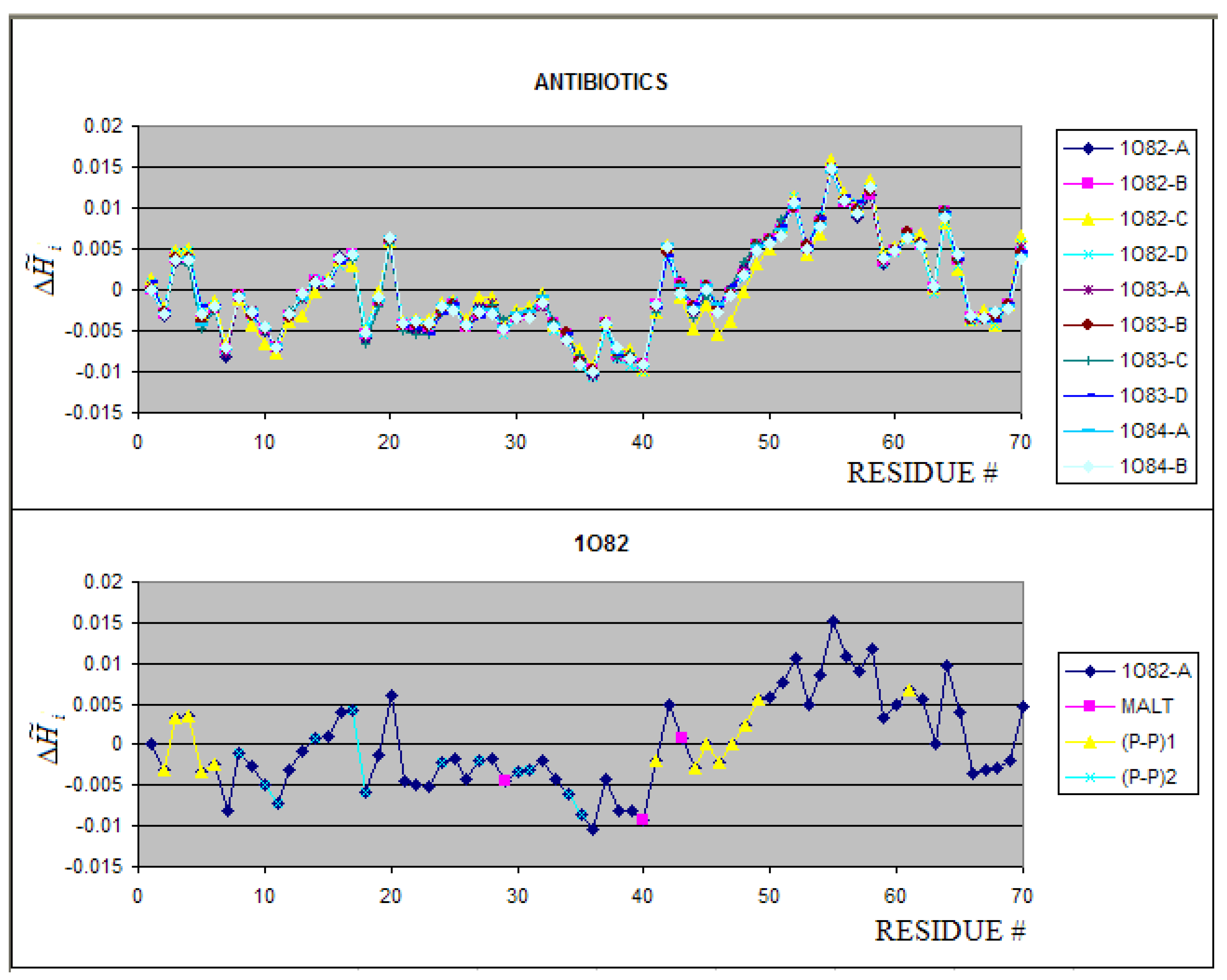
Table 3.
The averaged values calculated for residues engaged and not engaged in protein-protein complexation. The values given in table are multiplied by 10*3 for simplicity.
Table 3.
The averaged values calculated for residues engaged and not engaged in protein-protein complexation. The values given in table are multiplied by 10*3 for simplicity.
| PROTEIN | CHAIN | average Residues engaged in interaction with protein * | average Residues not engaged in interaction with protein* |
|---|---|---|---|
| 1O82 | A | -3.47 | 0.65 |
| B | -0.94 | 0.37 | |
| C | -3.33 | 0.62 | |
| D | -0.62 | 0.25 | |
| 1O83 | A | -3.40 | 0.65 |
| B | -1.20 | 0.51 | |
| C | -3.55 | 0.60 | |
| D | -0.28 | 0.11 | |
| 1O84 | A | -0.90 | 0.22 |
| B | 0.58 | -0.12 |
The values of averaged for 1O82 (1O83 and 1O84) (Table 3) calculated for residues engaged in protein-protein complexation suggest the mechanism leading to protein-protein complexation based on the hydrophobicity excess on the protein surface. The approach of residues on negative values lowers the surface of hydrophobic area in contact with water. The predictability of the protein-protein complexation seems to be possible in this case. The nonsymmetrical structure of four chains results in quite differentiated values of averaged given in Table 3.
Figure 6.
The 3-D representation of protein representing the antibiotic which is common for 1O82, 1O83 and 1O84. (a) – the distribution in a whole complex (the calculated for each unit separately) (b) – the as seen on the surface (the complex), (c) – the contact surfaces between units showing the hydrophobicity excess area being in contact.
2.4. Toxins
The group of toxin in this analysis is represented by vero-toxin, cobra-toxin, snake-toxin, scorpion-toxin and Shida-toxin. The Verotoxin is represented by the structures 1BOV and 4ULL (5 units). All units appeared to be very similar (using profiles – Figure 7, SE and I parameters (Table 2) as criteria for comparison).
The residues of negative values (hydrophobicity excess) are expected to be responsible for protein-protein complexation. It appears not to be the case in 1BOV complex. The positive values of for residues engaged in complexation suggest that other than hydrophobic interaction is the driven force for complexation.
The 3-D representation of 1BOV is shown in Figure 8. The high hydrophobicity excess areas (on surfaces – dark blue color) on the units seem to be responsible for the complex generation. The profiles of snake-toxin 1J2L-A and scorpion-toxin 1WWN-A revealing high dissimilarity are shown in Figure 7B.
The cobra-toxins are shown in Figure 9. The high similarity of the chains belonging to 2CTX as well high similarity to structures deposited as 1LXG and 1YI5 may be expressed by the profiles as well as the SE parameters.
Table 4.
The averaged values of Chains B and E were selected as the closest neighbors of chain A in seven chains symmetrical complex. *The values given in table are multiplied by 103 for simplicity.
Table 4.
The averaged values of Chains B and E were selected as the closest neighbors of chain A in seven chains symmetrical complex. *The values given in table are multiplied by 103 for simplicity.
| PROTEIN | average Residues engaged in interaction with protein* | average Residues not engaged in interaction with protein* | average Residues engaged in interaction with ligand* |
|---|---|---|---|
| 1BOV : A | 2.8 | -0.74 | |
| 1DM0 | 0.96 | -0.55 | |
| 1R4Q – B | -1.08 | 0.30 | |
| 1C48 – A | 0.70 | -0.42 | |
| 1CQF – A | 1.26 | -0.71 | |
| 1CZG – A | 1.30 | -0.85 | |
| 1CZW – A | 0.78 | -0.40 | |
| 1D1I – A | 0.55 | -1.28 | 1.71 |
| 1C4Q | 1.50 | -0.94 | |
| 1D1K | 0.65 | -0.60 | 2.15 |
| 1R4P | 0.86 | -0.57 | |
| 1YI5:F | 1.10 | -0.30 | |
| 1LXG | 6.60 | -1.20 |
Figure 8.
The 3-D representation of vero-toxin. The symmetry of the system shown in right picture. The two left pictures show the distribution of values. The helices of hydrophobicity excess character (blue color – according to the scale shown in Figure 1) seem to participate in the complex generation.

Figure 9.
The profiles for cobra-toxins. The 2CTX chains are shown in the upper picture revealing high similarity of these chains. The other proteins representing cobra-toxins in comparison with 2CTX (2CTX, 1LXG and 1YI5) are shown in lower picture.
Figure 9.
The profiles for cobra-toxins. The 2CTX chains are shown in the upper picture revealing high similarity of these chains. The other proteins representing cobra-toxins in comparison with 2CTX (2CTX, 1LXG and 1YI5) are shown in lower picture.

Figure 10.
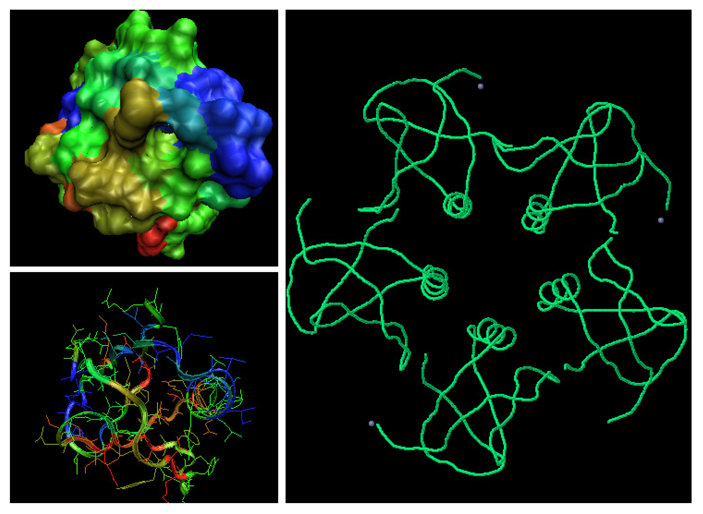
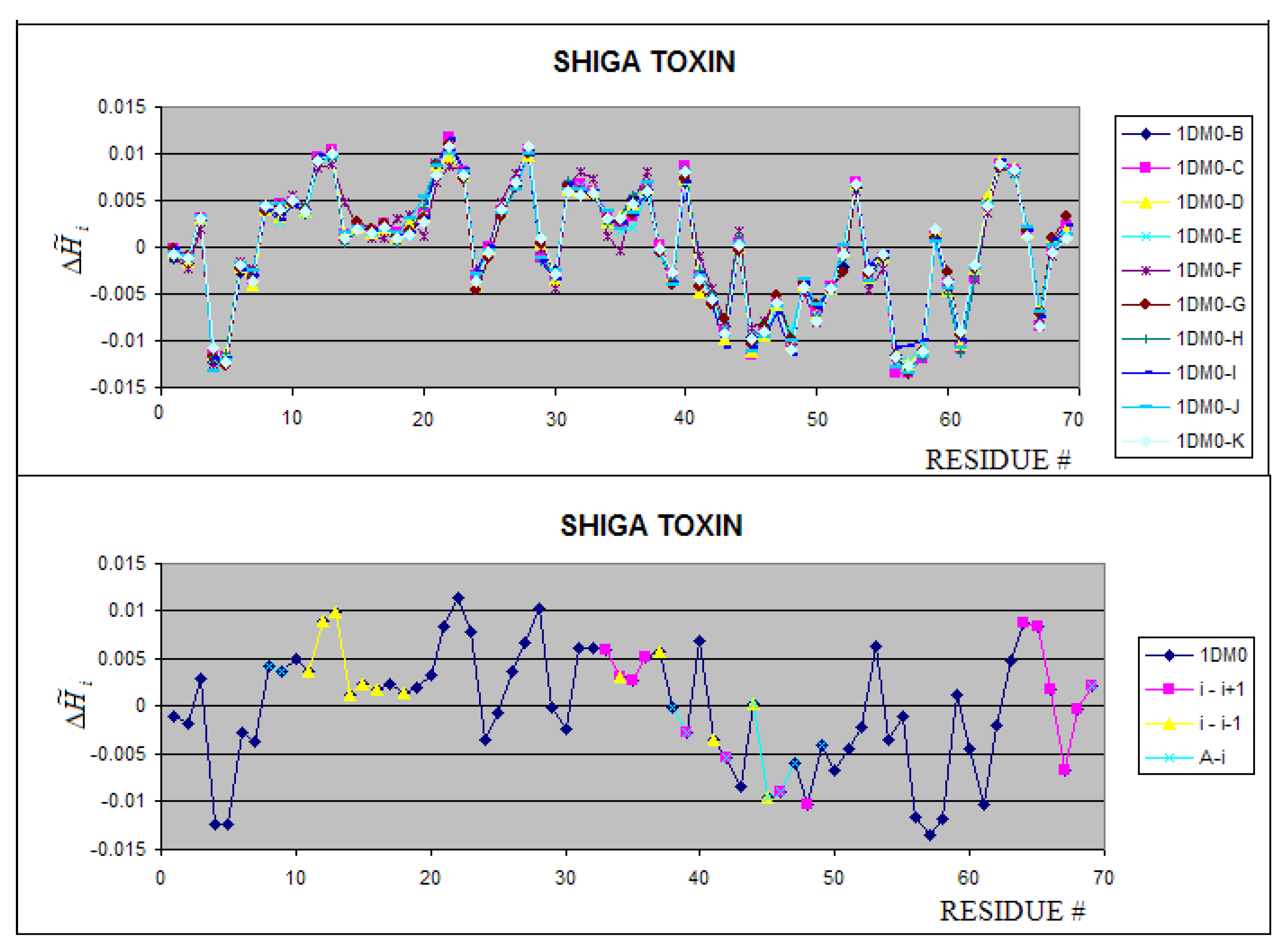
Shiga-toxins – profiles for 10 chains complexed all together revealing almost identical hydrophobicity distribution. The notation “i+1” and “i-1” denote the preceding and following neighboring molecule. The “A+i” denotes the interaction of chain “i” with chain “A” present in the complete complex not taken in the analysis (longer than 70 aa).
Figure 10.
Shiga-toxins – profiles for 10 chains complexed all together revealing almost identical hydrophobicity distribution. The notation “i+1” and “i-1” denote the preceding and following neighboring molecule. The “A+i” denotes the interaction of chain “i” with chain “A” present in the complete complex not taken in the analysis (longer than 70 aa).

Table 5.
The SE characteristics of proteins under consideration.
| Description | PDB IDa | Ligand(s)/ Othersb | SE+ | SE+max | SE+ | I+ | SE- | SE-max | SE- | I- |
| Electron transport | 1B7V:A | hem | 2.908 | 3.807 | 0.236 | 46.25 | 2.185 | 3.807 | 0.426 | 51.63 |
| 1C75:A | hem | 2.880 | 3.807 | 0.243 | 46.19 | 2.180 | 3.807 | 0.427 | 51.58 | |
| 1N9C:A | hem | 2.780 | 3.700 | 0.248 | 47.58 | 2.844 | 3.700 | 0.231 | 53.09 | |
| 1OS6:A | 3xhem, DXCc | 3.307 | 3.907 | 0.153 | 54.80 | 3.502 | 3.907 | 0.104 | 52.45 | |
| Metal binding | 1FW4:A | Ca(II) | 2.344 | 3.322 | 0.294 | 17.86 | 2.649 | 3.459 | 0.234 | 40.68 |
| 1U5S:A | - | 3.360 | 4.000 | 0.160 | 61.51 | 3.431 | 4.000 | 0.142 | 54.44 | |
| 1U5S:B | Zn(II) | 1.960 | 3.000 | 0.347 | 26.71 | 2.290 | 3.170 | 0.275 | 36.41 | |
| 2CUR:A | Zn(II) | 2.382 | 3.170 | 0.185 | 28.42 | 2.742 | 3.322 | 0.174 | 32.95 | |
| 2D8Q:A | Zn(II) | 2.437 | 3.170 | 0.231 | 23.83 | 2.605 | 3.322 | 0.216 | 27.72 | |
| 1DX8:A | Zn(II) | 1.751 | 2.585 | 0.322 | 17.47 | 2.220 | 2.585 | 0.141 | 19.10 | |
| Peptide antibiotics | 1O82:A-D | pH 4.5 | 1.229 | 3.000 | 0.590 | 23.45 | 1.666 | 2.807 | 0.406 | 28.96 |
| 1O83:A-D | pH 7.5 | |||||||||
| 1O84:A-B | MALd | |||||||||
| Toxins | 1DM0:B-K | wild type | 2.37 | 3.32 | 0.28 | 29.49 | 2.64 | 3.32 | 0.21 | 36.90 |
| 1BOV:A-E | wild type | 2.539 | 3.459 | 0.266 | 29.04 | 2.711 | 3.459 | 0.216 | 41.24 | |
| 1R4Q:B-K | wild type | 2.356 | 3.322 | 0.291 | 30.85 | 2.678 | 3.320 | 0.194 | 34.75 | |
| 4ULL | wild type | 3.268 | 3.700 | 0.117 | 55.22 | 2.389 | 3.700 | 0.354 | 43.42 | |
| 1C48:A-E | G62T | 2.711 | 3.459 | 0.262 | 35.26 | 2.720 | 3.459 | 0.213 | 34.66 | |
| 1CQF:A-E | G62T | 2.383 | 3.459 | 0.311 | 30.98 | 2.660 | 3.322 | 0.199 | 34.39 | |
| 1CZG:A-E | G62T | 2.395 | 3.170 | 0.294 | 30.28 | 2.326 | 3.170 | 0.266 | 30.93 | |
| 1CZW:A-J | W34A | 2.519 | 3.460 | 0.272 | 42.02 | 2.740 | 3.459 | 0.208 | 34.18 | |
| 1D1I:A-E | W34A | 2.520 | 3.460 | 0.272 | 42.03 | 2.741 | 3.460 | 0.208 | 34.17 | |
| 1C4Q:A-E | F30A, W34A | 2.516 | 3.459 | 0.272 | 42.06 | 2.687 | 3.459 | 0.223 | 28.71 | |
| 1D1K:A-E | D17E, W34A | 2.477 | 3.459 | 0.284 | 36.04 | 2.729 | 3.459 | 0.211 | 34.49 | |
| 1R4P:B-F | homologouse | 3.023 | 3.700 | 0.181 | 44.85 | 2.513 | 3.700 | 0.320 | 30.36 | |
| 1YI5:F-J | - | 2.393 | 3.459 | 0.308 | 24.57 | 2.663 | 3.459 | 0.230 | 41.29 | |
| 2CTX | - | 2.287 | 3.000 | 0.237 | 24.85 | 2.576 | 3.000 | 0.141 | 28.35 | |
| 1LXG:A | - | 2.331 | 3.322 | 0.298 | 37.79 | 2.510 | 3.322 | 0.244 | 35.94 | |
| 1J2L:A | - | 2.960 | 3.585 | 0.191 | 39.58 | 2.154 | 3.700 | 0.417 | 50.91 | |
| 1WWN:A | - | 3.061 | 3.907 | 0.216 | 51.20 | 3.453 | 3.907 | 0.116 | 66.87 | |
| a – additionally chain ids are given; b – pH for antibiotics or mutation variant for toxins c – deoxycholic acid d – N-decyl-_-D-maltose e – 65% sequence identity to wild type | ||||||||||
The Shiga toxin (1DM0) including 10 polypeptides of 70 amino acid residues in each unit represents a highly symmetrical system (C2 symmetry of two pentamers with C5 symmetry). The profiles for all units appeared to be identical (Figure 10). Each unit (i) interacts with two neighbors (i-1 and i+1). The fragments being in interaction contact are represented by local maxima, which interpreted as hydrophobicity deficiency. The green fragment (Figure 10 B) which is responsible for the chain A complexation seems to be stabilized mostly by hydrophobic interaction (the green fragment represents the local minimum – hydrophobicity excess).
2.5. The structural changes generated by mutation
The Shiga toxin is a good example for analysis of mutation influence on the profile (and possibly structure change due to mutation) since several mutants of this protein are present in PDB. The mutation influence can be localized using the profiles (Figure 11) and comparing the SE parameters.
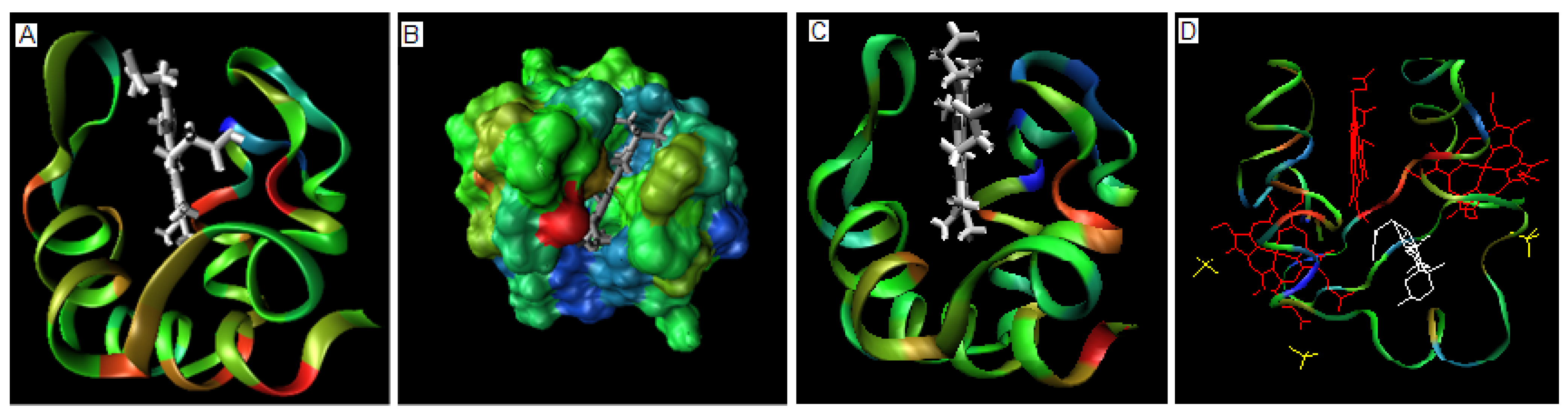
The differences between units in the 10 subunits complex of wild type (WT) Shiga toxin are negligibly small (Figure 10). The complexation in 1D1I does not reveal any structural changes versus the 1CZW which is crystallized as an individual molecule. Both molecules are W34A mutants. The consequences of mutation F30A/W34A observed in 1C4Q versus the WT molecule (1DM0) is visualized in Figure 11. The profile changes reveal the local and long range structural changes. The yellow line visualizes the magnitude of local change. The blue dots localize the mutation positions. The comparison of profiles makes possible the analysis of the structural consequences of particular mutations (Figure 12). The relation between WT and F30A/W34A as well as between F30A/W34A and W34A can be traced (see Figure 12A and 12B).
The three-dimensional Gauss function applied in FOD model was assumed to represent the distribution of hydrophobicity density in a protein molecule according to the well known model assuming that a hydrophobic center in proteins is responsible for their stability [46]. The FOD model can also be applied to simulate the external force field of hydrophobic character that directs the folding process orienting hydrophobic residues in the central part of a molecule with simultaneous exposure of hydrophilic residues on the protein surface. Application of an idealized three-dimensional Gauss function hydrophobicity distribution reveals that proteins deviate from this theoretical distribution in a specific form. The profile expressing the discrepancy between the idealized and empirical hydrophobicity distribution appeared to be specific for particular proteins characterizing their structure and function-related irregularities. The profile was used in this paper to characterize 70 amino acid residues long proteins involved in protein-ligand complexes and small protein-protein complexes. A special attention was focused on the visualization of mutant dependent structural changes. It was shown that the structural changes may have a local as well as a long range character which may be easily identified by the profiles changes and allow easy representation of these changes. The large set of mutants (including also proteins of larger size) will be presented soon. The profile will be used for the analysis of the structural and functional characteristics of NBP, the structures of which will be generated according to ROSETTA [47] and the FOD model. The comparison between the profiles of real proteins and NBP will be given.
The profile maxima representing the hydrophobicity deficiency cannot be treated as indicators for ion binding localization due to the electrostatic interaction in this case. The hem binding cavity in c-type cytochromes seems not to be hydrophobicity-based probably due to covalent binding, which determines the ligand localization.
The best applicability of FOD model seems to be the comparison of structural changes being consequence of mutation. This subject will be developed on larger group of proteins of different biological function, different size and different identified forms of biological activity failure as the consequence of mutation. The SE parameters will be used for similarity search between different groups of proteins classified according to their biological activity and in comparison with structures generated in silico according to FOD model and ROSETTA program in search for possible biological activity of NBP. The complete set of proteins of 70 amino acids in polypeptide chain is quite differentiated.
2.6. Correlation between SE and RSA (relative solvent accessibility)
Commonly used scales aimed to characterize the specificity of the protein surface like RSA (relative solvent accessibility) or ASA (accessible solvent area) are neither in correlation with nor with SE scale. Although the SE scale is aimed to characterize the participation of hydrophobicity irregularity (hydrophobicity excess and/or deficiency) versus the ideal hydrophobicity density distribution it expresses quite different issue. The SE value depends on the number of fragments representing particular characteristics and the averaged value of for each fragment. The RSA and ASA values express the global characteristics not taking under consideration the characteristics of the surface dispersion. SE values give information about the distribution and dispersion of the positive and/or negative values. This is why the correlation between them is not excluded although not expected for large number of proteins. Thus no general mutual dependency between SE and ASA or RSA is expected.
3. Conclusion
The analysis presented in this paper is aimed on estimation of the limits for “fuzzy oil drop” applicability for characteristics of structural and/or functional specificity of proteins of 70 amino acids in polypeptide chain complexed to other proteins, ligands and ions. According to the model the hydrophobicity deficiency (positive ) values is expected to bind the hydrophobic ligand (or at least its hydrophobic part). The hydrophobicity excess (negative ) when appearing on the surface points the area potentially engaged in protein-protein complexation. As shown in this paper it was found for selected proteins (antibiotics and partially for toxins). The protein-protein complexation appeared possible as results of the interaction of fragments of positive generating the complex according to the mechanism as predicted for protein-ligand complexation mechanism. It seems to be also accordant to the model making two partners of complexation engaged in complementary irregularity accomplishment.
The SE scale was introduced to measure the degree of structural and/or functional similarity. The comparison of large number of SE values calculated for different proteins allows the search for similarity. It is of special importance in case of proteins of unknown biological function, the number of which is permanently growing in PDB [48].
The applicability of the “fuzzy oil drop” based model profiles changed being the result of structural changes on mutation seems to be quite useful. Both the profiles and Se scale seem to express the mutation influence in qualitative and quantitative form. This applicability of “fuzzy oil drop” model will be analyzed for larger group pf proteins to verify this observation.
4. Data and Methods
4.1. Data
The tool available on PDB webpage oriented on the search for proteins satisfying particular conditions was used to extract the proteins according to a defined polypeptide chain length. The proteins containing 70 amino acid residues were selected. However some examples of proteins of chain length between 68 and 72 amino acids were also taken under consideration. The proteins
Table 6.
Proteins and their short characteristics taken for analysis.
| Description | Protein name | Source Organism | PDB entries a |
| Electron transport | cytochrome c553 | Bacillus pasteurii | 1B7V, 1C75, 1N9C |
| cytochrome c7 | Geobacter sulfurreducens | 1OS6 | |
| Metal binding | calmodulin | Bos taurus | 1FW4 |
| cytoplasmic protein NCK2 | Homo sapiens | 1U5S | |
| Skeletal muscle LIM-protein 1 | Homo sapiens | 2CUR | |
| BLu protein | Homo sapiens | 2D8Q | |
| rubredoxin | Homo sapiens | 1DX8 | |
| Peptide antibiotic | AS-48 protein | Enterococcus faecalis | 1O82, 1O83, 1O84 |
| Toxin | Shiga toxin subunit B | Shigella dysenteriae | 1DM0*, 1R4Q* |
| Escherichia coli | 1CQF*, 1D1I* | ||
| Bacteriophage H30 | 1CZG*, 1CZW* | ||
| Shiga-like toxin 1 subunit B | Escherichia coli | 1BOV, 1D1K*, 1C4Q* | |
| Bacteriophage H30 | 1C48*, 4ULL* | ||
| Shiga-like toxin 2 subunit B | Escherichia coli | 1R4P* | |
| Alpha-cobratoxin | Naja kaouthia | 1LXG* | |
| Naja naja | 2CTX* | ||
| Naja siamensis | 1YI5* | ||
| BmKIT1 | Mesobuthus martensii | 1WWN* | |
| disintegrin triflavin | Trimeresurus flavoviridis | 1J2L* |
a – PDB entries containing protein-protein complexes are denoted by *.presented in this paper belong to different groups (according to the biological function): electron transfer, metal binding proteins, antibiotic, and toxins (see Table 2). The toxins present in the data base are of particular interest due to the availability of few mutant forms, which are characterized with respect to structural changes classified according to the FOD model.
4.2. The protein-ligand contacts analysis
The search for residues being in a close distance (interaction distance) with the ligand molecule or another protein molecule (in protein-protein complexes) has been made using the PDBsum database (www.ebi.ac.uk/pdbsum/) [49].
4.3. The structural/functional characteristics
The basis of FOD model applied for the identification of hydrophobicity deficiency/excess in protein molecules, which appeared to be strongly structure (and function) dependent is very simple. The value of the difference between theoretically assumed hydrophobicity () distribution in a protein (which is assumed to be represented by a three-dimensional Gauss function) and that empirically observed () described according to Levitt [50] function, defines hydrophobicity irregularity:
where:
The values with index “sum” express the total value of appropriate hydrophobicity to make the theoretical and empirical distribution normalized, making possible comparison of these values. The symbols denote the hydrophobicity parameter describing each amino acid [51] or any other hydrophobicity scale can be applied). The values with indexes i, j describe the points representing individual residues (amino acid residue geometric center).
The eq.2. expresses the three-dimensional Gauss function. The value of this function is interpreted as hydrophobicity density in idealized case. The Gauss function maximum localized in the point expresses the highest hydrophobicity density localized in the center of the ellipsoid. The Gauss function values decrease according to exponential function reaching values close to zero in a certain distance versus the center. This distance changes depending on the values of (standard deviations), which can be different for different axes.
The eq.3. expresses the method to calculated the empirical hydrophobicity density distribution being the result of the specific localization of residues representing specific hydrophobicity parameters. The values represent the hydrophobicity collecting all hydrophobic interactions in distance below cut off (15Å). The normalization of both function values (division by the sum of all i-th values) makes possible calculation of the differences between theoretical idealized hydrophobicity density distribution and the observed one in particular protein (eq.1.). This is why the profile expresses the irregularity producing the maxima for hydrophobicity deficiency and minima for hydrophobicity excess.
profile reveals the areas in a protein molecule which seem to be of a specific character describing the structure and related to biological function. The profile shows the fragments of hydrophobicity deficiency ( > 0) and hydrophobicity excess ( < 0). The distribution and the length of fragments of positive and negative can be interpreted on the basis of information theory assuming that the generation of structures with residues characterized by positive localized in close mutual vicinity is a non-random event. The information entropy (according to Shannon definition [52]) is expressed as:
Where pj expresses the sum of values for j-th
fragment (all consecutive >
0) divided by sum of all positive values.
SE depends on the number of K-fragments and their pi mutual relation, and therefore maximum (SEmax) for particular K elements (fragments) when all probabilities (pi) are equal, representing the random solution exists. The larger is the difference between SEmax and SE denoted by ΔSE, the less random character represents the localization of residues with positive . The closer to SEmax is the calculated
value of SE the more random is the process producing a particular profile. SE
can be calculated for fragments of positive (hydrophobicity deficiency) as well as for fragments of negative (hydrophobicity excess). This is a way to compare proteins and in consequence to measure their mutual similarity. The profiles and SE calculations will be used for protein structures description. The color scale shown in figures representing the profiles is also applied also for 3-D representation of proteins, showing the distribution of hydrophobicity deficiency/excess. Similar (or identical) profile and/or similar or identical SE parameters may suggest a structural and/or functional similarity. The FOD model as well as SE calculation was applied to evaluate the structural and/or functional differentiation in the group of proteins listed in the Table 1.
Following quantity used in the study of binding sites is the information (I) necessary to localize residues creating the binding site (presence of any form of disorder may be interpreted as potential localization for any form of interaction). The participation of particular residues in the potential active site creation is understood as a probability expressing conjunction of events (close mutual localization) and can be created according to equation:
where K and pj have the same meaning as in the equation (4).
4.4. Relative solvent accessibility
The relation between solvent and protein molecule was measured using standard models implemented in the program ASA-View (http://www.netasa.org/asaview/). This application allows calculation of ASA (accessible surface area) and recalculates to the RSA scale. Additionally the DSSP program was applied in the calculation procedure [53].
The calculation was performed to search for correlation of SE scale with other methods oriented on protein-solvent relation.
Acknowledgments
The Authors are very grateful to prof Leszek Konieczny (Institute of Medical Biochemistry, Collegium Medicum, Jagiellonian University, Krakow, Poland) for fruitful discussion. This research was supported Collegium Medicum grants 501/P/266/L. This work has been funded by the European Commission EUChinaGRID project (contract number: 026634).
References
- Ladner, R.C. Constrained peptides as binding entities. Trends Biotechnol 1995, 13, 426–430. [Google Scholar] [CrossRef] [PubMed]
- Ladner, R.C. Phage display and pharmacogenomics. Pharmacogenomics 2000, 1, 99–202. [Google Scholar] [CrossRef]
- Neri, D.; Petrul, H.; Roncucci, G. Engineering recombinant antibodies for immunotherapy. Cell Biophys 1995, 27, 47–61. [Google Scholar] [CrossRef] [PubMed]
- Siegel, D.L. Research and clinical applications of antibody phage display in transfusion medicine. Transfus Med. Rev. 2001, 15, 35–52. [Google Scholar] [CrossRef] [PubMed]
- Griffiths, A.D. Production of human antibodies using bacteriophage. Curr. Opin. Immunol 1993, 5, 263–267. [Google Scholar] [CrossRef]
- Winter, G.; Grifiths, A.D.; Hawkins, R.E.; Hoogenboom, H.R. Making antibodies by phage display technology. Annu Rev Immunol 1994, 12, 433–455. [Google Scholar] [CrossRef] [PubMed]
- Hoogenboom, H.R.; de Bruïne, A.P.; Hufton, S.E.; Hoet, R.M.; Arends, J.W.; Roovers, R.C. Antibody phage display technology and its applications. Immunotechnology 1998, 4, 1–20. [Google Scholar] [CrossRef] [PubMed]
- Frauenfelder, H.; Wolynes, P.G. Biomolecules: Where the physics of complexity and simplicity meet. Phys. Today 1994, 47, 58–64. [Google Scholar] [CrossRef]
- Chan, H.S. Dill, K.A. The protein folding problem. Phys. Today 1993, 46, 24–42. [Google Scholar] [CrossRef]
- Karplus, M.; Shakhnovich, E.I. Protein Folding. W. H. Freeman & Co.: New York, 1992. [Google Scholar]
- Covell, D.G.; Jernigan, R.L. Conformations of folded proteins in restricted spaces. Biochemistry 1990, 29, 3287–3294. [Google Scholar] [CrossRef]
- Shakhnovich, E.I.; Gutin, A.M. Implications of thermodynamics of protein folding for evolution of primary sequences. Nature 1990, 346, 773–775. [Google Scholar] [CrossRef] [PubMed]
- Skolnick, J.; Kolinski, A. Simulations of the folding of a globular protein. Science 1990, 250, 1121–1125. [Google Scholar] [CrossRef] [PubMed]
- Lau, K.F.; Dill, K.A. A lattice statistical mechanics model of conformational and sequence spaces of proteins. Macromolecules 1989, 22, 3986–3997. [Google Scholar] [CrossRef]
- Taketomi, H.; Ueda, Y.; Gofi, N. Studies on protein folding, unfolding and fluctuations by computer simulation. I. The effect of specific amino acid sequence represented by specific inter-unit interactions. Int J Pept Protein Res 1975, 7, 445–459. [Google Scholar] [CrossRef] [PubMed]
- Rode, B.M. Peptides and the origin of life. Peptides 1999, 20, 773–786. [Google Scholar] [CrossRef]
- Orgel, L.E. The origin of life - how long did it take? Orig Life Evol Biosph 1998, 28, 91–96. [Google Scholar] [CrossRef]
- Schwartz, A.W. The Molecular Origins of Life: Assembling Pieces of the Puzzle. Cambridge University Press: Cambridge, 1998. [Google Scholar]
- Ferris, J.P.; Hill, A.R.; Liu, R.; Orgel, L.E. Synthesis of long prebiotic oligomers on mineral surfaces. Nature 1996, 381, 59–61. [Google Scholar] [CrossRef]
- Radzicka, A.; Wolfenden, R. Rates of uncatalyzed peptide bond hydrolysis in neutral solution and the transition state a_nities of proteases. Journal of the American Chemical Society 1996, 118, 6105–6109. [Google Scholar] [CrossRef]
- Luisi, P.L. The Emergence of Life. From Chemical Origins to Synthetic Biology. Cambridge University Press: London, 2006. [Google Scholar]
- Lingen, B.; Grötzinger, J.; Kolter, D.; Kula, M.R.; Pohl, M. Improving the carboligase activity of benzoylformate decarboxylase from Pseudomonas putida by a combination of directed evolution and site-directed mutagenesis. Protein Eng 2002, 15, 585–593. [Google Scholar] [CrossRef]
- Meyer, A.; Schmid, A.; Held, M.; Westphal, A.H.; Rothlisberger, M.; Kohler, H.P.E.; van Berkel, W.J.H.; Witholt, B. Changing the substrate reactivity of 2-hydroxybiphenyl 3-monooxygenase from pseudomonas azelaica hbp1 by directed evolution. J Biol Chem 2002, 277, 5575–5582. [Google Scholar] [CrossRef]
- Otten, L.G.; Sio, C.F.; Vrielink, J.; Cool, R.H.; Quax, W.J. Altering the substrate specificity of cephalosporin acylase by directed evolution of the beta-subunit. J Biol Chem 2002, 277, 42121–42127. [Google Scholar] [CrossRef] [PubMed]
- Matsumura, I.; Ellington, A.D. In vitro evolution of beta-glucuronidase into a beta-galactosidase proceeds through non-specific intermediates. J Mol Biol 2001, 305, 331–339. [Google Scholar] [CrossRef] [PubMed]
- Persson, E.; Kjalke, M.; Olsen, O.H. Rational design of coagulation factor via variants with substantially increased intrinsic activity. Proc Natl Acad Sci U S A 2001, 98, 3583–13588. [Google Scholar] [CrossRef] [PubMed]
- Rellos, P.; Ma, J.; Scopes, R.K. Alteration of substrate specificity of zymomonas mobilis alcohol dehydrogenase-2 using in vitro random mutagenesis. Protein Expr Purif 1997, 9, 83–90. [Google Scholar] [CrossRef]
- Neylon, C. Chemical and biochemical strategies for the randomization of protein encoding dna sequences: library construction methods for directed evolution. Nucleic Acids Res 2004, 32, 1448–1459. [Google Scholar] [CrossRef]
- Cirino, P.C.; Mayer, K. M.; Umeno, D. Generating mutant libraries using error-prone PCR. Methods Mol Biol 2003, 231, 3–9. [Google Scholar]
- Murakami, H.; Hohsaka, T.; Sisido, M. . Random insertion and deletion of arbitrary number of bases for codon-based random mutation of DNA’s. Nat Biotechnol 2002, 20, 76–81. [Google Scholar] [CrossRef]
- Murakami, H.; Hohsaka, T.; Sisido, M. Random insertion and deletion mutagenesis. Methods Mol Biol 2003, 231, 53–64. [Google Scholar]
- Shao, Z.; Zhao, H.; Giver, L.; Arnold, F.H. Random-priming in vitro recombination: an effective tool for directed evolution. Nucleic Acids Res 1998, 26, 681–683. [Google Scholar] [CrossRef]
- Cadwell, R.C.; Joyce, G.F. Mutagenic pcr. PCR Methods Appl 1994, 3, S136–S140. [Google Scholar] [CrossRef]
- Aguinaldo, A.M.; Arnold, F.H. Staggered extension process (step) in vitro recombination. Methods Mol Biol 2003, 231, 105–110. [Google Scholar]
- Coco, W.M. RACHITT: Gene family shuffling by Random Chimera genesis on Transient Templates. Methods Mol Biol 2003, 231, 111–127. [Google Scholar] [PubMed]
- Lutz, S.; Ostermeier, M. Preparation of scratchy hybrid protein libraries: size- and in-frame selection of nucleic acid sequences. Methods Mol Biol 2003, 231, 143–151. [Google Scholar] [PubMed]
- Ostermeier, M.; Lutz, S. The creation of ITCHY hybrid protein libraries. Methods Mol Biol 2003, 231, 129–141. [Google Scholar]
- O'Maille, P.E.; Bakhtina, M.; Tsai, M.D. Structure-based combinatorial protein engineering (scope). J Mol Biol 2002, 321, 677–691. [Google Scholar] [CrossRef]
- Joern, J.M. DNA shuffing. Methods Mol Biol 2003, 231, 85–89. [Google Scholar] [PubMed]
- Chiarabelli, C.; Vrijbloed, J.W.; Lucrezia, D.D.; Thomas, R.M.; Stano, P.; Polticelli, F.; Ottone, T.; Papa, E.; Luisi, P.L. Investigation of de novo totally random biosequences, Part II: On the folding frequency in a totally random library of de novo proteins obtained by phage display. Chem Biodivers 2006, 3, 840–859. [Google Scholar] [CrossRef]
- Chiarabelli, C.; Vrijbloed, J.W.; Thomas, R.M.; Luisi, P.L. Investigation of de novo totally random biosequences, Part I: A general method for in vitro selection of folded domains from a random polypeptide library displayed on phage. Chem Biodivers 2006, 3, 827–839. [Google Scholar] [CrossRef]
- Berman, H.M.; Battistuz., T.; Bhat, T.N.; Bluhm, W.F.; Bourne, P.E.; Burkhardt, K.; Feng, Z.; Gilliland, G.L.; Iype, L.; Jain, S.; Fagan, P.; Marvin, J.; Padilla, D.; Ravichandran, V.; Schneider, B.; Thanki, N.; Weissig, H. Westbrook JD, Zardecki C. The Protein Data Bank. Acta Crystallogr D Biol Crystallogr 2002, 58, 899–907. [Google Scholar] [CrossRef]
- Bartalesi, I.; Bertini, I.; Rosato, A. Structure and dynamics of reduced bacillus pasteurii cytochrome c: oxidation state dependent properties and implications for electron transfer processes. Biochemistry 2003, 42, 739–745. [Google Scholar] [CrossRef]
- Brylinski, M.; Konieczny, L.; Roterman, I. Ligation site in proteins recognized in silico. Bioinformation 2006, 1, 127–129. [Google Scholar] [CrossRef] [PubMed]
- Brylinski, M.; Konieczny, L.; Roterman, I. Is the protein folding an aim-oriented process? Human haemoglobin as example. Int J Bioinform Res Appl 2007, 3, 234–260. [Google Scholar] [CrossRef]
- Kauzmann, W. Some factors in the interpretation of protein denaturation. Adv Protein Chem 1959, 14, 1–63. [Google Scholar] [PubMed]
- Simons, K.T.; Ruczinski, I.; Kooperberg, C.; Fox, B.A.; Bystroff, C.; Baker, D. Improved recognition of native-like protein structures using a combination of sequence-dependent and sequence-independent features of proteins. Proteins 1999, 34, 82–95. [Google Scholar] [CrossRef]
- Prymula, K.; Roterman, I. Functional Characteristics of Small Proteins (70 amino acid residues) Forming Protein-Nucleic Acid Complexes. J. Biomol. Struct Dynam. – in press. [CrossRef]
- Laskowski, R.A.; Chistyakov, V.V. Thornton JM. PDBsum more: new summaries and analyses of the known 3d structures of proteins and nucleic acids. Nucleic Acids Res 2005, 33, D266–D268. [Google Scholar] [CrossRef]
- Levitt, M. A simplified representation of protein conformations for rapid simulation of protein folding. J Mol Biol 1976, 104, 59–107. [Google Scholar] [CrossRef]
- Kyte, J.; Doolittle, R.F. A simple method for displaying the hydropathic character of a protein. J Mol Biol 1982, 157, 105–132. [Google Scholar] [CrossRef]
- Shannon, C. A mathematical theory of communication. The Bell System Technical Journal 1948, 27, 379–423, 623–656. [Google Scholar] [CrossRef]
- Ahmad, S.; Gromiha, M.M.; Fawareh, H.; Sarai, A. ASAView: Solvent Accessibility Graphics for proteins. BMC Bioinformatics 2004, 5, 51. [Google Scholar] [CrossRef]
Figure 1.
The profiles for proteins belonging to the group of cytochromes.

Figure 3.
The profiles of proteins complexed with metal ions. (a) – the pink symbols denote the Ca(II) binding residues, the yellow triangles show the residues engaged in the second Ca(II) ion. (b) – the brown stars denote the residues in chain A engaged in Zn(II) binding, pink residues in chain A are engaged in complex creation with residues distinguished as yellow triangles in chain B, (c) pink symbols distinguish the resides in 2CUR-A engaged in Zn(II) binding, brown symbols distinguish the residues binding Zn(II) in 2D8Q, and green stars distinguish residues engaged in Zn(II) ion binding in DX8.

Figure 7.
The profiles of 1BOV and 4ULL (upper picture) and other toxins (1WWN – scorpio-toxin and 1J2L-A -snake toxin) (lower picture).
Figure 7.
The profiles of 1BOV and 4ULL (upper picture) and other toxins (1WWN – scorpio-toxin and 1J2L-A -snake toxin) (lower picture).
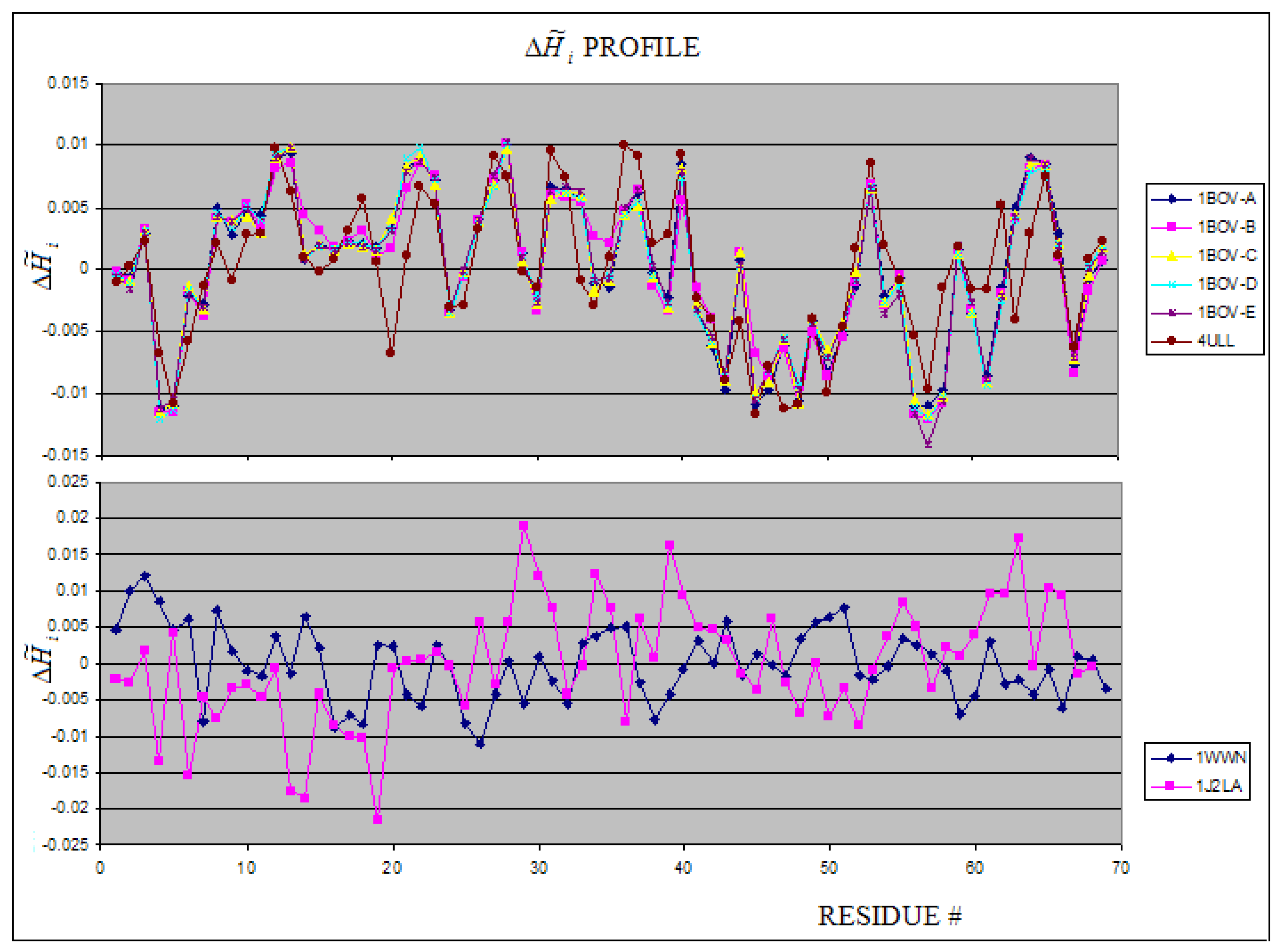
Figure 11.
Influence of mutation on the profiles. The blue dots position the residue mutated. The profile shows the close neighborhood as well as long range influence of mutation on the structural and possibly functional form.
Figure 11.
Influence of mutation on the profiles. The blue dots position the residue mutated. The profile shows the close neighborhood as well as long range influence of mutation on the structural and possibly functional form.
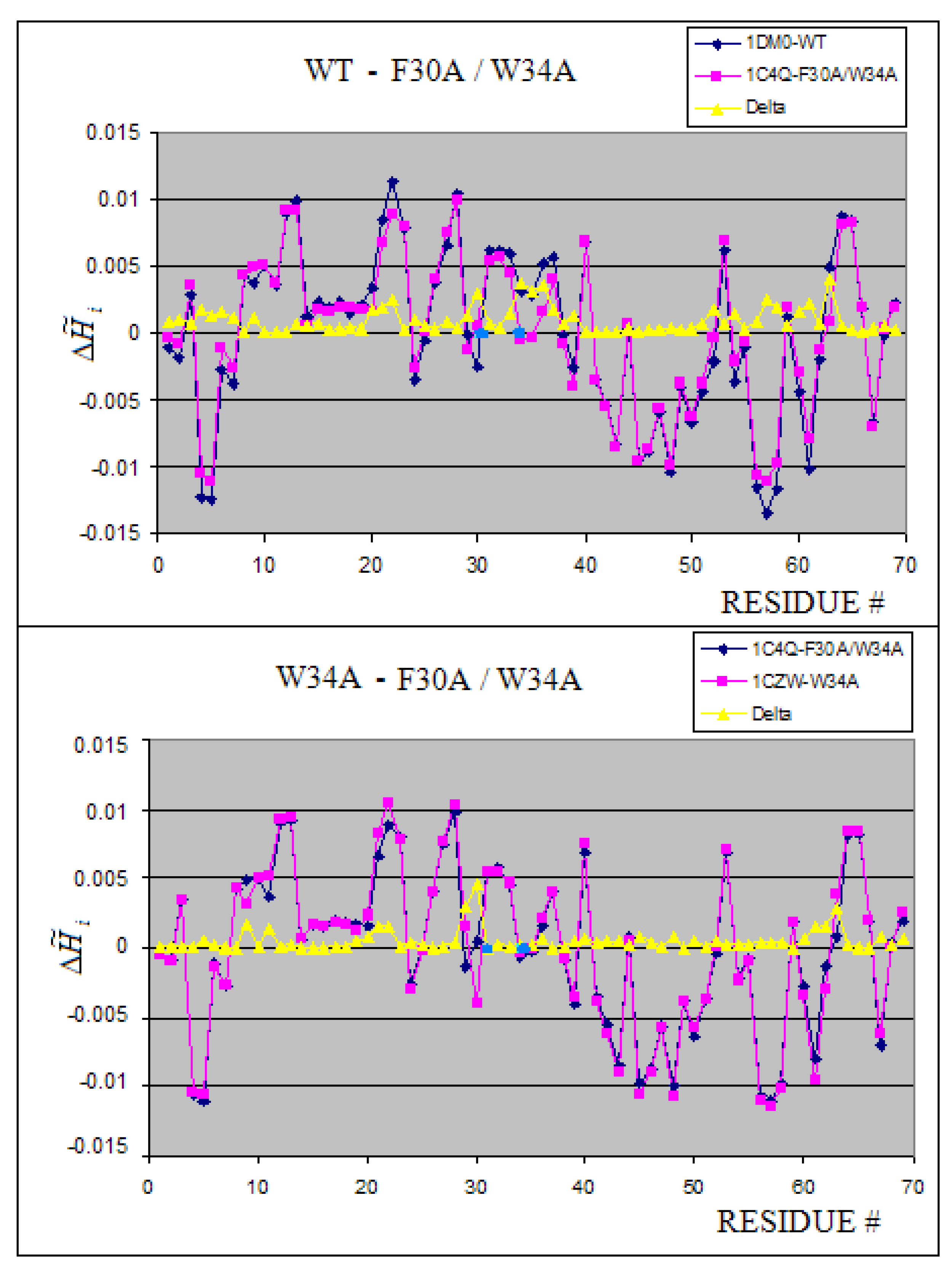
Figure 12.
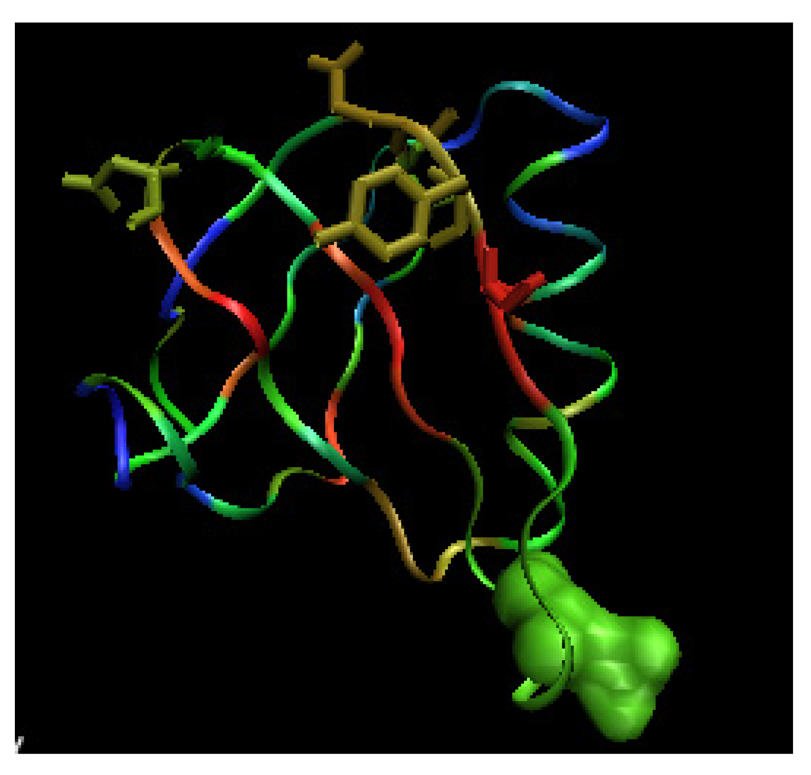
3-D representation of Shiga-toxin (wild type). The color scale denotes the magnitude of . The space filling representation – the mutated residue, the side chains in sticks representation – the residues influences by the mutation recognized according to the profile.
Figure 12.
3-D representation of Shiga-toxin (wild type). The color scale denotes the magnitude of . The space filling representation – the mutated residue, the side chains in sticks representation – the residues influences by the mutation recognized according to the profile.

Publisher’s Note: MDPI stays neutral with regard to jurisdictional claims in published maps and institutional affiliations. |
© 2009 by the authors. Licensee MDPI, Basel, Switzerland. This article is an open access article distributed under the terms and conditions of the Creative Commons Attribution (CC BY) license (https://creativecommons.org/licenses/by/4.0/).
Share and Cite
MDPI and ACS Style
Prymula, K.; Roterman, I. Structural Entropy to Characterize Small Proteins (70 aa) and Their Interactions. Entropy 2009, 11, 62-84. https://doi.org/10.3390/e11010062
AMA Style
Prymula K, Roterman I. Structural Entropy to Characterize Small Proteins (70 aa) and Their Interactions. Entropy. 2009; 11(1):62-84. https://doi.org/10.3390/e11010062
Chicago/Turabian StylePrymula, Katarzyna, and Irena Roterman. 2009. "Structural Entropy to Characterize Small Proteins (70 aa) and Their Interactions" Entropy 11, no. 1: 62-84. https://doi.org/10.3390/e11010062