The Influence of Shape on Parallel Self-Assembly

Abstract

Self-assembly is a key phenomenon whereby vast numbers of individual components passively interact and form organized structures, as can be seen, for example, in the morphogenesis of a virus. Generally speaking, the process can be viewed as a spatial placement of attractive and repulsive components. In this paper, we report on an investigation of how morphology, i.e., the shape of components, affects a self-assembly process. The experiments were conducted with 3 differently shaped floating tiles equipped with magnets in an agitated water tank. We propose a novel measure involving clustering coefficients, which qualifies the degree of parallelism of the assembly process. The results showed that the assembly processes were affected by the aggregation sequence in their early stages, where shape induces different behaviors and thus results in variations in aggregation speeds.

1. Introduction

Inspection of the microscopic world of living systems often confronts us with the core mystery of its amazing capability. In particular, self-assembly is considered to be one of the principal aspects that one observes in living systems, on the micro-scale [1]. Some fundamental phenomena, such as the morphogenesis of viruses, offer a key to an understanding of the central issues of “living” systems. Knowledge from molecular biology reminds us of the importance of the fertile encoding capability of molecular bonding; it is noteworthy that no matter how complicated the microscopic systems seem, they exploit non-covalent bonds (hydrogen bonds, ionic bonds, and van der Waals attractions) as interaction forces and somehow achieve an amazing specificity in docking with other selected molecules. Considering the fact that molecules exploit the bonding affinity level for maintaining connections, this encoding power is noteworthy. The trick of distributing bonding sites around the body, and having flexible switches to change the morphology are considered to be hidden in the shape and the dynamics [2,3]. It is therefore necessary to take stochasticity and morphology into account when studying these issues.

In contrast to the variety of sets of compounds so far revealed, however, discussions of the emergence of life from local interactions of components still gravitate around in-depth descriptions and modeling of interactions, e.g., through steady-state representations such as reaction pathways. The intricate web of reaction networks provides us with the requisite level of complexity, and the global picture suggests to us the importance of understanding the dynamics from the perspective of distributed systems [4]. Understanding of the main global features of the dynamics of self-assembly has not yet been achieved. As the metaphor the mechanism of a single cell is more complex than a Boeing 777 implies, it is necessary to tackle the issue from another direction—the so called synthetic approach. Efforts are required to abstract higher level design principles to clarify the actual dynamic processes underlying these interactions.

There have been numerous attempts undertaken in various fields. A pioneering approach was taken by Penrose about 50 years ago [5]. He developed a mechanical self-replication model, which operated in a stochastic manner. Aggregation patterns of passive self-assembly were raised into prominence and employed by Hosokawa et al. [6,7]. He examined the effect of active elements on the aggregation. Whitesides and his group investigated many self-assembling and self-organizing phenomena at different scales [8,9,10,11] and categorized them into static, dynamic, templated, and biological self-assemblies, depending on the energy dissipation. Seminal ideas about conformational switching were proposed by Saitou [12]. He proposed a reactive mechanism for 1D self-assembly and assessed the functionality with kinetic rate equations. The units he designed feature mechanical internal states, such that the units react differently to their inputs, whereas the system is purely passive with respect to physical causation.

By mimicking tools and methods from nature, many advances have been made in utilizing self-assembly for the fabrication of structures at molecular scales [13,14,15,16,17,18]. An important fact to stress here is that the models are grounded in real entities; thus they provide us with effective ideas. Also, the capacity level of the number of components that can be treated in each experiment is a certain advantage. Concerns that we have to confront include the difficulty of controllability, that is, the lack of a capability to directly adjust the level of activity.

To date, few stochastic self-assembling robots have been developed in the field of modular robotics (White et al. [19,20]; Shimizu et al. [21]; Bishop et al. [22]; Griffith et al. [23]; Nagy et al. [24]; Miyashita et al. [25,26]). In contrast to the advantage of such an approach—the possibility of its controllability—technological constraints such as heavy and big motors or large power consumption prevent the systems from being highly functional. Also, a certain amount of state-based control is required for the assembly process, which results in systems less suited to their complex environments.

In this paper, we use a simple yet effective model for the analysis of self-assembly—tiles with magnets in a stochastic environment—and examine the aggregation patterns as a function of the shapes of tiles. We characterize the diverse figures of molecules by the combination of shapes and magnetic forces. Besides we introduce a novel notion, the Degree of parallelism (DOP) as a measure of self-assembly and experimentally confirm its validity.

The paper is organized as follows. In Section 2, we describe the tiles and the experimental setup. Then, in Section 3, we describe the interaction mechanism, in particular the magnetic interaction, and introduce measures to quantify the self-assembly process. In Section 4, we present experimental results and a detailed analysis. This is followed by a discussion in Section 5 and Section 6 concludes the paper.

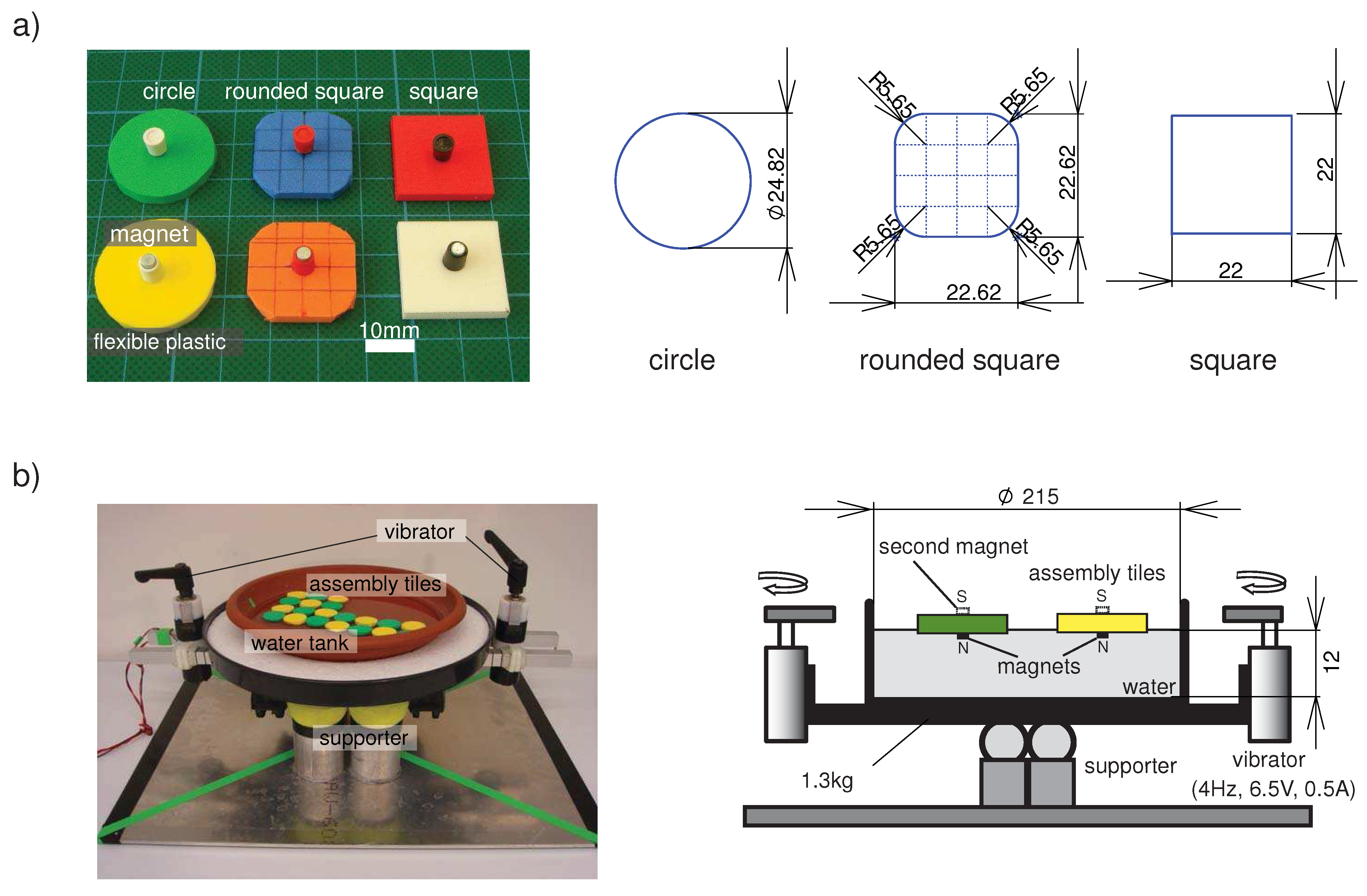
2. The Experimental Self-Assembly Platform

In order to evaluate the role of morphology in the self-assembly process, we constructed an experimental platform, which consisted of floating tiles equipped with magnets, and a water tank with two vibrators (4 Hz, 6.5 V, 0.5 A) that induced turbulence on the water surface and thus provided randomness (Figure 1 b, total weight:1.3kg). We developed tiles with three different shapes (Figure 1 a): circles, squares, and squares with rounded corners. They were of identical weight (0.2 g), surface area (484 mm${}^2$) and thickness (2 mm). These shapes were selected after noting that a change in one variable coding the morphology, e.g., surface area, tended to affect the other dependent variables, e.g., diameter, shortest distance between edges and magnets.

On each tile, one or two (for the double magnet type) vertically oriented magnets were attached. The double magnet type was constructed to investigate the effects of magnetic strength (as depicted in Figure 1 b right, “second magnet”). On the water, a floating tile whose magnet pointed upwards attracted the other type whose magnet pointed downwards, whereas tiles with the same type of magnets repelled each other. Colors were introduced to distinguish between attracting and repelling tiles and to facilitate visual inspection of the self-assembly progress. For example, the magnet on the green circular tile in Figure 1 a is oriented opposed to the magnet on the yellow circular tile. Exploiting these characteristics, we examined how such multiple tiles formed a structure through the interactions. For each trial, we initialized the positions of the tiles. Using a spacer, 10 tiles of the same color were placed in one side of the tank, and 10 tiles of the other color were placed at the opposite side. Then, the spacer was removed and the vibrators were turned on to agitate the water surface. Now the tiles with similarly oriented magnets (or of the same color) would repel, while opposing magnets (of different colors) would attract and thereby form a lattice structure. We defined the goal configuration as a single lattice formation, in which more than 90% of the tiles touched opposing tiles. The magnitude of the agitation was set such that it induced sufficient mobility in the tiles but also such that no two tiles overlapped on the water.

3. Interaction Mechanisms and Measures of the System

Long range interactions between two tiles are independent of their shapes and consist of the force between the magnets on the tiles. Because the magnets are oriented in parallel, there is no magnetic torque between the magnets. We consider the magnets as dipoles with a magnetic moment $\mathit{m}$.

Figure 1. The experimental setup (unit: mm). a) 3 different tiles. b) Agitated water tank. Stirring the water generated random, fluctuating forces, providing the system with the energy necessary for assembly.

Figure 1. The experimental setup (unit: mm). a) 3 different tiles. b) Agitated water tank. Stirring the water generated random, fluctuating forces, providing the system with the energy necessary for assembly.

3.1. Magnetic potential energy

The magnetic potential ${\varphi }_j\left(\mathit{r}\right)$ at a position r from the magnetic moment ${\mathit{m}}_j$ is given by

$${\varphi }_j\left(\mathit{r}\right)=\frac{{\mu }_0}{4\pi }\frac{{\mathit{m}}_j·\widehat{\mathit{r}}}{r^2}$$

(1)

where ${\mu }_0=4\pi \times {10}^{-7}Tm/A$ is the permeability of free space, and $\widehat{\mathit{r}}\equiv \mathit{r}/\left|\mathit{r}\right|$ assuming that $\left|\mathit{r}\right|=r$ is much larger than the size of the magnet. The magnetic flux of the dipole is then found as

$${\mathit{B}}_j=-\nabla {\varphi }_j$$

(2)

and the magnetic potential energy $U_{ij}$ acquired by a second dipole ${\mathit{m}}_i$ placed in the field of ${\mathit{m}}_j$ is given by

$$U_{ij}=-{\mathit{m}}_i·{\mathit{B}}_j$$

(3)

Then, the force between the two dipoles is found by differentiating (3) with respect to r.

Since in our case the magnets are identical, we have $|m_i|=|m_j|=m$, and because they are parallel, the energy and the force expressions simplify to:

$$\begin{array}{ccc}\hfill U_{ij}& =& -\frac{{\mu }_0}{4\pi }\frac{m^2}{r_{ij}^3}\hfill \end{array}$$

(4)

$$\begin{array}{ccc}\hfill F_{ij}& =& -\frac{d{U}_{ij}}{dr}=\frac{3{\mu }_0}{4\pi }\frac{m^2}{r_{ij}^4}\hfill \end{array}$$

(5)

and we can determine the total potential energy of the system as

$$\begin{array}{c}\hfill U_{total}=\frac{1}{2}\sum _{i,ji\ne j}\{-{\sigma }_{ij}\frac{{\mu }_0}{4\pi }\frac{m^2}{r_{ij}^3}\},{\sigma }_{ij}=\frac{{\mathit{m}}_{\mathit{i}}·{\mathit{m}}_j}{|{\mathit{m}}_i\left|\right|{\mathit{m}}_j|}\end{array}$$

(6)

Finally, we normalize the energy as $U_{total}^{\prime }\equiv U_{total}/\left(\frac{{\mu }_0}{4\pi }{m}^2\right)$. Note that normalizing by this positive number, will make the self-assembly system tend towards a maximum of $U_{total}^{\prime }$ instead of a minimum.

The long range interaction described above is identical for each type of tile, independently of its shape, because identical magnets were used. Also, because the size of the tiles is comparable, so is their inertia, and consequently their dynamic behavior. However, the short range interaction, i.e., the final alignment, is dominated by shape and this was experimentally investigated.

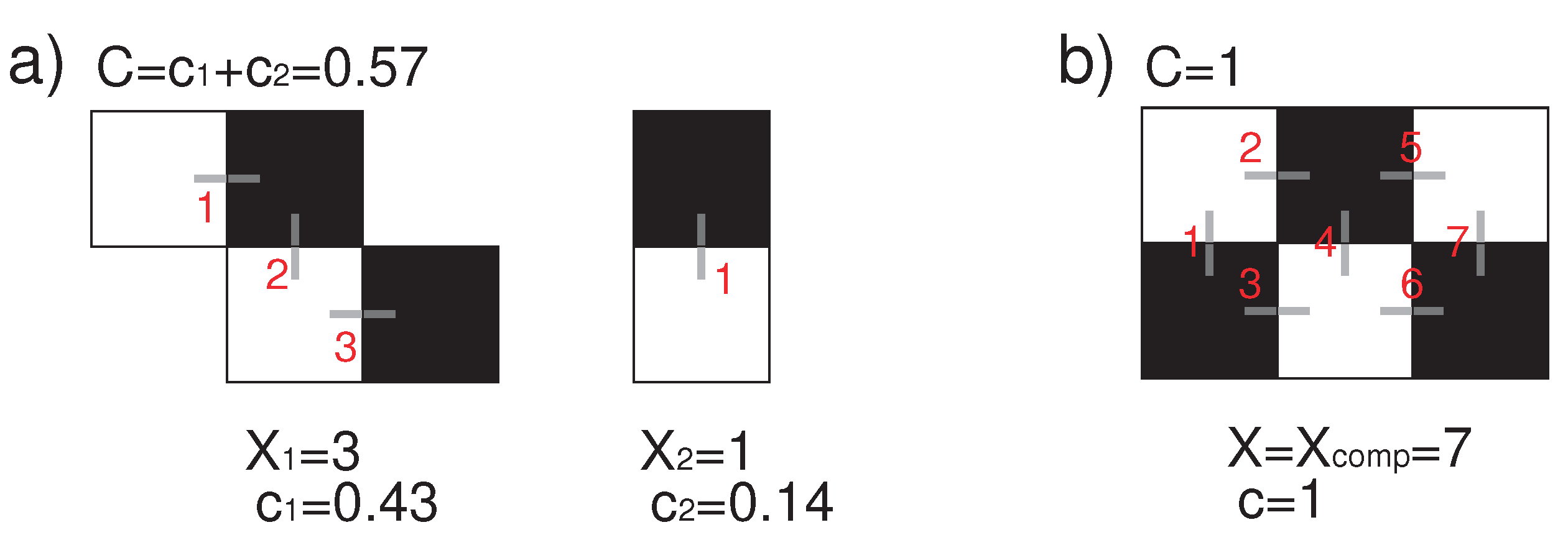
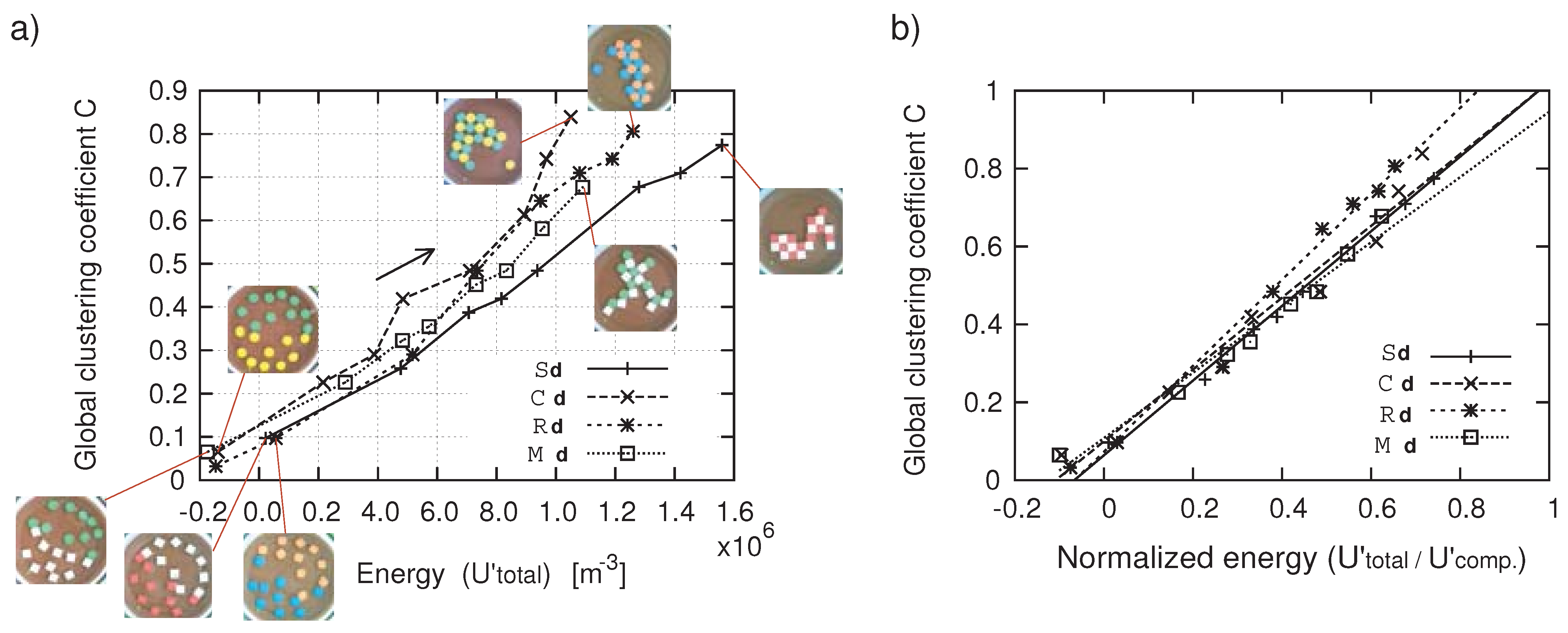
3.2. Clustering coefficients in a self-assembly system

In self-assembly processes, a cluster consists of different components. In addition, components often exhibit different characters and behave differently by linking up together: e.g., proteins open/close their bonding sites flexibly. Systems that contain such multi-states have to be considered together with their initial conditions or physical boundaries, which makes an analytical derivation difficult.

For an answer, one useful insight can be derived from network theory. The idea is to focus only on connections between components (neglecting the identity of each component) and acquiring information about the compounds. To measure the geometrical connections of the tiles, we apply the clustering coefficient concept from network theory [27]. Let $c_i$ be the clustering coefficient of a cluster i. We refer to it as a local clustering coefficient and define it as:

$$\begin{array}{c}\hfill c_i=\frac{\text{number}\text{of}\text{connections}\text{within}\text{the}i\text{-th}\text{cluster}}{\text{number}\text{of}\text{connections}\text{within}\text{the}\text{complete}\text{configuration}}\equiv \frac{x_i}{X_{comp}}\end{array}$$

(7)

X denotes the total number of connections in the system ($X\equiv {\sum }_i{x}_i$). We defined the global clustering coefficient C as the sum of the local clustering coefficients ($C\equiv {\sum }_i{c}_i$).

Figure 2 shows the examples of clustering coefficients with 6 tiles ($X_{comp}=7$). The two local clustering coefficients are $c_1=\frac{3}{7}=0.43$ (left) and $c_2=\frac{1}{7}=0.14$ (right) in (a), while $C=c=\frac{7}{7}=1$ in (b). Note that by defining $X_{comp}$ we focus only on the “targeted” connections between the tiles, that can be recognized in the complete configuration. The concept can be extended and applied to assembly processes in general. In particular, in our experiments with 20 tiles, we assumed that the complete configuration was a lattice structure that was an alignment of $4\times 5$ layers of tiles and had $X_{comp}=31$.

Figure 2. Example of clustering coefficients where $X_{comp}=7$. a) configuration with two clusters where $x_1=3$ (left) and $x_2=1$ (right). b) configuration with $x=X_{comp}=7$. The two local clustering coefficients are $c_1=\frac{3}{7}=0.43$ (left) and $c_2=\frac{1}{7}=0.14$ (right) in (a), while $C=c=\frac{7}{7}=1$ in (b).

Figure 2. Example of clustering coefficients where $X_{comp}=7$. a) configuration with two clusters where $x_1=3$ (left) and $x_2=1$ (right). b) configuration with $x=X_{comp}=7$. The two local clustering coefficients are $c_1=\frac{3}{7}=0.43$ (left) and $c_2=\frac{1}{7}=0.14$ (right) in (a), while $C=c=\frac{7}{7}=1$ in (b).

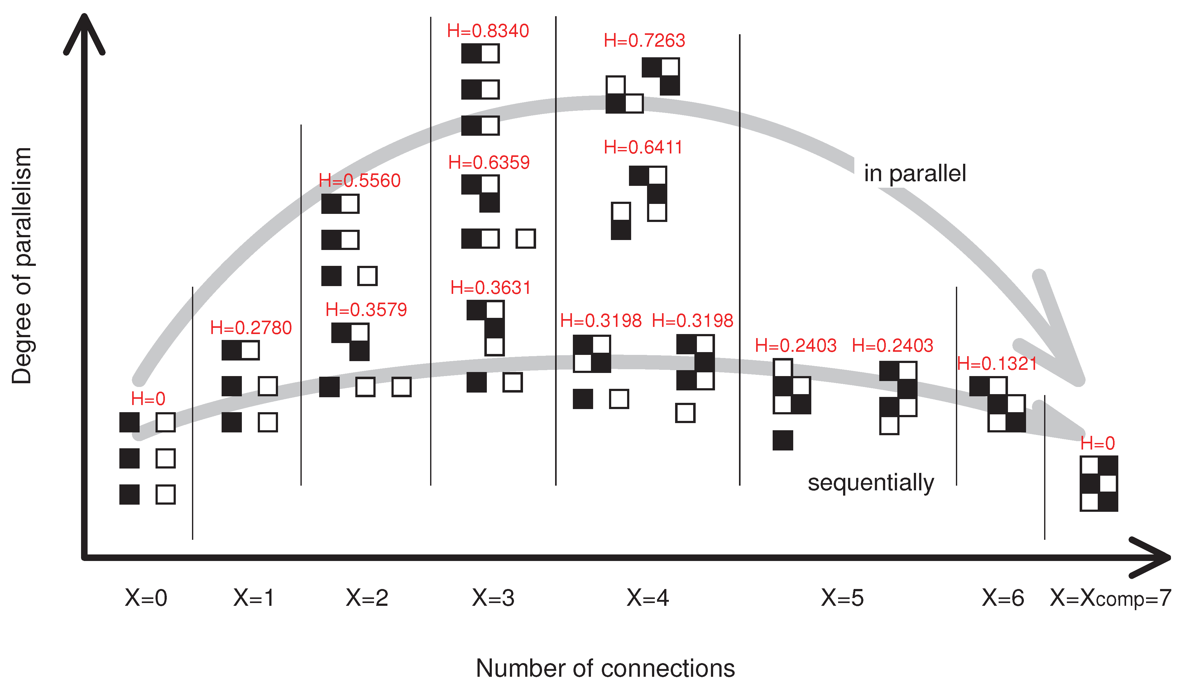
3.3. Entropy and Degree of parallelism (DOP)

Entropy is the common term to express the level of disorder, which is applied in information theory and thermal physics. Adleman [28] described the information-theoretic entropy of a discrete random variable that draws its values from a countable universe. Similar to the entropy concept, we defined the degree of parallelism (DOP) H as a function of the local clustering coefficients ($c_i$), and taking a value between 0 to 1, namely:

$$H=-\sum _{i=1}^N{c}_{i}ln{c}_i$$

(8)

As an illustration of the DOP, consider the situation with an assembly of six tiles, depicted in Figure 3. In the figure, we classify and depict different configurational clusters, according to the number of total connections X. We show each possibility among similar topological clusters, and align considering the number of formed clusters. The figure tells that as X increases, the DOP H increases, attaining a maximum for $X=3$ or $X=4$, and then decreasing to 0 for $X=Xcomp=7$. Also, in each column (that is, within a group having the same number of connections), the more equally clustered, the higher the DOP. In other words, high values are derived from states in which the connections are equally distributed.

Suppose that there exist a number N of clusters. From Shannon’s lemma, it follows that the value H becomes a maximum when N clusters are equally formed, namely;

$$\begin{array}{ccc}\hfill H\left(X\right)& =& -\sum _{i=1}^N{c}_{i}ln{c}_i\hfill \end{array}$$

$$\begin{array}{ccc}& \le & -\sum _{i=1}^N\{\frac{X}{X_{comp}}·\frac{1}{N}\}ln\{\frac{X}{X_{comp}}·\frac{1}{N}\}=-\frac{X}{X_{comp}}ln\{\frac{X}{X_{comp}}·\frac{1}{N}\}\hfill \end{array}$$

(9)

The upper limit in Equation (9), i.e., the maximal value for H, is obtained when $c_i=\{\frac{X}{X_{comp}}·\frac{1}{N}\}$ for $\forall i$, that is, when there are equal numbers of clusters of the same size. This characteristic can be extended to general assembly processes, irrespective of the number of tiles or clusters.

Figure 3. Example of the proposed degree of parallelism H where $X_{comp}=7$. It shows the tendency that the more assembly proceeds in parallel, the larger the value becomes.

Figure 3. Example of the proposed degree of parallelism H where $X_{comp}=7$. It shows the tendency that the more assembly proceeds in parallel, the larger the value becomes.

4. The Experimental Results

We carried out 15 iterative trials for each of 4 different combinations; square tiles and square tiles (${\mathcal{S}}_{·}$ hereafter, ·is either $\mathbf{s}$: with a single magnet or $\mathbf{d}$: with double magnets), circle tiles and circle tiles (${\mathcal{C}}_{·}$), rounded-square tiles and rounded-square tiles (${\mathcal{R}}_{·}$), and square tiles and circle tiles (${\mathcal{M}}_{·}$).

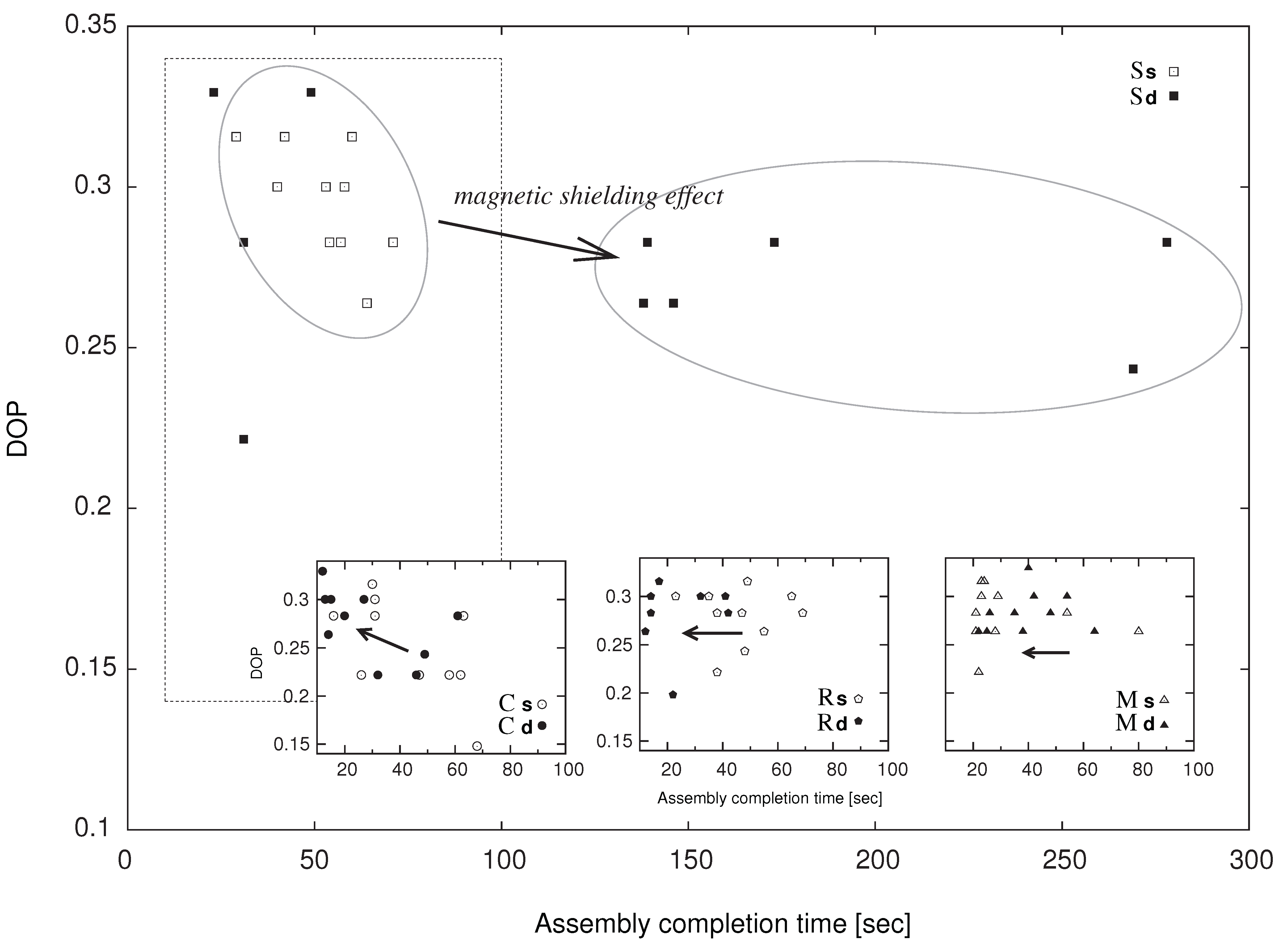
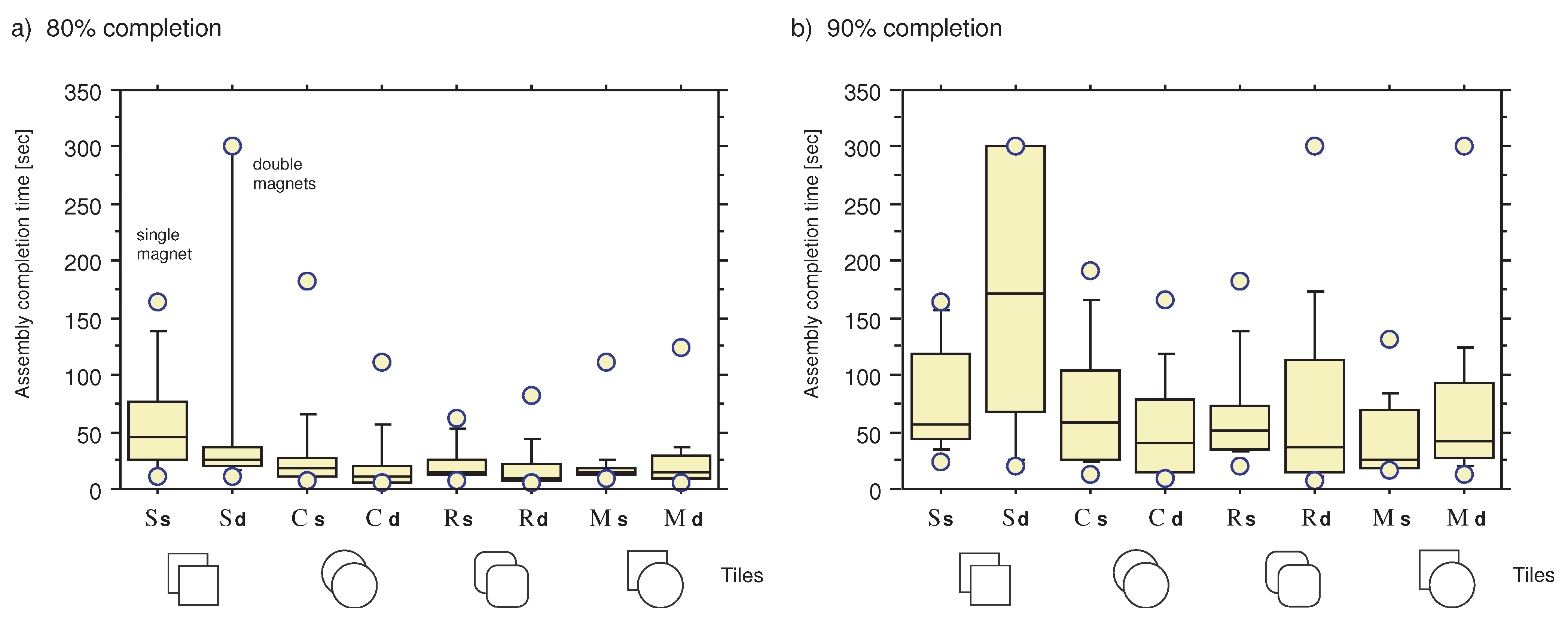
4.1. Assembly completion time

The assembly completion time (completion of over 80% in (a) and 90% in (b)) of all trials are displayed in Figure 4 as a box plot. All the measured data are listed in the Appendix. The boxes on the left side of each column show assembly completion times for single magnet tiles, and on the right side show the times for double magnet tiles. We show the lower quartile (Q1), median (Q2), upper quartile (Q3), and the average of each combination in Table 1. The trials for which we did not observe convergence in a certain amount of time (>300s), are included as 300 s (2 trials in ${\mathcal{S}}_{\text{s}}80\%$ completion, 5 trials in ${\mathcal{S}}_{\text{d}}90\%$ completion, 1 trial in each of ${\mathcal{R}}_{\text{d}}90\%$ and ${\mathcal{M}}_{\text{d}}90\%$ completion).

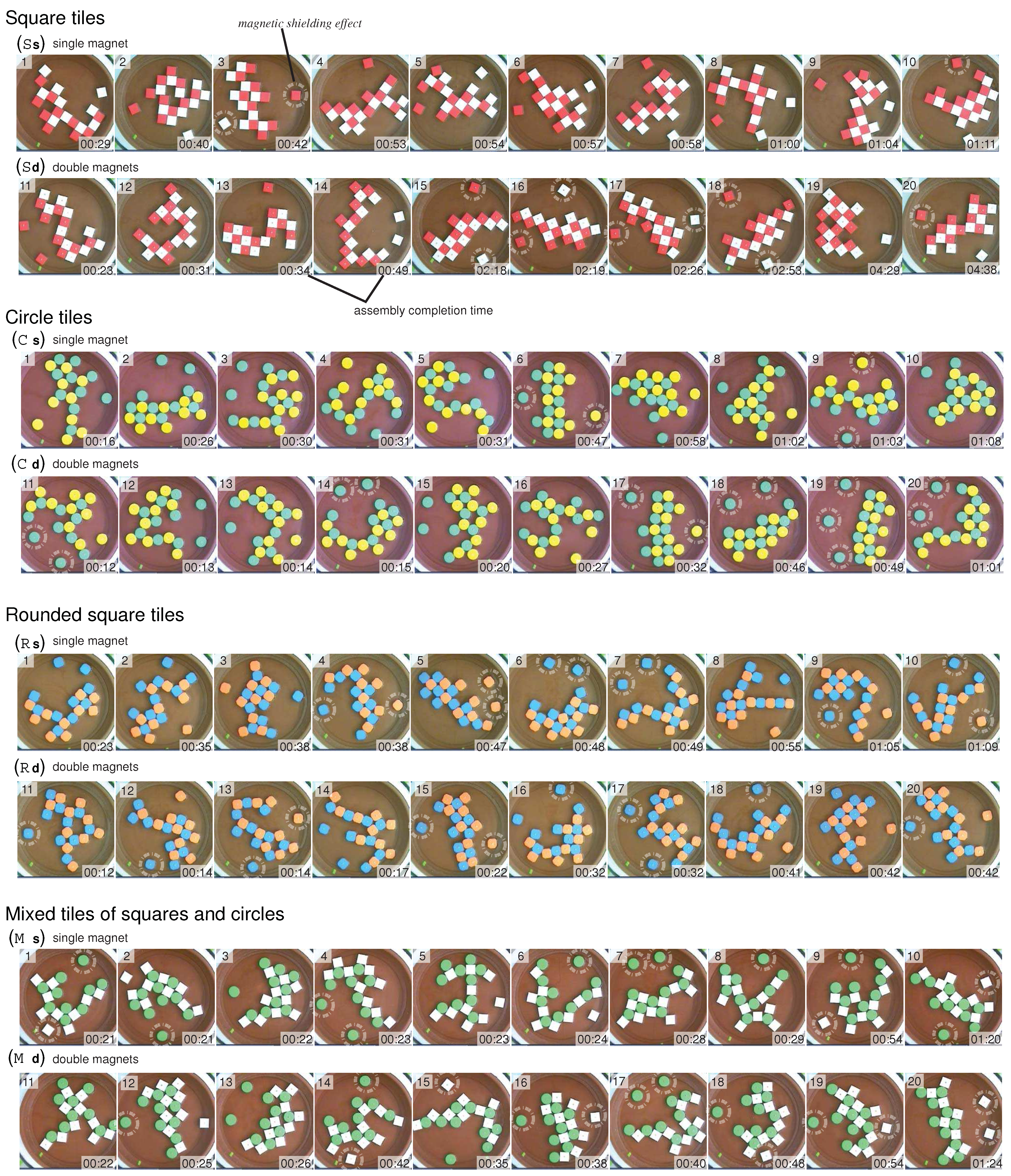
Comparison between different shapes

Regarding the difference in assembly speed from the perspective of the shapes, it is seen that on average, square tiles took the longest time to aggregate compared with the other shaped tiles. However, it should be noted that the shortest completion time of ${\mathcal{S}}_{\text{s}}$ and ${\mathcal{S}}_{\text{d}}$ were as fast as for the other conditions. This is because the minimum distance between the magnets of two connecting tiles was the shortest among all the combinations. Considering the changes in the magnetic attractive force, which is inversely proportional to the distance with a power of 4 (Equation 5), small differences were dominant and induced strong attractive forces. As a factor which hindered the aggregation speed in ${\mathcal{S}}_{\text{d}}$, we observed that frequently the connected tiles were aligned linearly and so prevented other tiles from connecting (magnetic shielding effect, see Figure 5 and Section 5). Once an isolated tile was surrounded by other similarly magnetized tiles connecting each other, the single tile was trapped in the local region and difficult to transfer to a suitable position. This made it difficult for the system to converge and was the main source of such diverse variances. As for the other cases, $\mathcal{C},\mathcal{R},\text{ and }\mathcal{M}$ showed better assembly than $\mathcal{S}.\mathcal{R}$ showed a slightly better assembly capability in speed compared to $\mathcal{C}({\mathcal{C}}_{\text{s}}80\%$ vs. ${\mathcal{R}}_{\text{s}}80\%$, ${\mathcal{C}}_{\text{s}}90\%$ vs. ${\mathcal{R}}_{\text{s}}90\%$, and ${\mathcal{C}}_{\text{d}}80\%$ vs. ${\mathcal{R}}_{\text{d}}80\%$). Here we also saw the effect of the shortest distance between two magnets. $\mathcal{M}$ also showed good assembly speed, mainly due to rotational movement which facilitated reconfiguration in the local region.

Figure 4. Comparison of assembly completion times. a) more than $80\%$ completion. b) more than $90\%$ completion. ($\mathcal{S}$: square, $\mathcal{C}$: circle, $\mathcal{R}$: rounded-square, $\mathcal{M}$: mixed). The boxes on the left side of each column show the assembly completion times for single magnet tiles, and on the right side show the times for double magnet tiles.

Figure 4. Comparison of assembly completion times. a) more than $80\%$ completion. b) more than $90\%$ completion. ($\mathcal{S}$: square, $\mathcal{C}$: circle, $\mathcal{R}$: rounded-square, $\mathcal{M}$: mixed). The boxes on the left side of each column show the assembly completion times for single magnet tiles, and on the right side show the times for double magnet tiles.

Comparison between differently magnetized tiles

We observed two prominent tendencies when comparing conditions with/without a second magnet. Firstly, square tiles with second magnets had an increased assembly completion time, while in the other cases, we saw reductions in their assembly completion time. Secondly, the comparison of percentage rises between $80\%$ completion and $90\%$ completion in Table 1 indicates the difficulty of the last stages’ assembly in each combination, where we observed the big rises in ${\mathcal{R}}_{\text{d}}$ and ${\mathcal{R}}_{\text{s}}$. Taking these two outcomes into account, we can conclude that square tiles and rounded-square tiles had stricter optimal magnetized levels in their assemblies. This originated in the differences in the characteristics of the dynamics; namely, due to the shape and the strong force between two magnets, an alignment of square tiles and rounded-square tiles prevent flexible bends and connection sites. Another noticeable characteristics is that while $\mathcal{R}$ didn’t change the speed so much along with an increase in magnetic force, $\mathcal{M}$ decreased the speed. We think that this is because, whereas rounded-square tiles are able to rotate around neighboring tiles and change their relative positions, a mixed combination with square tiles prohibits this movement and acts as a restriction with a stronger magnetic force.

Table 1. The lower quartile Q1, median, upper quartile Q3, and the averages of $80\%$ and $90\%$ completion level over all of the trials (unit: sec).

	${\mathcal{S}}_{\text{s}}$			${\mathcal{S}}_{\text{d}}$
	80%	90%	increase rate	80%	90%	increase rate
Q1	26	43		19	69
median	45	56		26	172
Q3	83	129		38	300
average*	56.5	76.6	136%	>68.5	>184.2	>269%
	${\mathcal{C}}_{\text{s}}$			${\mathcal{C}}_{\text{d}}$
	80%	90%	increase rate	80%	90%	increase rate
Q1	10	26		6	13
median	18	59		10	41
Q3	29	105		22	80
average	31.2	71.0	228%	20.9	54.2	259%
	${\mathcal{R}}_{\text{s}}$			${\mathcal{R}}_{\text{d}}$
	80%	90%	increase rate	80%	90%	increase rate
Q1	12	33		5	14
median	15	51		9	37
Q3	26	76		19	117
average*	21.5	67.8	315%	18.3	>71.0	>394%
	${\mathcal{M}}_{\text{s}}$			${\mathcal{M}}_{\text{d}}$
	80%	90%	increase rate	80%	90%	increase rate
Q1	12	17		7	25
median	15	26		13	42
Q3	18	77		33	96
average*	21.5	42.7	199%	23.8	>71.4	>300%

*The trials for which we did not observe convergence in a certain amount of time (>300s), are included as 300s (2 trials in ${\mathcal{S}}_{\text{s}}$ 80% completion, 5 trials in ${\mathcal{S}}_{\text{d}}$ 90% completion, 1 trial in each of ${\mathcal{R}}_{\text{d}}$ 90% and ${\mathcal{M}}_{\text{d}}$ 90% completion). All the measured data are listed in the Appendix.

Table 1. The lower quartile Q1, median, upper quartile Q3, and the averages of $80\%$ and $90\%$ completion level over all of the trials (unit: sec).

	${\mathcal{S}}_{\text{s}}$			${\mathcal{S}}_{\text{d}}$
	80%	90%	increase rate	80%	90%	increase rate
Q1	26	43		19	69
median	45	56		26	172
Q3	83	129		38	300
average*	56.5	76.6	136%	>68.5	>184.2	>269%
	${\mathcal{C}}_{\text{s}}$			${\mathcal{C}}_{\text{d}}$
	80%	90%	increase rate	80%	90%	increase rate
Q1	10	26		6	13
median	18	59		10	41
Q3	29	105		22	80
average	31.2	71.0	228%	20.9	54.2	259%
	${\mathcal{R}}_{\text{s}}$			${\mathcal{R}}_{\text{d}}$
	80%	90%	increase rate	80%	90%	increase rate
Q1	12	33		5	14
median	15	51		9	37
Q3	26	76		19	117
average*	21.5	67.8	315%	18.3	>71.0	>394%
	${\mathcal{M}}_{\text{s}}$			${\mathcal{M}}_{\text{d}}$
	80%	90%	increase rate	80%	90%	increase rate
Q1	12	17		7	25
median	15	26		13	42
Q3	18	77		33	96
average*	21.5	42.7	199%	23.8	>71.4	>300%

*The trials for which we did not observe convergence in a certain amount of time (>300s), are included as 300s (2 trials in ${\mathcal{S}}_{\text{s}}$ 80% completion, 5 trials in ${\mathcal{S}}_{\text{d}}$ 90% completion, 1 trial in each of ${\mathcal{R}}_{\text{d}}$ 90% and ${\mathcal{M}}_{\text{d}}$ 90% completion). All the measured data are listed in the Appendix.

4.2. The formed structures

In this section, we evaluate the formed structures of each assembly that is shown in Figure 5. We selected the fastest 10 aggregations out of 15 trials in each combination in order to keep the distributions of the population the same. From top to bottom, the four different combinations are listed and, in each combination, the upper row depicts the case with one magnet and the lower row depicts the double magnet case. In each row, trials are sorted with respect to the increase in assembly completion time.

Figure 5. The formed structures of each assembly of the four different combinations. In each combination, the upper row depicts the case with one magnet and the lower row depicts the double magnet case. The trials are sorted with respect to the increase in assembly completion time. Tiles trapped by the magnetic shielding effect are marked with dotted circles.

Figure 5. The formed structures of each assembly of the four different combinations. In each combination, the upper row depicts the case with one magnet and the lower row depicts the double magnet case. The trials are sorted with respect to the increase in assembly completion time. Tiles trapped by the magnetic shielding effect are marked with dotted circles.

Figure 6. Comparison of DOP against the assembly completion time. Considering the wide time range that square tiles took to complete, we displayed the other combinations in small windows, whose corresponding area is shown as a dotted square.

Figure 6. Comparison of DOP against the assembly completion time. Considering the wide time range that square tiles took to complete, we displayed the other combinations in small windows, whose corresponding area is shown as a dotted square.

In Figure 6, we plotted the DOP of all final configurations versus the time they took to complete. Considering the wide time range that square tiles took to reach a complete assembly, we displayed the other combinations in small windows, whose corresponding area is shown as a dotted square. An increase of DOP was observed for $\mathcal{C}$ and a decrease was observed for $\mathcal{S}$. This suggests that the combination of circular shape with a strong interaction force works not only to accelerate the aggregation speed but also works to achieve a dense structure. Changes were rarely observed with $\mathcal{R}$ and $\mathcal{M}$. The addition of a magnet has several meanings depending on the perspective that is described. In this work, adding a magnet corresponds not only to enhancing the attractive forces among the tiles, which was considered to relatively decay the effect of morphology of the shapes, but also to enhance the effect of shape especially once they connect. That is, it positively influences both the long range interaction due to magnetic forces and the short range interaction through the local shapes.

In some trials, we observed that tiles created gaps within the cluster, such as we can see in Figure 5 ${\mathcal{C}}_{\text{d}}$15, ${\mathcal{R}}_{\text{d}}$11, and ${\mathcal{M}}_{\text{s}}$9. Unlikely to converge into a pure lattice cluster, they frequently created a hall (${\mathcal{S}}_{\text{s}}$2, ${\mathcal{S}}_{\text{d}}$19), or a small gap (${\mathcal{R}}_{\text{s}}$8, ${\mathcal{M}}_{\text{s}}$10). We quantified this tendency by comparing clusters’ surface areas with their perimeters. Note here that the surface area means the entire area inside the cluster, including the gaps. We visually processed the image with Matlab, neglecting stand alone tiles and measured the surface area and the perimeter simply by counting the number of corresponding pixels (Figure 7).

Figure 7. Image processing for the measurement of surface areas and perimeters of clusters. Note here the surface area means the entire area inside the cluster including the gaps.

Figure 7. Image processing for the measurement of surface areas and perimeters of clusters. Note here the surface area means the entire area inside the cluster including the gaps.

In Figure 8, we display perimeters of $\mathcal{S}$ and $\mathcal{C}$ in (a), and $\mathcal{R}$ and $\mathcal{M}$ in (b) compared with the surface areas. Both variables are normalized by the mean values over all combinations and represented as percentages. In general, the further right along the X-axis, the more branched configurations were observed, and the further left, the more rounded were the configurations. The further up the Y-axis, the more gaps are observed.

Figure 8. Comparison of surface areas against perimeters. Both variables are normalized and represented as percentages from mean values. A large negative correlation was observed in $\mathcal{C}$ (−0.573), and a moderate negative correlation was observed in $\mathcal{R}$ (−0:322). Linearly fitted curves of $\mathcal{C}$ and $\mathcal{R}$ are shown in the figures.

Figure 8. Comparison of surface areas against perimeters. Both variables are normalized and represented as percentages from mean values. A large negative correlation was observed in $\mathcal{C}$ (−0.573), and a moderate negative correlation was observed in $\mathcal{R}$ (−0:322). Linearly fitted curves of $\mathcal{C}$ and $\mathcal{R}$ are shown in the figures.

We surmised that the normalized populations followed Gaussian distributions and calculated the correlations of each combination. A large negative correlation was observed for $\mathcal{C}$ (−0.573), and a Entropy 2009, 11 655 moderate negative correlation was observed in $\mathcal{R}$ (−0:322). Linearly fitted curves of $\mathcal{C}$ and $\mathcal{R}$ are shown in the figures as dotted lines. Almost no correlation could be seen in $\mathcal{S}=-0.021$ and $\mathcal{M}-0.036$.

These two fitting lines clearly show reductions in the values of $\mathcal{C}$ and $\mathcal{R}$. This suggests that gaps remained for $\mathcal{C}$ and $\mathcal{R}$ as they formed relatively rounded clusters, whereas in the case of $\mathcal{S}$ and $\mathcal{M}$, gaps were rarely created between tiles, as we see in Figure 8. This is largely due to the characteristics of square tiles. The sharp corners induced a big difference in magnetic force, forcing a strong constraint on the next tiles. For the case of $\mathcal{R}$, they sometimes formed with a 45 degrees rotated formation, resulting in the outcome above.

4.3. Time evolution

In Figure 9, we selected one of the representative aggregations in which more than $95\%$ of tiles were aggregated from each combination and displayed (the respective final configurations can be seen in Figure 5 ${\mathcal{S}}_{\text{d}}$13, ${\mathcal{C}}_{\text{d}}$16, ${\mathcal{R}}_{\text{d}}$15, and ${\mathcal{M}}_{\text{d}}$11). For each case of the raw data, we present the time sequence of trials listed from the left top to the right bottom (with an illustration of the most discriminative movement of the set on the left side). On the right side, we show the transitions of the magnetic potential energy and the clustering coefficients. We discuss each case individually:

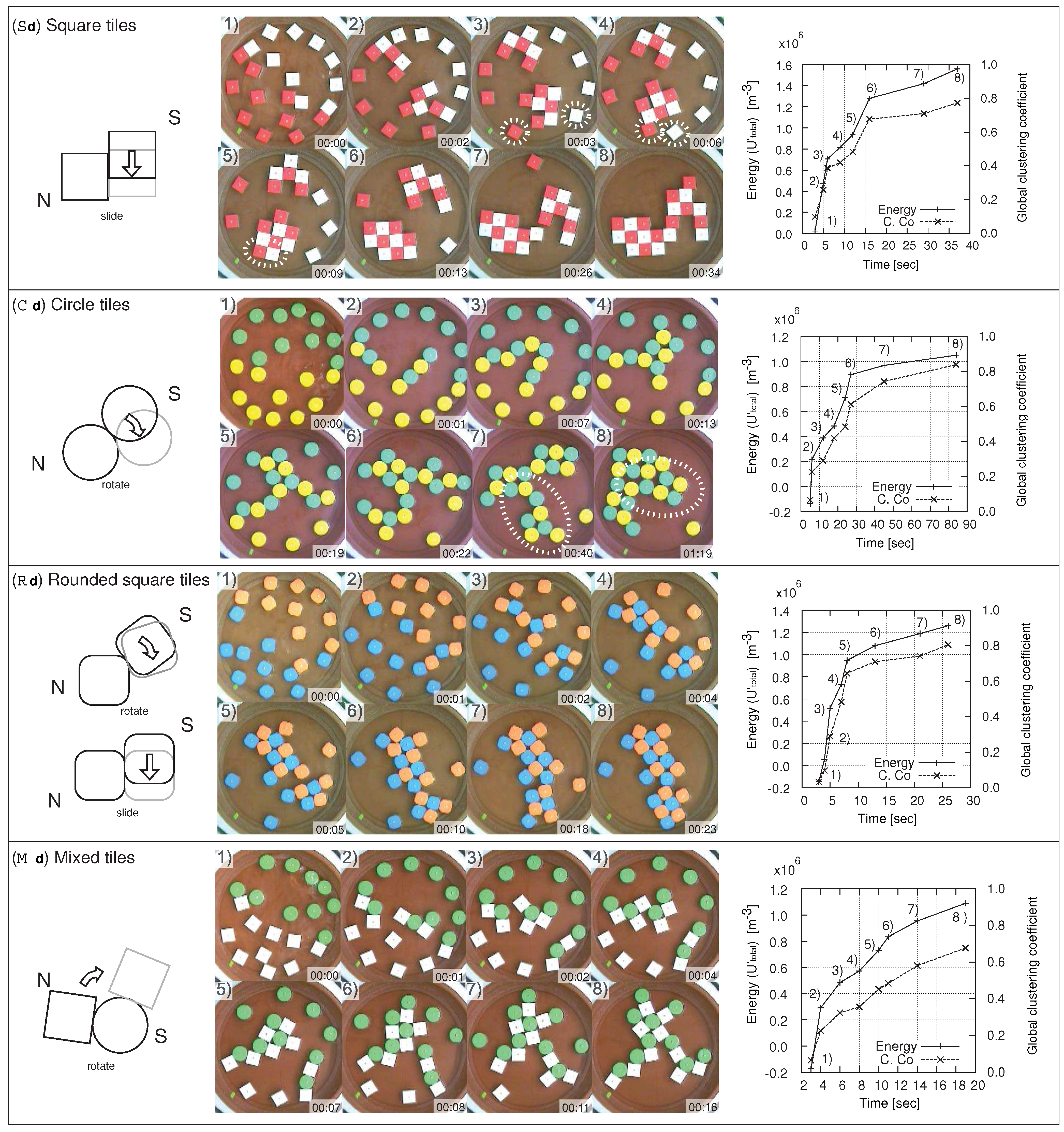
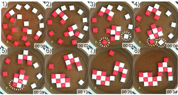
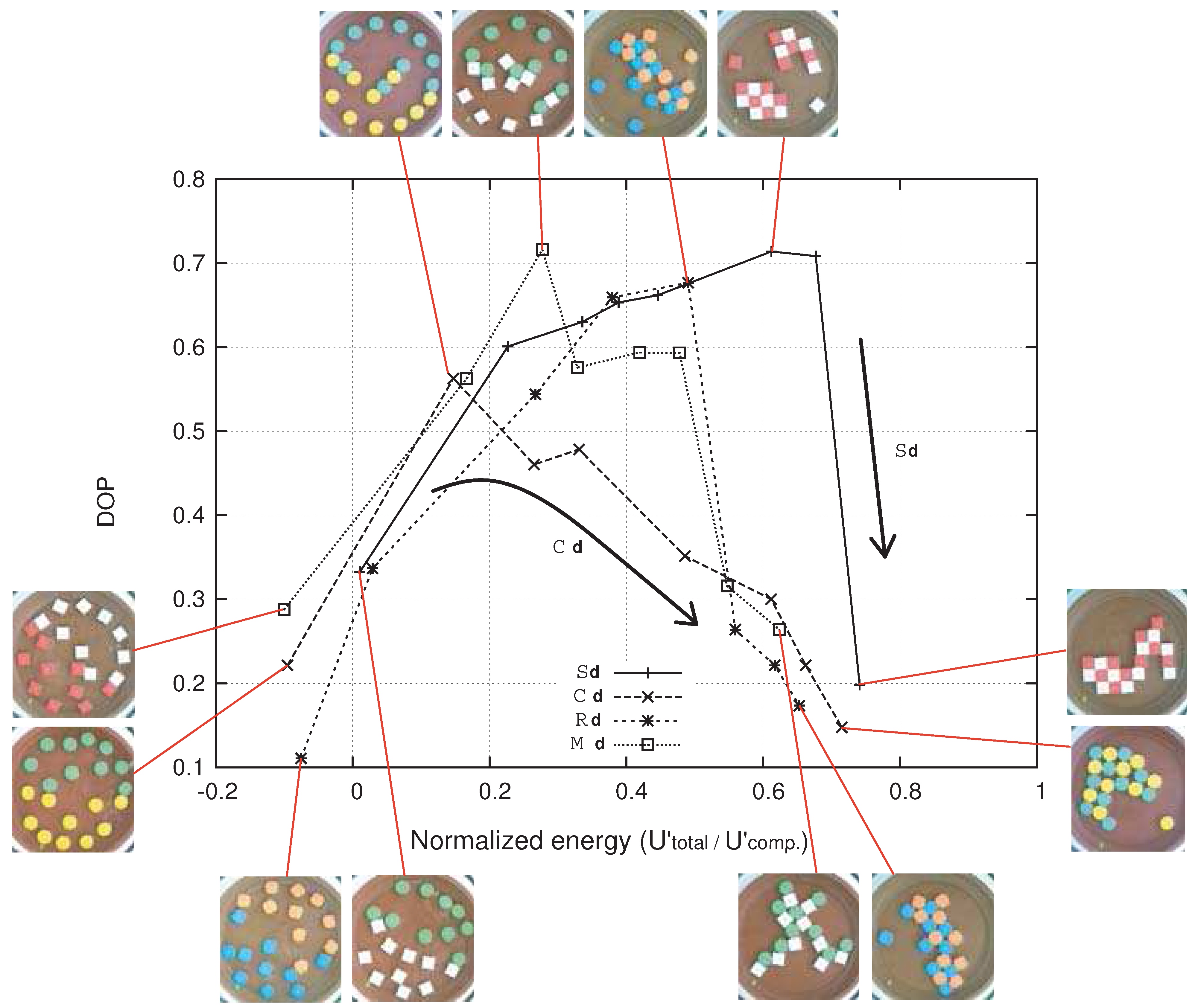
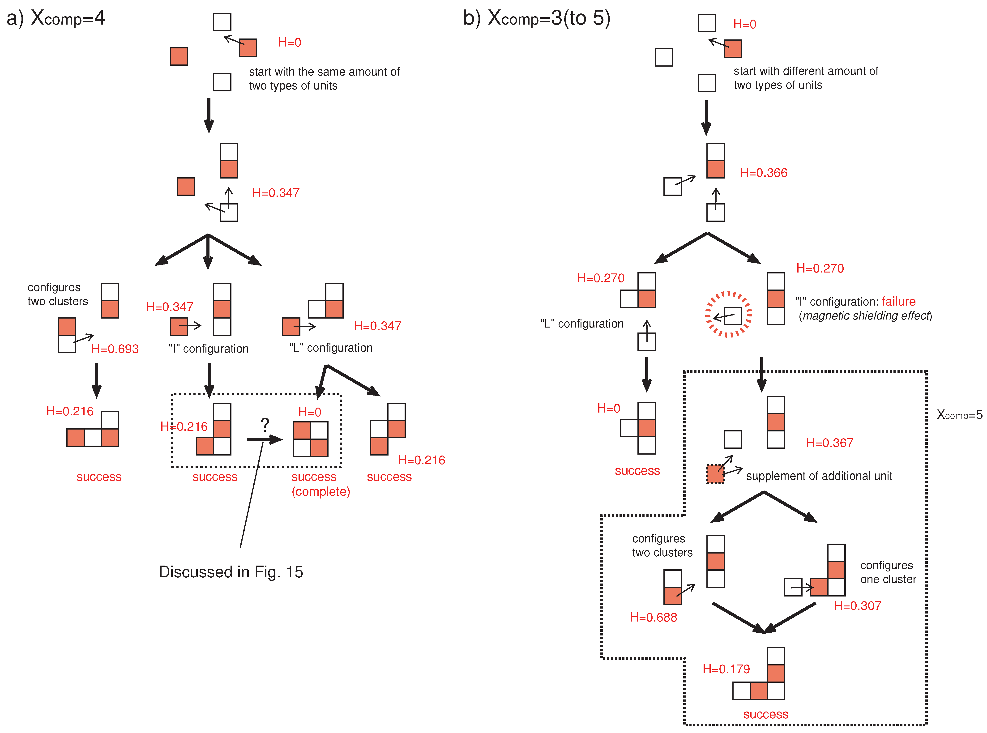
• ${\mathcal{S}}_{\text{d}}$: After the spacer was removed, the tiles moved randomly by changing their relative positions (1–3). The increase in potential energy and the clustering coefficients can be seen in the right figure. Once two tiles were attached (often adjusting their relative positions by sliding), the relatively strong connection force kept the connection tight (2, 7). Note that this results in a large value of the potential energy. This caused the tiles to stay in the same configuration, that is to say, reconfiguration was made more difficult (e.g., 8). As a result, the system produced an irregular shape (8). In this transition, the tiles first formed two small clusters (3–6) and subsequently they bonded together (7). It is worth noting that this large scale docking did not cause a big stored energy jump as expected (reflected in the right figure). This suggests that a major dominance of the energy is induced by locally connecting two tiles but among tiles that are apart. In addition to that, we observed that a white tile highlighted with a dotted circle was assisted to attach to the cluster by a red tile in the transformation from (3) to (5) (magnetic shielding effect, see Section 5).
• ${\mathcal{C}}_{\text{d}}$: In the beginning, several small groups were formed (1–2). The speed of aggregation was fast, whereas connections between two tiles were relatively weak and the tiles changed their relative positions smoothly (3–4 and 6–8). In particular, the transformation highlighted with a dotted circle that can be seen from (7) to (8) is supposed to be rarely observed in the square tile combinations (see Section 5). The increase in potential energy is lower than in the case of square tiles, especially since the closest distance between two magnets is greater (recall that we set the surface area of the tiles to be the same). The transition took 22s for 90% aggregation, and took 79s for the further global configuration (7–8).
• ${\mathcal{R}}_{\text{d}}$: The characteristic of these tiles was that they frequently rotated and changed directions according to the landscape of potential energy (2–4). These tiles possessed positive characteristics of both square and circle tiles, namely, a flexible reconfigurability and a stable lattice formation.

  Figure 9. Representative aggregations of 4 combinations in which more than 95 % of tiles aggregated. For each case of raw data, we present the time sequence of trials listed from the left top to the right bottom (with an illustration of the most discriminative movement of the set on the left side). On the right side, we show the transitions of the magnetic potential energy and the clustering coefficients.

  Figure 9. Representative aggregations of 4 combinations in which more than 95 % of tiles aggregated. For each case of raw data, we present the time sequence of trials listed from the left top to the right bottom (with an illustration of the most discriminative movement of the set on the left side). On the right side, we show the transitions of the magnetic potential energy and the clustering coefficients.

  The lattice structure was reached rapidly (23s) and was sufficiently stable to resist agitation (8). The potential energy converged to a value between those for the cases of square tiles and circle tiles (shown on the right).
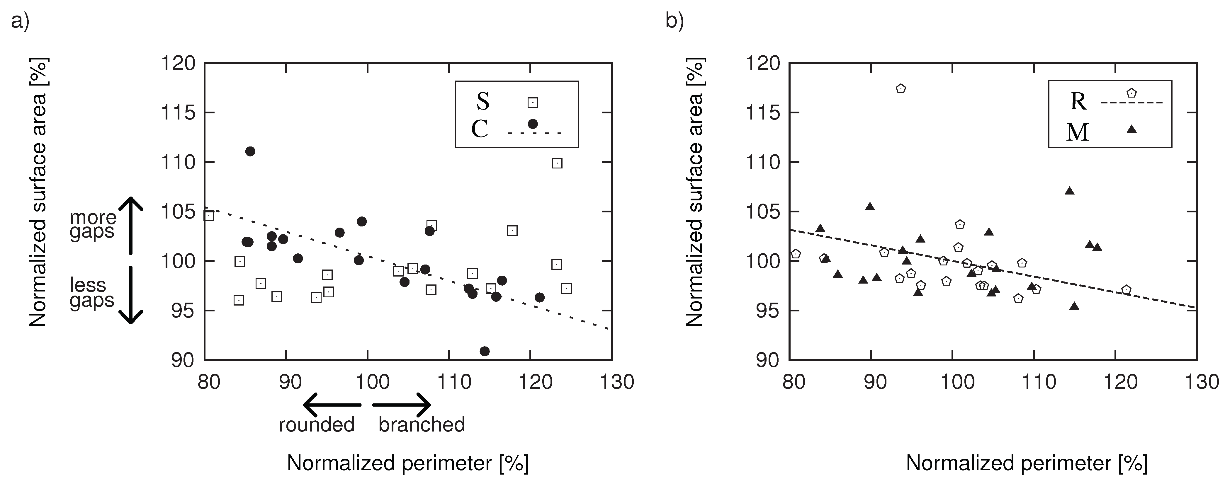
• ${\mathcal{M}}_{\text{d}}$: This was the only heterogeneous combination in terms of shape. Rotation was also observed. The circle tiles acted as a “hinge”, carrying a connected square tile to another position (2–3, 6). Structured lattice regions were stabilized by square tiles fixing the relative positions (8), while due to the flexibility of such combinations, the system often produced branching shapes, which were characterized by lowest clustering coefficients (see Figure 5 ${\mathcal{M}}_{\text{d}}$).

Figure 10 shows the 4 transitions (which are shown in Figure 9) of global clustering coefficients plotted against (a) magnetic potential energies ($U_{total}^{\prime }$), and (b) averaged potential energies ($U_{total}^{\prime }/U_{comp}^{\prime }$).

In Figure 10a, a linear increase in global clustering coefficients was observed (note that ${\mathcal{C}}_{\text{d}}$ took longer time than the others). The linear increase in the number of connections led to an increase in potential energy, showing that the systems were following the terrain of their potential energy to their stable minima. Note that we expect to observe small fluctuations in their energy transitions on the micro scale. Due to the fact that the closest distance between two magnets is the shortest in $\mathcal{S}$ (shape parameter consistency problem, see Section 5), in that situation the largest value of the potential energy existed among the 4 combinations, irrespective of the branched configuration. The gradient of the transition represents the tendency of potential aggregation; here the steeper gradient represents the efficacy of the tiles with respect to aggregation, in contrast to the potential energy. Therefore, for the circle tiles (${\mathcal{C}}_{\text{d}}$), the clusters sustained a tendency to keep reconfiguring, as further agitation occurred. Here, the square tiles (${\mathcal{S}}_{\text{d}}$) seemed to have less probability for reconfiguration (see Section 5 for further discussion). In Figure 10b, linearly fit curves are displayed, along with the plots. Given that the numbers of tiles contained in a cluster were the same, the clustering coefficient tended to be higher, if the cluster had a rounded shape. The inclinations of each plot are 0.958 (${\mathcal{S}}_{\text{d}}$), 0.922 (${\mathcal{C}}_{\text{d}}$), 1.10 (${\mathcal{R}}_{\text{d}}$), and 0.837 (${\mathcal{M}}_{\text{d}}$), respectively, showing that combinations for $\mathcal{R}$ exhibited good aggregation behavior, whereas this was not the case for $\mathcal{M}$.

Figure 10. Comparisons of the 4 transitions of clustering coefficients plotted against (a) potential energy, and (b) normalized potential energy.

Figure 10. Comparisons of the 4 transitions of clustering coefficients plotted against (a) potential energy, and (b) normalized potential energy.

Figure 11 shows the transitions of DOP, where the X-axis represents the magnetic potential energy normalized by the energy of their complete structures ($U_{total}^{\prime }/U_{comp}^{\prime }$).

It can be seen that ${\mathcal{C}}_{\text{d}}$ traces out relatively low values representing a rather sequential aggregation. Note that a large decrease in the value for the last transition of ${\mathcal{S}}_{\text{d}}$ can be observed, where two large clusters combined and eventually resulted in a configuration of one cluster. Considering that both aggregations achieved a quick assembly (27 s in ${\mathcal{C}}_{\text{d}}$ and 34 s in ${\mathcal{S}}_{\text{d}}$), it can be observed that $\mathcal{C}$ proceeds to aggregation at a good pace, irrespective of the aggregation sequence, whereas $\mathcal{S}$ is affected by the sequence (we show this tendency in Figure 14). The attained points for the 4 transitions tell the complete story of their formed structures, suggesting that the reactions were still in a state of local minima. Although it is natural to consider that an increase of the agitation level is needed to overcome this convergence, such a change often leads to the destruction of some appropriate connections as well. This is known to happen, especially when the formed structure has isometry—different configurations with identical connection topologies [29].

Figure 11. Measured clustering coefficients and the DOP plotted against normalized energy.

Figure 11. Measured clustering coefficients and the DOP plotted against normalized energy.

5. Discussion

Toward the aim of general self-assembly principles, we discuss two issues that we encountered during the experiments.

5.1. Shape parameter consistency problem

This problem arose when we simply tried to compare different shapes in the context of self-assembly; i.e., setting the surface area of different shapes to be the same resulted in a variation in diameters. In other words, this variation can be exploited for the desired behaviors in self-assembly. As a consequence, the magnetic force that a square tile can generate on its neighbor is $1.62$ times as large as that of circle tiles. Hence the inducible maximum magnetic force between two tiles could not be made consistent, and thus variation resulted in their stored potential energies.

5.2. Magnetic shielding effect and the influence of shape on self-assembly

The magnetic shielding effect is the effect where the long range magnetic interaction force is effectively canceled by another magnet. This effect was frequently observed with square tiles, which were not flexible with respect to changing their relative positions. This can be illustrated with a simple superposition argument, examining Equation (4) or (5). For example, the total energy in X–Y space can be shown in Figure 12 a, where the three aligned tiles expect another tile (marked as A) to attach (we show $-U_{total}^{\prime }$, for intuitive visualization).

Here we see that the positive energy from the two red tiles acts as a shield, preventing the red tile (A) from connecting to the white tile. The force exerted on a fourth tile, marked by A, is the sum of the three forces—two repulsive and one attractive—from the three connected tiles. If A is at a sufficiently large distance, the repulsive force acts effectively on A, which makes the attachment of A to the rest of the cluster almost impossible (Figure 12b). The tile A needs turbulence which would enable it to overcome the repulsive force and jump into the attractive region of the cluster. What has to be noticed is that this problem can be avoided with a different aggregation sequence. Here, if the first two attachments are made in an “L” instead of a straight configuration, a wider attractive region is kept open for the third red tile (Figure 12c). Furthermore, an additional white tile can expand the attractive region even farther (Figure 12d, “O” configuration). Several fundamental issues can be observed in this phenomenon: the existence of appropriate sets of complementary tiles, the potential role of the aggregation pattern, an adequate agitation level, and the necessity of a physical boundary.

For further investigation, we show two representative convergence paths with 4 square tiles in Figure 13; starting with 2 red and 2 white tiles in (a), and 1 red and 3 white tiles in (b). Here the orders of the paths are expressed with arrows. Each DOP H is also shown for the formed cluster. Surprisingly, in Figure 13a, all paths allow the system to converge. That is, the system has little influence of the magnetic shielding effect, and always completes the aggregation process. However, in Figure 13b, the system has the possibility to be trapped by the problem and doesn’t manage to converge to a single cluster (i.e., a white square tile highlighted with red dotted circle). However, this occasion can be avoided if there is another opponent tile in the system (the dotted red square tile; “supplement of additional unit”). Once this tile is added to the system, no matter to which direction that the system proceeds to assembly, it never encounters the problem. This indicates that having a similar number of sets of opponents on a regular basis helps a system to fall into a local minimum. It also explains why systems proceeded with a fast aggregation in the early stages in the experiments.

Figure 12. Magnetic shielding effect. a) The positive energy from two red tiles (B, C) acts as a shield, preventing the red tile (A) from connecting to the white tile. b) The small attractive region is displayed. The tile A is repelled from the cluster in the grey region. c) If the first two attachments are made with an “L” configuration instead of a straight one, a wider attractive region is kept open for the third red tile. d) An additional white tile can expand the attractive region even farther (“O” configuration).

Figure 12. Magnetic shielding effect. a) The positive energy from two red tiles (B, C) acts as a shield, preventing the red tile (A) from connecting to the white tile. b) The small attractive region is displayed. The tile A is repelled from the cluster in the grey region. c) If the first two attachments are made with an “L” configuration instead of a straight one, a wider attractive region is kept open for the third red tile. d) An additional white tile can expand the attractive region even farther (“O” configuration).

In Figure 14, we plot the DOP transitions of square tiles (shown in Figure 5 ${\mathcal{S}}_{\text{d}}$) vs. the change in the global clustering coefficients. We divide the transitions into two groups, namely, a fast aggregation group (Figure 5 ${\mathcal{S}}_{\text{d}}$ 11 - 14, < 1 min) and a slow aggregation group (Figure 5 ${\mathcal{S}}_{\text{d}}$ 15 - 20, > 2 min), and show the transitions in Figure 14 a and Figure 14 b, respectively. As a reference, we plot mathematically derived DOP curves in which the tiles aggregate in the most sequential way. Note that these curves are the lowest values that the system can take.

The figure indicates that, in the case of rapid transitions, the tiles tended to form two clusters and subsequently aggregated and configured a cluster. This tendency can be seen as large DOP reductions in the second half stages of their transitions, where the global clustering coefficients are between 0.4 and 0.8 (highlighted with a gray colored background). This aggregation pattern can be characterized as parallel growth, where the system proceeds with its assembly utilizing a high degree of parallelism. However, transitions that took a relatively long time (more than 2 minutes) show a tendency to form one large cluster in their early stages, preventing single surrounding tiles from assuming appropriate positions. This comparison clearly shows that the method of aggregation affects the efficiency of self-assembly.

Figure 13. Two examples of square tile assembly. a) Starting with two identical sets of opponent tiles. b) Starting with one red tile and three white tiles.

Figure 13. Two examples of square tile assembly. a) Starting with two identical sets of opponent tiles. b) Starting with one red tile and three white tiles.

In Figure 15, we investigate the possibility of the transformation which we see in Figure 13 (dotted square in (a)). We measured the transitions in magnetic potential energy of square tiles and circle tiles. The energy is normalized by dividing by the absolute initial values ($-U_{total}^{\prime }/\left|U_{total}^{\prime }{|}_{\theta =90}\right|$). Each tile is supposed to move from position A(C) to B(D).

Figure 14. The DOP transitions of square tiles (Figure 5 ${\mathcal{S}}_{\text{d}}$) vs. the change in global clustering coefficients. a) Transitions whose assembly completion times ($90\%$) are less than one minute (Figure 5 ${\mathcal{S}}_{\text{d}}$ 11 - 14). b) Transitions which took more than two minutes (Figure 5 ${\mathcal{S}}_{\text{d}}$ 15 - 20). In the case of rapid transitions, the tiles tended to form two clusters and subsequently aggregated and configured a cluster. This tendency can be observed as large DOP reductions in the second half stages of their transitions, where the global clustering coefficients are between 0.4 and 0.8 (highlighted with a gray colored background).

Figure 14. The DOP transitions of square tiles (Figure 5 ${\mathcal{S}}_{\text{d}}$) vs. the change in global clustering coefficients. a) Transitions whose assembly completion times ($90\%$) are less than one minute (Figure 5 ${\mathcal{S}}_{\text{d}}$ 11 - 14). b) Transitions which took more than two minutes (Figure 5 ${\mathcal{S}}_{\text{d}}$ 15 - 20). In the case of rapid transitions, the tiles tended to form two clusters and subsequently aggregated and configured a cluster. This tendency can be observed as large DOP reductions in the second half stages of their transitions, where the global clustering coefficients are between 0.4 and 0.8 (highlighted with a gray colored background).

Figure 15. Normalized potential energy ($-U_{total}^{\prime }/\left|U_{total}^{\prime }{|}_{\theta =90}\right|$) vs. the rotational angle θ. In the case of square tiles, a potential barrier has to be overcome to arrive at a stable position (B), whereas in the case of circle tiles, the tile can roll down to the position D without any assistance.

Figure 15. Normalized potential energy ($-U_{total}^{\prime }/\left|U_{total}^{\prime }{|}_{\theta =90}\right|$) vs. the rotational angle θ. In the case of square tiles, a potential barrier has to be overcome to arrive at a stable position (B), whereas in the case of circle tiles, the tile can roll down to the position D without any assistance.

The figure indicates that, in the case of square tiles, a potential barrier has to be overcome to arrive at a stable position, whereas in the case of circle tiles, the tile is supposed to roll down to the position D without any assistance (we don’t consider friction). The effect of shape can be clearly recognized here.

6. Conclusions

In this paper, we have shown how the morphology of components affects the self-assembly process. We have proposed a new measure, the degree of parallelism (DOP), which is a function of clustering coefficients, to quantify the aggregation characteristics,. The DOP captures how the system allocates connections into different clusters. The results acquired using this measure showed that the early stages of the aggregation pattern are crucially influential to the rest of the entire assembly process. It was observed that a shape which has a rounded corner, such as a circle or rounded-square eases the problem—the Magnetic shielding effect—and facilitates efficient assembly at an appropriate magnetized level. We clearly show that a change in the morphology of components can induce different aggregation patterns, affecting the completed structure of their final configurations.

References

1. Whitesides, G.M.; Grzybowski, B. Self-assembly at all scales. Science 2002, 295, 2418–2421. [Google Scholar] [CrossRef] [PubMed]
2. Leiman, P.G.; Kanamaru, S.; Mesyanzhinov, V.V.; Arisaka, F.; Rossmann, M.G. Structure and morphogenesis of bacteriophage t4. Cell. Mol. Life Sci. 2003, 60, 2356–2370. [Google Scholar] [CrossRef] [PubMed]
3. Nakagawa, A.; Miyazaki, N.; Taka, J.; Naitow, H.; Ogawa, A.; Fujimoto, Z.; Mizuno, H.; Higashi, T.; Watanabe, Y.; Omura, T.; Cheng, R.H.; Tsukihara, T. The atomic structure of rice dwarf virus reveals the self-assembly mechanism of component proteins. Structure 2003, 11, 1227–1238. [Google Scholar] [CrossRef] [PubMed]
4. Alberts, B.; Hohnson, A.; Lewis, J.; Raff, M.; Roberts, K.; Walter, P. Molecular Biology of the Cell; Garland Science: New York, NY, USA, 2002. [Google Scholar]
5. Penrose, L.S. Self-reproducing. Sci. Amer. 1959, 200-6, 105–114. [Google Scholar] [CrossRef]
6. Hosokawa, K.; Shimoyama, I.; Miura, H. Dynamics of self-assembling systems: Analogy with chemical kinetics. Artif. Life 1994, 1, 413–427. [Google Scholar] [CrossRef]
7. Hosokawa, K.; Shimoyama, I.; Miura, H. 2-d micro-self-assembly using the surface tension of water. Sens. Actuators. A 1996, 57, 117–125. [Google Scholar] [CrossRef]
8. Bowden, N.; Terfort, A.; Carbeck, J.; Whitesides, G.M. Self-assembly of mesoscale objects into ordered two-dimensional arrays. Science 1997, 276, 233–235. [Google Scholar] [CrossRef] [PubMed]
9. Grzybowski, B.A.; Stone, H.A.; Whitesides, G.M. Dynamic self-assembly of magnetized, millimetre-sized objects rotating at a liquid-air interface. Nature 2000, 405, 1033. [Google Scholar] [PubMed]
10. Grzybowski, B.A.; Winkleman, A.; Wiles, J.A.; Brumer, Y.; Whitesides, G.M. Electrostatic self-assembly of macroscopic crystals using contact electrification. Nature 2003, 2, 241–245. [Google Scholar] [CrossRef] [PubMed]
11. Grzybowski, B.A.; Radkowski, M.; Campbell, C.J.; Lee, J.N.; Whitesides, G.M. Self-assembling fluidic machines. Appl. Phys. Lett. 2004, 84, 1798–1800. [Google Scholar] [CrossRef]
12. Saitou, K. Conformational switching in self-assembling mechanical systems. IEEE Trans. Rob. Autom. 1999, 15, 510–520. [Google Scholar] [CrossRef]
13. Winfree, E.; Liu, F.; Wenzler, L.A.; Seeman, N.C. Design and self-assembly of two-dimensional dna crystals. Nature 1998, 394, 539–544. [Google Scholar] [CrossRef] [PubMed]
14. Seeman, N.C. DNA in a material world. Nature 2003, 421, 427–430. [Google Scholar] [CrossRef] [PubMed]
15. Mao, C.; LaBean, T.H.; Reif, J.H.; Seeman, N.C. Logical computation usingalgorithmic self-assembly. Nature 2000, 407, 493–496. [Google Scholar] [PubMed]
16. Shih, W.M.; Quispe, J.D.; Joyce, G.F. A 1.7-kilobase single-stranded dna that folds into a nanoscale octahedron. Nature 2004, 427, 618–621. [Google Scholar] [CrossRef] [PubMed]
17. Rothemund, P. W.K. Folding dna to create nanoscale shapes and patterns. Nature 2006, 440, 297–302. [Google Scholar] [CrossRef] [PubMed]
18. Yokoyama, T.; Yokoyama, S.; Kamikado, T.; Okuno, Y.; Mashiko, S. Selective assembly on a surface of supramolecular aggregates with controlled size and shape. Nature 2001, 413, 619–621. [Google Scholar] [CrossRef] [PubMed]
19. White, P.; Kopanski, K.; Lipson, H. Stochastic self-reconfigurable cellular robotics. In Proc. IEEE Int. Conf. Rob. Autom. (ICRA); New Orleans, LA, USA, 2004; Volume 3, pp. 2888–2893. [Google Scholar]
20. White, P.; Zykov, V.; Bongard, J.; Lipson, H. Three dimensional stochastic reconfiguration of modular robots. In Proc. Int. Conf. Rob. Sci. Sys. (RSS); The MIT Press: Cambridge, MA, USA, 2005; pp. 161–168. [Google Scholar]
21. Shimizu, M.; Ishiguro, A. A modular robot that exploits a spontaneous connectivity control mechanism. In Proc. IEEE Int. Conf. Rob. Autom. (ICRA); Barcelona, Spain, 2005; pp. 2658–2663. [Google Scholar]
22. Bishop, J.; Burden, S.; Klavins, E.; Kreisberg, R.; Malone, W.; Napp, N.; Nguyen, T. Programmable parts: A demonstration of the grammatical approach to self-organization. In Proc. IEEE/RSJ Int. Conf. Intell. Rob. Sys. (IROS); Edmonton, AB, Canada, 2005; pp. 3684–3691. [Google Scholar]
23. Griffith, S.; Goldwater, D.; Jacobson, J. Robotics: Self-replication from random parts. Nature 2005, 437, 636. [Google Scholar] [CrossRef] [PubMed]
24. Nagy, Z.; Oung, R.; Abbott, J.J.; Nelson, B.J. Experimental investigation of magnetic self-assembly for swallowable modular robots. In Proc. IEEE/RSJ Int. Conf. Intell. Rob. Sys. (IROS); Nice, France, 2008. [Google Scholar]
25. Miyashita, S.; Kessler, M.; Lungarella, M. How morphology affects self-assembly in a stochastic modular robot. In Proc. IEEE Int. Conf. Rob. Autom. (ICRA); Pasadena, CA, USA, 2008. [Google Scholar] [Green Version]
26. Miyashita, S.; Casanova, F.; Lungarella, M.; Pfeifer, R. Peltier-based freeze-thaw connector for waterborne self-assembly systems. In Proc. IEEE Int. Conf. Intell. Rob. Sys. (IROS); Nice, France, 2008; pp. 1325–1330. [Google Scholar]
27. Watts, D.J.; Strogatz, S.H. Collective dynamics of ’small-world’ networks. Nature 1998, 393, 440–441. [Google Scholar] [CrossRef] [PubMed]
28. Adleman, L. Linear self-assemblies: Equilibria, entropy and convergence rates. In Proc. Sixth Int. Conf. on Differ. Equ.; Taylor and Francis: London, UK, 2001. [Google Scholar]
29. Fujibayashi, K.; Murata, S.; Sugawara, K.; Yamamura, M. Self-organizing formation algorithm for active elements. Forma 2003, 18, 83–95. [Google Scholar]
Appendix
The assembly completion time [sec] (80% and 90% completion) of all combinations.
S s S d C s C d
trials80%90%80%90%80%90%80%90%
11234191369261656
24545142162827610
35156334619541329
4191291920181092224
52653171722959713
6112438266182656119
746552727102326117
8585826>30023166611
99090>300>30029971180
108315726261821921146
1136672030012131041
121381382113525105711
13164164292731459617
142636113006565573
154343>300>3001644111166
average*56.576.6>68.5>184.231.271.020.954.2
R s R d M s M d
1141838213910172038
2181388141377720
31343102812173696
42665101741236581
582019391884124124
6124651117261425
72432911142610106
827765826481342
9154581720233450
1013130223715811534
1112515371717812
1215339>30010173337
13626243104122119>300
141233111171121321321
15526029291519665
average*21.567.818.3>71.021.542.723.8>71.4
*The trials which took longer than 300 s are included as 300 s (listed with “>”).