Exergy as a Useful Variable for Quickly Assessing the Theoretical Maximum Power of Salinity Gradient Energy Systems

Abstract
:1. Introduction
2. Defining the System
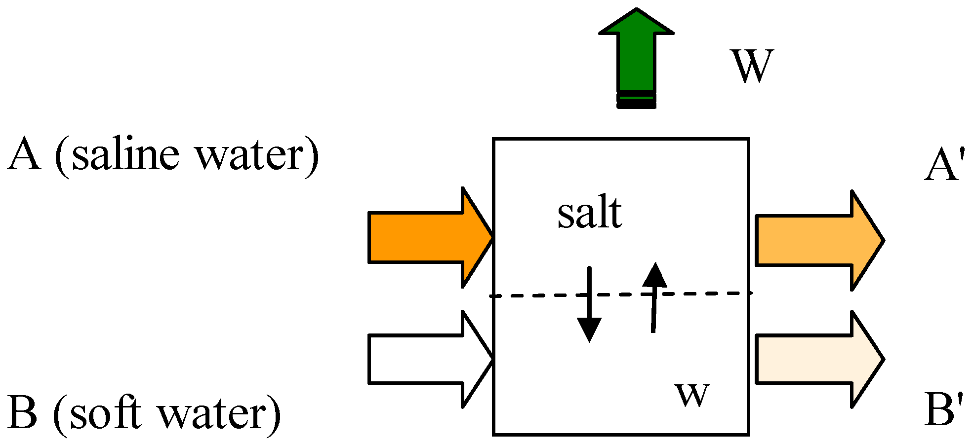
- (i)
- Pressure and temperature for each of streams A, A’, B and B’
- (ii)
- Mass flowrate and composition of each of the inlet streams A and B
- (iii)
- Mass flowrate and direction of each of the internal stream describing respectively transport of water and transport of salt.
2. Assessing Mass Balance
3. Assessing the Exergy Balance
4. Examples
4.1. Presentation of the examples and methodology

| Units | Symbol | General system (mixing) | PRO type system | RED type system | |
|---|---|---|---|---|---|
| Mass flow–seawater (stream A) | kg/s | FA | FA >> FB | 1,000 | 1,000 |
| Salinity–stream A | g/kg | ξA | 35 | 35 | 35 |
| Mass flow–soft water (stream B) | kg/s | FB | 1,000 | 1,000 | 1,000 |
| Salinity–stream B | g/kg | ξB | 0 | 0 | 0 |
| Salt transfer ratio from A to B | τs | 0 | 0 | variable | |
| Water transfer ratio from B to A | τw | → 1 | variable | 0 | |
| Temperature | °C | θ | 10 | 10 | 10 |
| Pressure | atm | p | 1 | 1 | 1 |
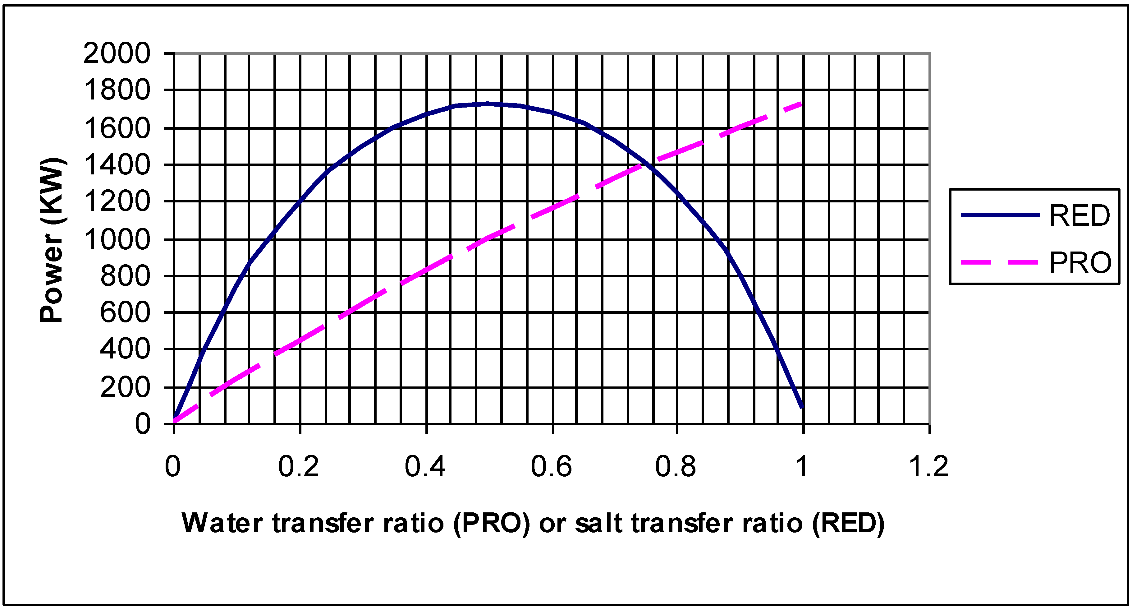
| Calculated maximum power | kW | W | 2,341 | figure | figure |
4.2. First example: system allowing transfer of pure water into a sink of oceanic water

4.3. Second example: a PRO type system
| τw | h (100 kJ/kg) | s (100 kJ/kg–K) | et + ech (kJ/kg) |
|---|---|---|---|
| 0 | –4.6184 | 1.8096 | –5.1673 |
| 0.1 | –1.4631 | 1.7276 | –4.9037 |
| 0.2 | 0.6918 | 1.6533 | –4.6720 |
| 0.3 | 2.1841 | 1.5856 | –4.4653 |
| 0.4 | 3.2258 | 1.5234 | –4.2791 |
| 0.5 | 3.9543 | 1.4662 | –4.1098 |
| 0.6 | 4.4612 | 1.4133 | –3.9549 |
| 0.7 | 4.8088 | 1.3642 | –3.8125 |
| 0.8 | 5.0408 | 1.3185 | –3.6809 |
| 0.9 | 5.1877 | 1.2759 | –3.5589 |
| → 1 | 5.2719 | 1.2361 | –3.4454 |
4.4. Second example: RED type system
| Streams → | A’ | B’ | ||||
|---|---|---|---|---|---|---|
| τs | h (100 kJ/kg) | s (100 kJ/kg–K) | et + ech (kJ/kg) | h (100 kJ/kg) | s (100 kJ/kg–K) | et + ech (kJ/kg) |
| 0 | –4.6184 | 1.8096 | –5.1673 | 0.0000 | 0.0000 | 0.0000 |
| 0.1 | –1.2789 | 1.7220 | –4.8860 | 1.6731 | 0.3684 | –1.0258 |
| 0.2 | 1.3734 | 1.6246 | –4.5840 | 3.2759 | 0.6449 | –1.7923 |
| 0.3 | 3.3406 | 1.5154 | –4.2551 | 4.4765 | 0.8707 | –2.4192 |
| 0.4 | 4.6285 | 1.3915 | –3.8918 | 5.1664 | 1.0604 | –2.9493 |
| 0.5 | 5.2485 | 1.2497 | –3.4842 | 5.2896 | 1.2227 | –3.4075 |
| 0.6 | 5.2204 | 1.0855 | –3.0198 | 4.8136 | 1.3634 | –3.8102 |
| 0.7 | 4.5776 | 0.8929 | –2.4810 | 3.7186 | 1.4865 | –4.1696 |
| 0.8 | 3.3783 | 0.6628 | –1.8418 | 1.9931 | 1.5954 | –4.4949 |
| 0.9 | 1.7360 | 0.3796 | –1.0569 | –0.3693 | 1.6925 | –4.7934 |
| 1 | 0.0000 | 0.0000 | 0.0000 | –3.3714 | 1.7799 | –5.0709 |
5. Conclusions
Acknowledgements
References and Notes
- Loeb, S. Osmotic power plants. Science 1975, 189, 654–655. [Google Scholar] [CrossRef] [PubMed]
- Loeb, S. Production of energy from concentrated brines by pressure retarded osmosis. J. Membrane Sci. 1976, 1, 49–63. [Google Scholar] [CrossRef]
- Loeb, S. Method and apparatus for generating power utilizing pressure-retarded osmosis. US Patent 4,193,267, 1980. [Google Scholar]
- Loeb, S. Energy production at dead sea by pressure-retarded osmosis: Challenge or chimera? Desalination 1998, 120, 247–262. [Google Scholar] [CrossRef]
- Loeb, S.; Honda, T.; Reali, M. Comparative mechanical efficiency of several plant configurations using a pressure-retarded osmosis converter. J. Membrane Sci. 1990, 51, 223–335. [Google Scholar] [CrossRef]
- Loeb, S. Large scale production by pressure-retarded osmosis, using river water and sea water passing through spiral modules. Desalination 2002, 143, 115–122. [Google Scholar] [CrossRef]
- Stover, R.L.; Pique, G.G. Osmotic power from the ocean. Power 2006, 150, 76–80. [Google Scholar]
- Panyor, L. Renewable energy from dilution of salt water with fresh water: Pressure retarded osmosis. Desalination 2006, 199, 408–410. [Google Scholar] [CrossRef]
- Cameron, I.B.; Clemente, R.B. SWRO with ERI’s PX pressure exchanger device–a global survey. Desalination 2008, 221, 136–142. [Google Scholar] [CrossRef]
- Skilgahen, S.E.; Dugstad, J.E.; Aaberg, R.J. Osmotic power–power production based on osmotic pressure difference between waters with varying salt gradients. Desalination 2008, 220, 476–482. [Google Scholar] [CrossRef]
- Post, J.W.; Veerman, J.; Hamelers, H.V.M.; Euverink, G.J.W.; Metz, S.J.; Nymeijer, K.; Buisman, C.J.N. Salinity-gradient power: Evaluation of pressure-retarded osmosis and reverse electrodialysis. J. Membrane Sci. 2007, 288, 218–230. [Google Scholar] [CrossRef]
- Weinstein, J.N.; Leitz, F.B. Electric power from differences in salinity: The dialytic battery. Science 1976, 191, 557–559. [Google Scholar] [CrossRef] [PubMed]
- Lacey, R.E. Energy by reverse electrodialysis. Ocean Energy 1980, 7, 1–47. [Google Scholar] [CrossRef]
- Turek, M.; Bandura, B. Renewable energy by reverse electrodialysis. Desalination 2007, 205, 67–74. [Google Scholar] [CrossRef]
- Jones, A.T.; Finley, W. Recent developments in salinity gradient power. Oceans 2003, 4, 2284–2287. [Google Scholar]
- Olson, M.; Wick, G.L.; Isaacs, J.D. Salinity gradient power: Utilizing vapour pressure differences. Science 1979, 206, 452–454. [Google Scholar] [CrossRef] [PubMed]
- Labrecque, R.; Boulama, K.G. Get the most out of waste heat. Chem. Eng. 2006, 11, 40–43. [Google Scholar]
- Millero, F.J.; Leung, W. The thermodynamics of seawater at one atmosphere. Amer. J. Sci. 1976, 276, 1035–1077. [Google Scholar] [CrossRef]
© 2009 by the authors; licensee Molecular Diversity Preservation International, Basel, Switzerland. This article is an open-access article distributed under the terms and conditions of the Creative Commons Attribution license (http://creativecommons.org/licenses/by/3.0/).
Share and Cite
Labrecque, R. Exergy as a Useful Variable for Quickly Assessing the Theoretical Maximum Power of Salinity Gradient Energy Systems. Entropy 2009, 11, 798-806. https://doi.org/10.3390/e11040798
Labrecque R. Exergy as a Useful Variable for Quickly Assessing the Theoretical Maximum Power of Salinity Gradient Energy Systems. Entropy. 2009; 11(4):798-806. https://doi.org/10.3390/e11040798
Chicago/Turabian StyleLabrecque, Raynald. 2009. "Exergy as a Useful Variable for Quickly Assessing the Theoretical Maximum Power of Salinity Gradient Energy Systems" Entropy 11, no. 4: 798-806. https://doi.org/10.3390/e11040798