Lorenz Curves, Size Classification, and Dimensions of Bubble Size Distributions

Physikalische Chemie, Fritz-Haber-Institut der Max-Planck-Gesellschaft, Faradayweg 12, D-14195 Berlin, Germany
Entropy 2010, 12(1), 1-13; https://doi.org/10.3390/e12010001
Submission received: 13 October 2009
/
Accepted: 11 December 2009
/
Published: 25 December 2009
Abstract
:Lorenz curves of bubble size distributions and their Gini coefficients characterize demixing processes. Through a systematic size classification, bubble size histograms are generated and investigated concerning their statistical entropy. It turns out that the temporal development of the entropy is preserved although characteristics of the histograms like number of size classes and modality are remarkably reduced. Examinations by Rényi dimensions show that the bubble size distributions are multifractal and provide information about the underlying structures like self-similarity.
1. Introduction
It has been shown that the application of majorization [1,2,3,4,5,6] to time series of bubble size distributions leads to very intriguing insights into decaying foam [7,8,9,10,11,12,13,14,15]. The decay of liquid foams is comprised of two processes: drainage at the beginning and subsequent ageing. Generating foam by ultrasound treatment enables a separation of the two decay processes. Not only measuring the shrinking foam volume [7,8,9] but also the evaluation of bubble size histograms by classical majorization and its order-preserving functions has revealed a temporal separation of drainage and ageing [11,12]. As a first approach ten size classes were chosen for forming bubble size histograms. Then drainage is characterized by classical majorization in time, histograms from the ageing phase are predominantly incomparable. As an order-preserving function of classical majorization the Shannon entropy [16] was used for mapping the histograms onto real values. Since drainage corresponds to a classical majorization in time the Shannon entropy values increase, but the incomparableness during the ageing phase shows a decrease which is accompanied by an irregular behaviour.
In [14] the same foam experiment was used but the area imaged by the camera and the size classes of the bubble size histograms were smaller by a factor of 4 respectively 2. With these conditions a process separation could not be found, instead a monotonously increasing Shannon entropy behaviour was found. Hence, the question arises whether the process separation depends on the image size or on the chosen data binning. In general, if data binning is to be chosen for bubble sizes do there exist criteria for an optimal bin width. Does there exist a certain data binning which leads to other foam characteristics?
In this paper systematic data binning is applied to bubble size distributions which are obtained under the conditions described in [14]. In order to get insights into the temporal development of the raw data, concepts are used which go back to Lorenz [17] and Dalton [18] and represent a predecessor of majorization. Originally introduced to measure inequality of income or wealth, Lorenz curves are used to describe the underlying statistical process of bubble size distributions. Then bubble size histograms are generated in which the bin width depends on the smallest element (bubble). The development of both Lorenz curves and histograms of different bin classifications are evaluated by corresponding entropy measures: the Gini coefficient [19] for Lorenz curves and the Shannon entropy [16] for histograms.
This work is organized as follows: first the mathematical background is introduced (Section 2.). In Section 3. Lorenz curves and Gini coefficients of bubble size distributions are generated, followed by systematic size classification for bubble size histograms. The latter leads to both a possibility to find a criterion for an optimal size classification and a further foam characteristic using the concept of Rényi dimensions [21], see Section 4.. An optimal size classification is suggested and a simple model depicting the structure of the raw data is discussed in Section 5., followed by a conclusion.
2. Mathematical Background
In the following, the notations of Lorenz curves and histograms with their entropy measures are introduced. The original example of income distributions of a population is used.
2.1. Lorenz Curve and Gini Coefficient
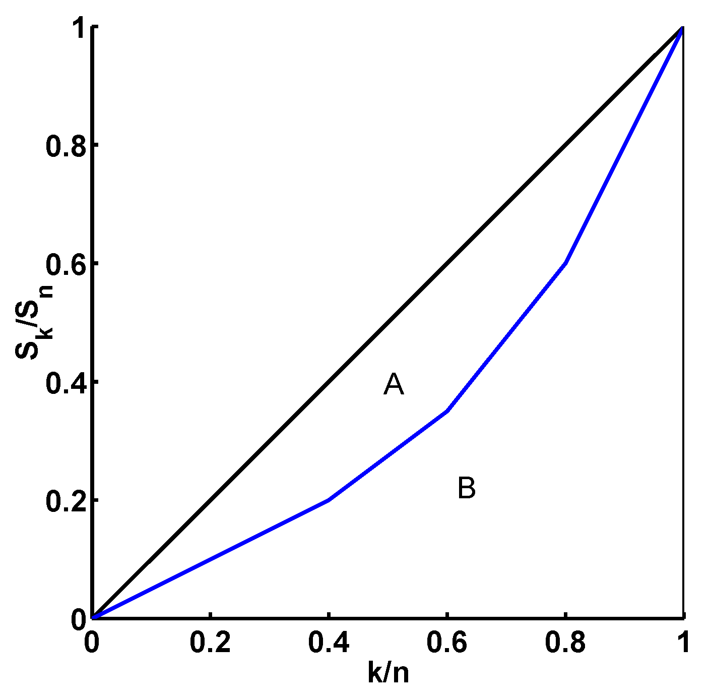
The Lorenz curve [17] is a method to describe inequality in wealth or size. If one maps the cumulative proportion of ordered individuals onto the corresponding cumulative proportion of their size a Lorenz curve will be obtained. Let a population consist of n individuals and let be the wealth of individual i, . The individuals are ordered increasingly, that means from poorest to richest, . Plot the points , , where and . The polygon connecting these points is the Lorenz curve. If all individuals are of the same size, the Lorenz curve is a straight line from to , called the line of equality. If there is any inequality in size, then the Lorenz curve is convex and lies below the line of equality, see Figure 1. As a measure of inequality (and for a Lorenz curve) the Gini coefficient G (or Gini ratio) [19] is used. It is easy to calculate the Gini coefficient which is the ratio between the area enclosed by the line of equality and the Lorenz curve A, and the total triangular area under the line of equality , see Figure 1. Then the Gini coefficient ranges from zero, when all individuals are equal, to one, when every individual except one has the size of zero.
Figure 1.
A Lorenz curve (blue) with the line of equality (black). The Gini coefficient is calculated by the ratio of the areas .
Figure 1.
A Lorenz curve (blue) with the line of equality (black). The Gini coefficient is calculated by the ratio of the areas .

2.2. Histogram and Shannon Entropy
For simplicity, a histogram is defined by a number of size classes m (income classes) and a number of individuals n which are distributed over these classes. The number of individuals within each size class gives the frequency , . By normalizing frequencies to unity one obtains relative frequencies . A classical measure for histograms is the Shannon entropy [16]
3. Application to Foam
In this section the foam experiment is introduced and the raw data of bubble sizes are plotted as Lorenz curves. The corresponding Gini coefficients of the curves reproduce the underlying statistical development of the bubble sizes during decay. Furthermore, a systematic data binning is represented leading to time series of bubble size histograms the statistical entropy development of which is investigated. The latter is to clarify the problems which are mentioned in section 1.
3.1. Lorenz Curves of Bubble Sizes
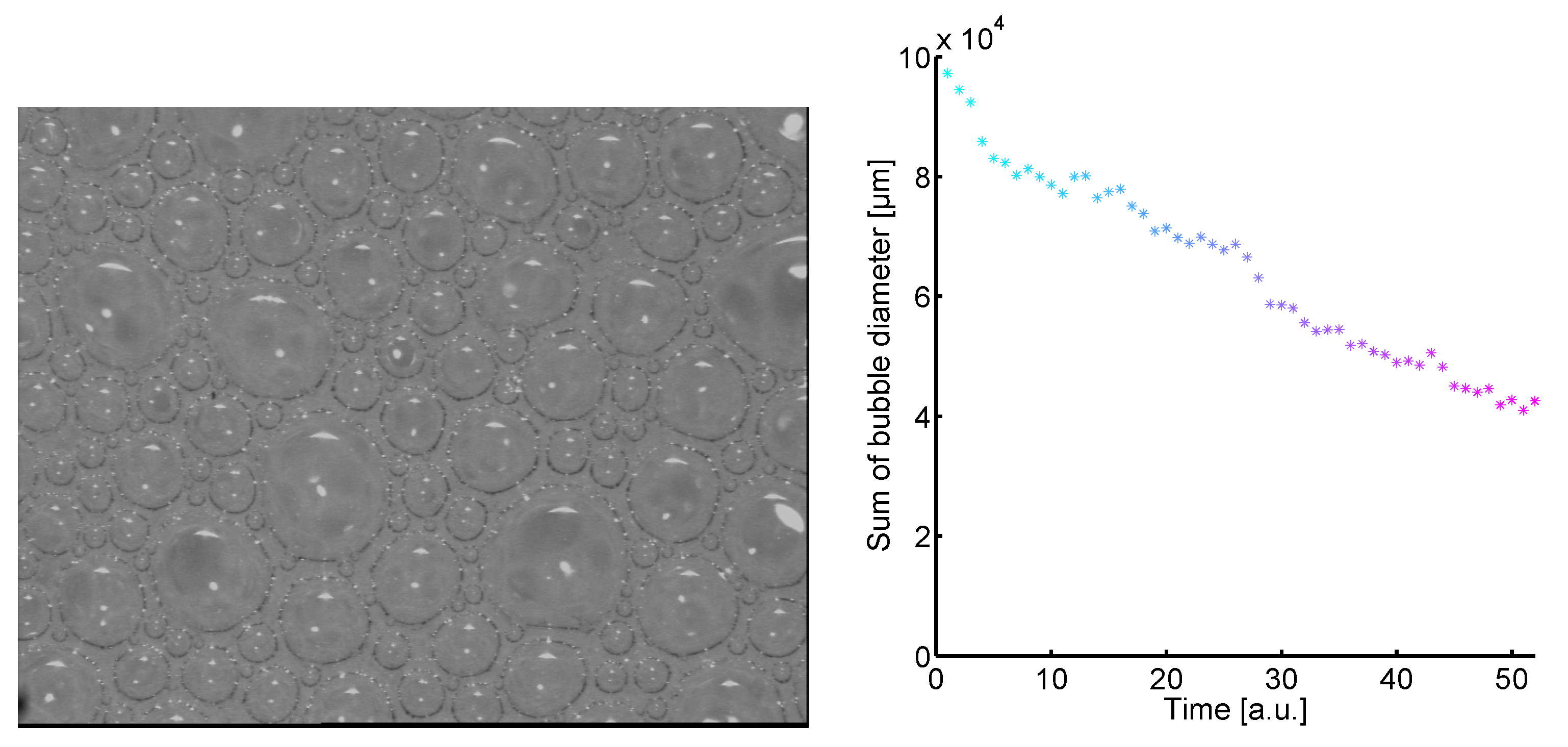
A rectangular glass vessel was filled with 20 mL of frothless beer (for this investigation Haake Beck beer was used) at a temperature of 24 ± 1C. By ultrasound treatment (Ultrasonik 28x; NEY) the beer was frothed up. A CV-M10 CCD-camera with a telecentric lens registered the bubbles at the 22 mL mark of the rectangular glass vessel. For illumination, a cold light source KL 2500 LC was used. Images were taken in five-second intervals. The size of the recorded image area was . Such an image is shown on the left in Figure 2.
Figure 2.
Left: Bubble image. Right: By smoothly varying from cyan to magenta the time development of the sum of the bubble diameters is shown.
Figure 2.
Left: Bubble image. Right: By smoothly varying from cyan to magenta the time development of the sum of the bubble diameters is shown.

Number of bubbles n and their sizes (diameter) of 52 images were determined. Then each image is defined by a size vector . Since the number of bubbles n decreases in time [12,14], the size vectors are defined by where n is the maximum number of bubbles given by the first size vector and subsequent size vectors are are filled with zeros. In other words the number of bubbles is held constant but the loss of bubbles is taken into account by allowing the size zero. Note that the normalization of the individuals introduced by Lorenz (Section 2.1.) is not applied. Originally, the concept of Lorenz curves were used to compare different populations and their income distributions without dynamics. Hence, the extension of the size vectors with zeros is necessary in order to take into account the loss and the size development of bubbles. Not only the number of bubbles decreases in time but also the sum of diameters have the tendency to decrease in time. In Figure 2 (right) the decrease of the sum of the bubble diameters is shown and illustrated by a smooth variation from cyan () to magenta ().
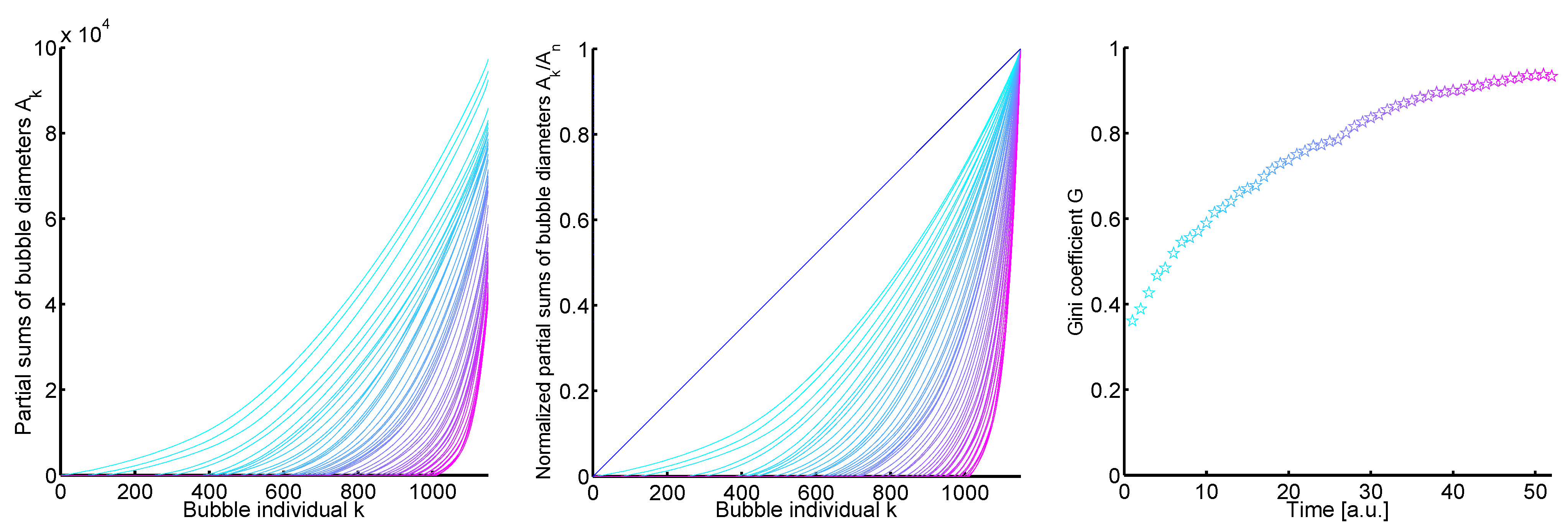
Firstly, the partial sum vectors of the increasingly sorted size vectors are generated. On the left in Figure 3 one sees the plot with , , and . The temporal development of these curves is illustrated again by the smoothly variation from cyan () to magenta ().
By normalizing the partial sum vectors in Figure 3 (left) the Lorenz curves are obtained. The plot is given by with , , and , see Figure 3 (middle). Additionally, a blue line is shown which gives the line of equality.
It seems for both plots in Figure 3 (left and middle) that each curve at lies below the curve at t which would mean that the development of the size vectors corresponds to a process which continuously develops away from equality (demixing process). But there are a few curves which cross. Despite the crossing curves, the temporal development of the Gini coefficient which gives the distance to the line of equality is monotonous, see Figure 3 (right).
In terms of Lorenz curves and Gini coefficient the temporal development of the bubble sizes can be characterized by a demixing process. It can be expected that the corresponding histograms of the raw data show a similar behaviour. Then the small image size does not enable a process separation to find; in order to prove this a linear scaling concerning the bubble size classes will be introduced in the following. Note that the demixing process of the bubble sizes described by Lorenz curves changes to a mixing process of bubble size histograms where bubble individuals are distributed over size classes.
Figure 3.
Left: The plot of the partial sum vectors of the increasingly sorted size vectors a. The plot is given by where k corresponds to the bubble individuals (), is the partial sum of the bubble diameters, and is set to zero. The temporal development is illustrated by the coloration of the curves from cyan () to magenta (). Middle: The Lorenz curves of the size vectors a. The plot is given by the bubble individuals and the normalized partial sum vectors of the increasingly sorted size vectors a, , with . The coloring gives the temporal development (cyan and magenta ). The line of equality is shown in blue. Right: The temporal development of the Gini coefficient G of the Lorenz curves (plot in the middle). The Gini coefficient increases monotonously in time.

3.2. Linear Scaling
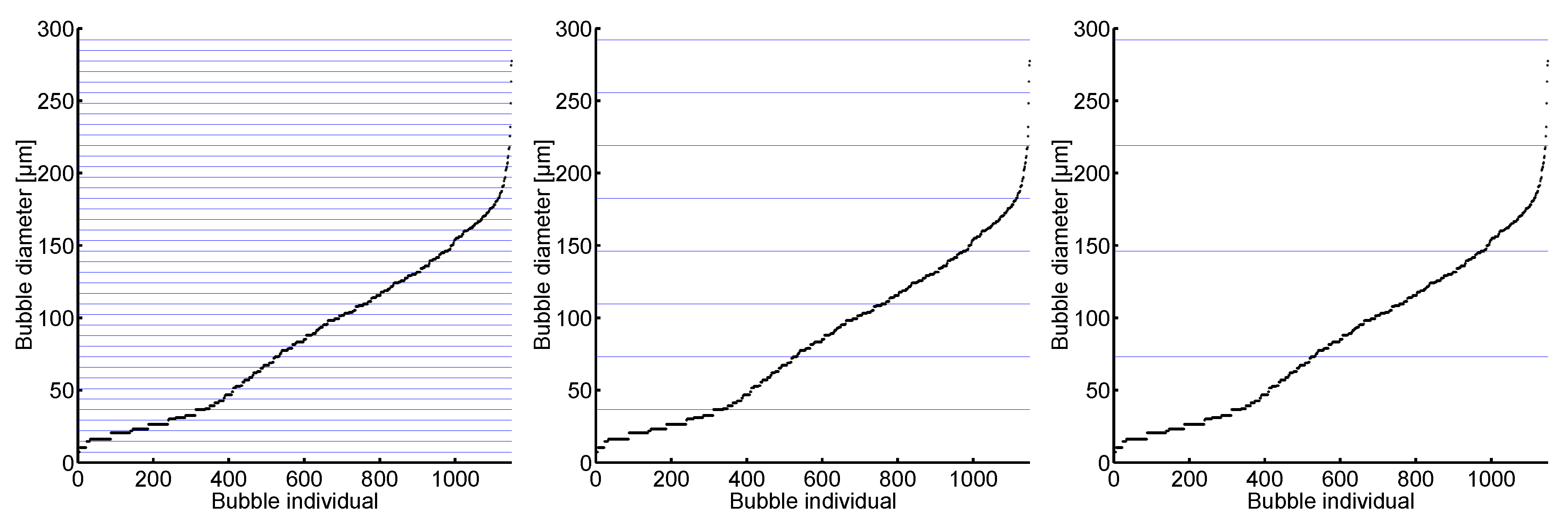
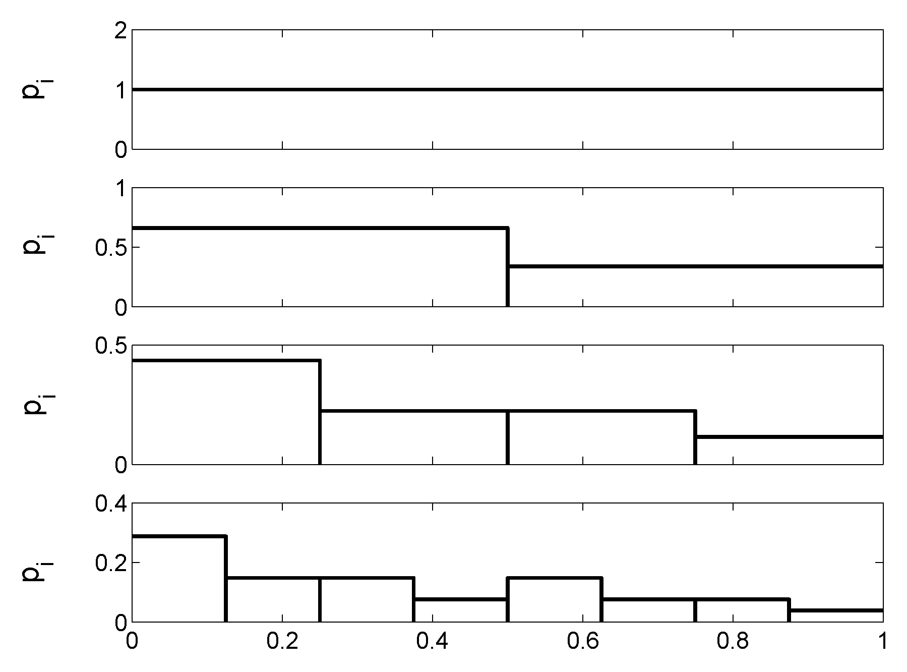
As reference, the initial bubble size vector with its smallest size, , is set. Then the classes are defined by the left-open and right-closed intervals with , where j is incremented until all bubble sizes are taken into account. The next step to reduce the number of size classes is to define the classes by multiples of . Then the classes are defined by the intervals where q is the multiplication or scaling factor which is incremented until all bubble sizes are in one class. This procedure can be illustrated by horizontal bars which depend on . In Figure 4 the increasingly sorted bubble sizes of the initial bubble size vector are shown with the size classification from left to right.
It is easy to see that for all bubbles of the initial bubble size vector belong to one class. More exactly, the minimum scaling factor of the first distribution in order to assign all sizes to one class is . The corresponding histograms of the classification in Figure 4 are given in Figure 5.
Figure 4.
The increasingly sorted bubble sizes of the initial bubble size vector . On the left the classification is formed by the multiples of with and; in the middle the classification is set by , , and on the right with , .
Figure 4.
The increasingly sorted bubble sizes of the initial bubble size vector . On the left the classification is formed by the multiples of with and; in the middle the classification is set by , , and on the right with , .

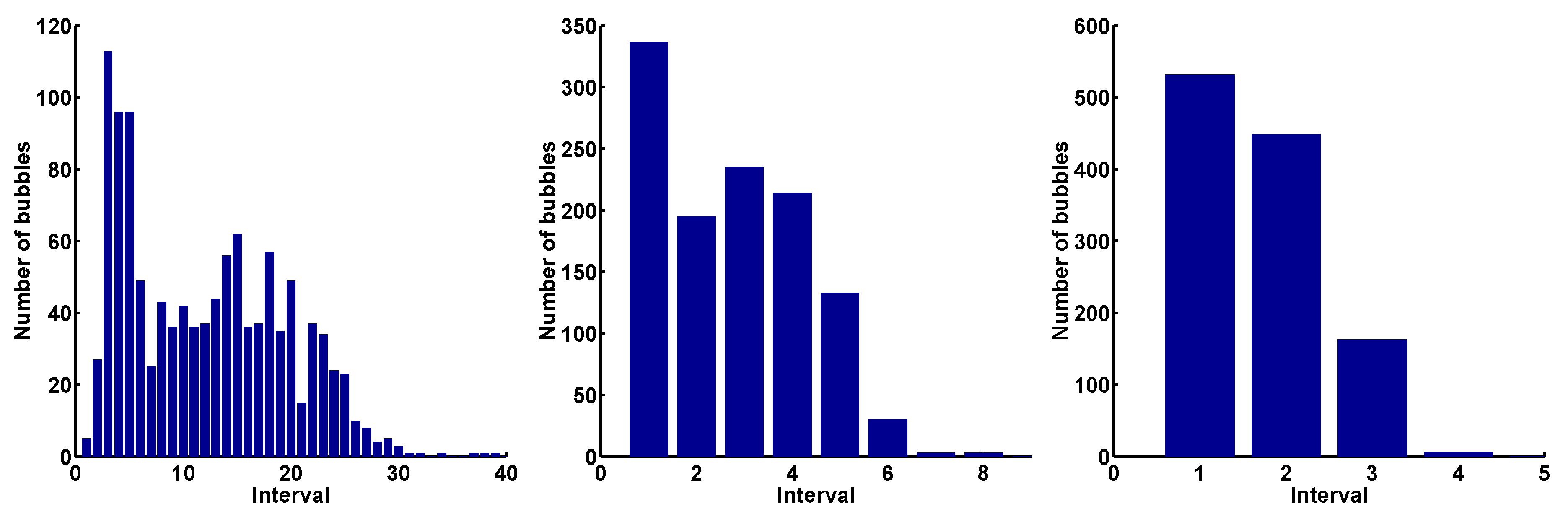
Figure 5.
The corresponding histograms of the classification of Figure 4. Left: ; middle: ; right: .
Figure 5.
The corresponding histograms of the classification of Figure 4. Left: ; middle: ; right: .

The characteristics of the histograms clearly change with increasing q. Particularly, the number of size classes (intervals) and the modality of the distributions are diminished from to . One may expect that there is a great loss of information by reducing the number of size classes which is accompanied by a decreasing modality. Of course, there will be no information, if the size classes are too large such that all sizes of all size vectors fall into one size class. Mapping the normalized histograms onto real values by the Shannon entropy (1) provides information about the underlying process of the temporal development of the histograms depending on q.
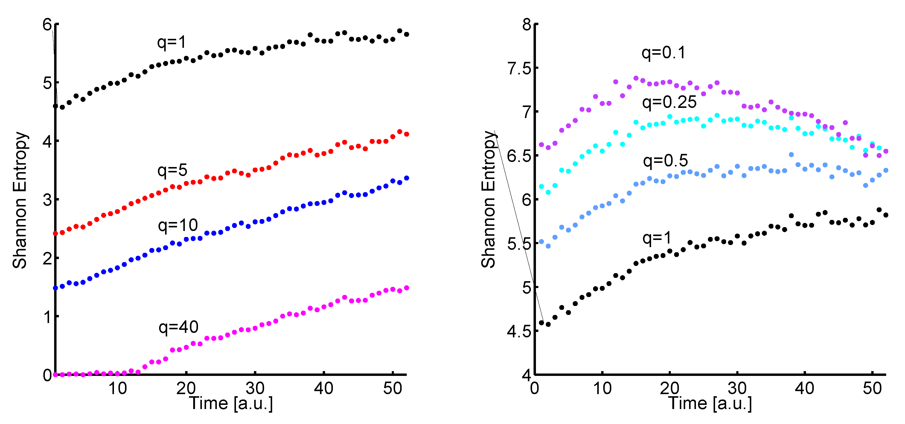
In Figure 6 (left) the time development of the Shannon entropy values of the histograms for (black plot), (red plot), (blue plot), and (magenta plot) is shown. The latter is a kind of limit since the size classes become too large and the histograms at the beginning are mapped onto zero by the Shannon entropy (1).
It is very interesting that the basic behaviour is preserved although the histograms are strongly reduced. The Shannon entropy values increase in tendency in time which corresponds to a mixing process. The next step is to use q values which are less than one.
Figure 6.
Left: The temporal development of the Shannon entropy (1) of the histograms for (black plot), (red plot), (blue plot), and (magenta plot). Right: The temporal development of the Shannon entropy (1) of the histograms for (black plot), (light blue plot), (cyan plot), and (mauve plot).
Figure 6.
Left: The temporal development of the Shannon entropy (1) of the histograms for (black plot), (red plot), (blue plot), and (magenta plot). Right: The temporal development of the Shannon entropy (1) of the histograms for (black plot), (light blue plot), (cyan plot), and (mauve plot).

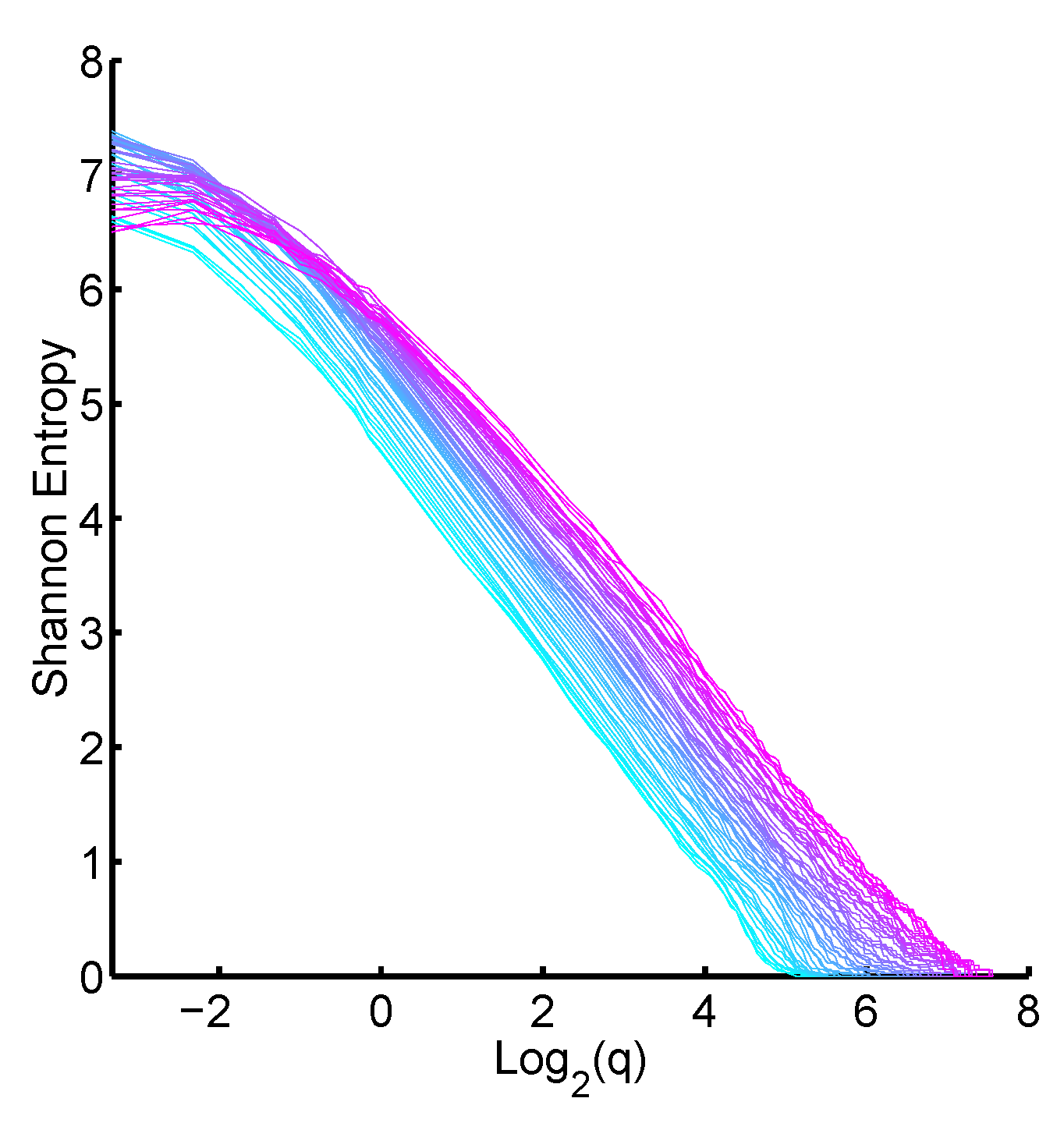
In Figure 6 (right) the temporal development of the Shannon entropy values of the histograms for as reference (black plot), (light blue plot), (cyan plot), and (mauve plot) is shown. With decreasing q the Shannon entropy plot changes considerably. Particularly for the mixing process becomes a demixing process after 15 time units. But setting is not recommended, since the corresponding bin width is very small (a tenth of the smallest bubble size of the initial distribution). Hence, there is a further restriction for small q. The limits of q can be illustrated by plotting where are the relative frequencies of the normalized histograms. The mixing process of the normalized histograms is preserved for a linear behaviour of the plot or if , see Figure 7. The time dependence of the histograms is given by smoothly varying from cyan to magenta.
Figure 7.
Development of the Shannon entropy of the histograms depending on the logarithmus dualis of the scaling factor q, . One sees that for a certain section the value of remains constant. The coloration of the plot gives the time dependence as before.
Figure 7.
Development of the Shannon entropy of the histograms depending on the logarithmus dualis of the scaling factor q, . One sees that for a certain section the value of remains constant. The coloration of the plot gives the time dependence as before.

Particularly, for q values between 8 and 16 () the slope for all distributions is approximately the same. These q values are the best selection for the size classification.
As expected the demixing process of Lorenz curves is mapped onto a mixing process of histograms for all size classifications with . A process separation of drainage and ageing as in [11] cannot be found, but a region for best size classification is suggested and can be defined by a common slope, see Figure 7. Consequently, a statistical process separation only occurs for sufficiently large foam images.
4. Dimensions
From the plot in Figure 7 new characteristics of bubble size distributions can be derived. The Rényi entropy of order f [20]
gives in the limiting case for of the Shannon entropy, . N represents the number of occupied classes. For one obtains (logarithm of the cardinality of p) and (correlation entropy). The plot of these entropies depending on different scales gives the so-called Rényi dimensions [21]:
where s is the scaling factor. Classically, for one obtains the capacity (fractal or Hausdorff dimension [22]), the information, and the correlation dimension:
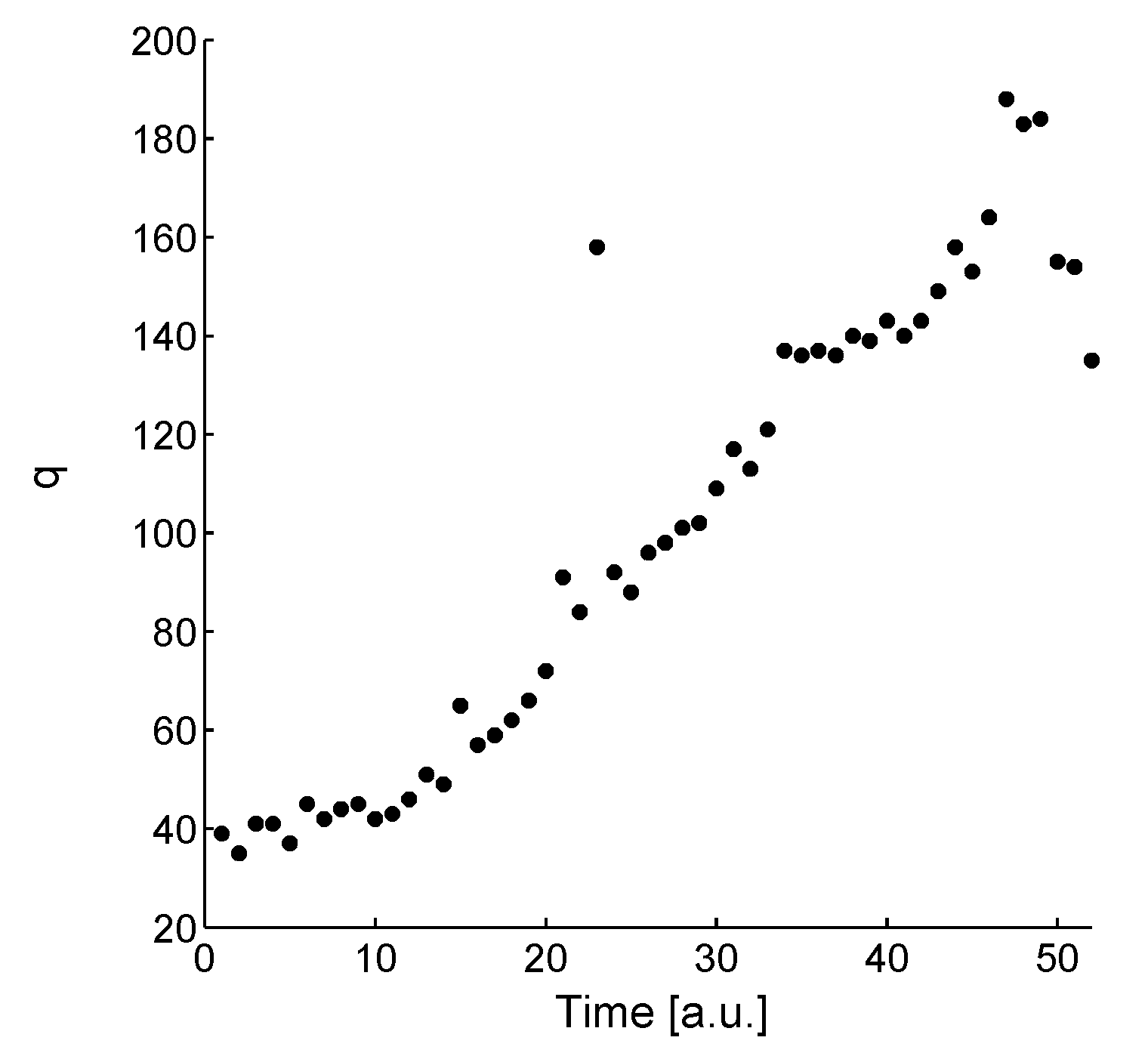
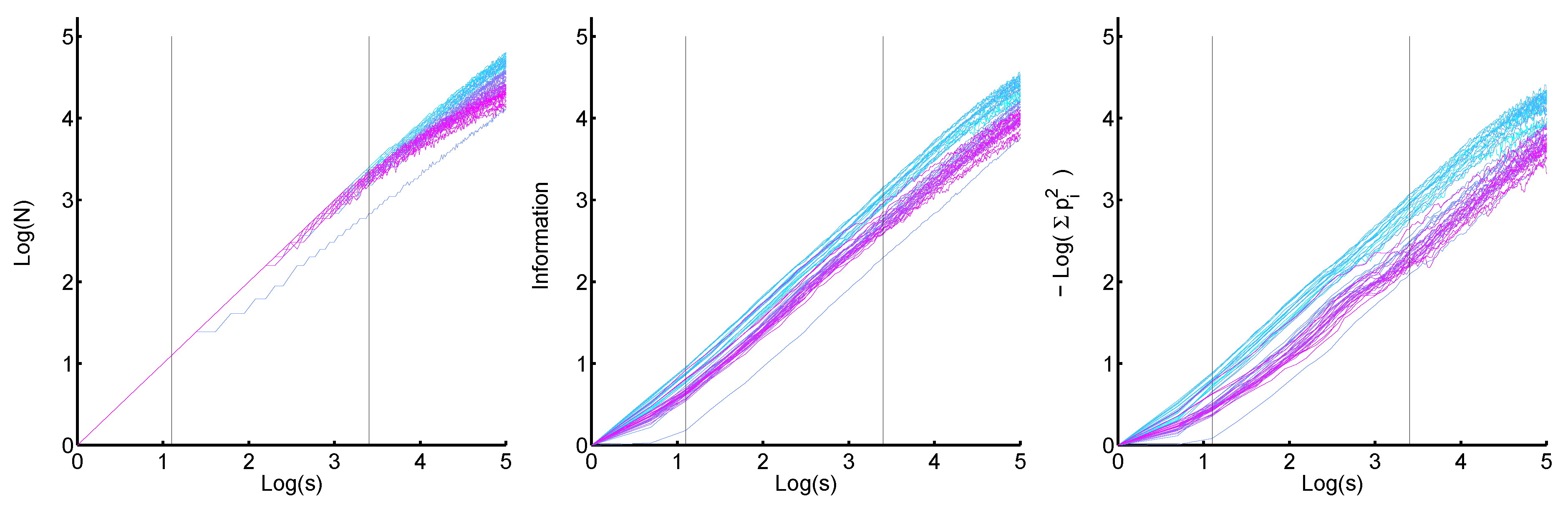
For the number of occupied size classes N depending on s is considered. is comparable to the plot in Figure 7. The sum gives the probability that two bubbles are in the same size class. The scaling factor s is defined by: , where the braces indicate the ceiling function. Then the dimensions are generated over the individual data scale of each bubble size distribution. Additionally, the ceiling function is used in order to define a minimum integer value of q as starting point which becomes systematically reduced by the factor s. For example, the first bubble size distribution has the minimum integer value where all sizes fall into one size class (see section 3.2.). The second step, , leads to a q value of which defines the size class and so on. The minimum integer q of the second distribution is 35 for instance. The temporal development of these minimum integer q factors have the tendency to increase, this is shown in Figure 8.
The plots , , and for all bubble size distributions are given in Figure 9 from left to right. For the mean values and their standard deviations of the dimensions are with , with , and with .
In the beginning, the capacity dimension equals one, which means that with each size reduction of the classes all resulting classes are occupied. For further reductions, this dimension deviates from one which indicates an increase of multimodality. As above mentioned the information dimension gives the gain of information with shrinking size classes. In Figure 7 the loss of information is considered with another scale (). The high value of the information dimension indicates that with each reduction of the size classes the relative frequencies of these classes are more mixed. This and the meaning of the value of the correlation dimension will be discussed in the following section.
Figure 8.
The temporal development of the minimum integer q factor of the bubble size distributions.
Figure 8.
The temporal development of the minimum integer q factor of the bubble size distributions.

Figure 9.
Left: The number of occupied classes (positive frequencies) is plotted against the factor , where ; the mean value of the fractal dimension is with standard deviation . Middle: The plot for the information dimension, with . Right: The plot , where and . The 23rd distribution is a maverick and is omitted for computing the fractal dimension. The dimensions are defined in the interval , black lines.
5. Discussion
For this statistical investigation it is assumed that the development of the bubble sizes is a deterministic process. The initial bubble size distribution determines successive distributions. Hence, size classes are defined on the basis of the first distribution. Additionally, the chosen size classes are equal and closed over the data set contrary to former investigations [7,8,9,10,11,12,13,14,15] where the last size class was open. In the literature several recipes for the computation of the number of size classes and their sizes can be found [23,24,25]. But these approaches are either not directly applicable to dynamical systems or already included in this here introduced systematic data binning.
It is surprising that no specific size classification for the optimal evaluation of the foam experiment exists but size limits of size classes can be defined. In Figure 7 one sees that there is a region where with increasing (the size classes become larger) the loss of information is approximately constant for all distributions. Although salient features of the bubble size histograms vanish with increasing scaling factor q (compare to Figure 5) the temporal development of the Shannon entropy values of the histograms is preserved for a certain region, Figure 6 (left). As reference for the temporal development of the Shannon entropy values the Lorenz curves which are mapped onto the Gini coefficient are used. This concept uses the original data without a classification.
The Rényi dimensions of the bubble size distributions for decrease, , which indicates that the distributions are multifractal [26]. But which insights are gained by this characteristic? Considering the construction of a self-similar distribution by iterated bisecting [27] it can be assumed that the resulting structure can be partially found in the bubble size distributions. If for each bisecting the resulting proportions are for one size class and for the other one, see Figure 10, the dimensions will be , , . These values are entirely comparable to the dimensions of the bubble size distributions. Especially, the information and the correlation dimension practically coincide within experimental accuracy ( and ).
Of course, the bubble size distributions do not obey exactly this construction but it can be supposed that the bubble size distributions are self-similar in certain regions.
Figure 10.
Construction of a self-similar distribution by iterated bisecting with . From top to bottom the scaling factor is . The corresponding Rényi dimensions are , , .
Figure 10.
Construction of a self-similar distribution by iterated bisecting with . From top to bottom the scaling factor is . The corresponding Rényi dimensions are , , .

The construction of the distributions in Figure 10 and the value of the information dimension of the bubble size distributions indicate that the differences of the increasingly sorted bubble sizes are quite small. Hence, each size class reduction leads to relative frequencies which are more mixed. For less mixed relative frequencies the information and correlation dimension become smaller. The dimensions become one for which leads to equal distributions. The small differences of the bubble sizes also cause the relatively high value of the correlation dimension. The larger the value of the correlation dimension the larger the probability that two bubbles are in the same size class. Since the foam system is small—the number of bubble individuals ranges in time from 1150 to 139—higher Rényi dimensions which correspond to the probability of f-tuples () of bubbles with marginally differing sizes are omitted. It would be interesting to investigate larger foam systems in order to generate a sufficiently large multifractal spectrum for the determination of the Lipshitz-Hölder mass exponent [26]. Moreover, large foam systems including process separation are ought to be investigated in order to prove the general applicability of the above-mentioned concepts to bubble size distributions.
6. Conclusions
Both Lorenz curves and systematic data binning of bubble size distributions do not show a statistical process separation of drainage and ageing of the presented foam measurement. Consequently, a sufficiently large foam image size is required to divide the bubble size development into drainage and ageing. The systematic data binning leads to an approach of an optimal bin width selection. Moreover, Rényi dimensions can be calculated and indicate multifractality of bubble size distributions. By means of a simple bisecting model it can be assumed that bubble size distributions are partially self-similar. Both Rényi dimensions and self-similarity point out that the distribution structure is preserved during the whole bubble size development. Only the size range of the distributions changes in time. This range is described by the q factor where the scaling factor s is one.
Acknowledgements
I am indebted to Markus Eiswirth and Peter Plath for many fruitful discussions and their generous support. Both are very distinguished scientists who have taught me to see things in an unusual scientific way. I deem myself lucky for having worked together with them.
References
- Hardy, P.G.H.; Littlewood, J.E.; Pólya, G. Inequalities; Cambridge University Press: London, UK, 1934. [Google Scholar]
- Muirhead, R.F. Some Methods Applicable to Identities and Inequalities of Symmetric Algebraic Functions of N Letters. Proc. Edinburgh Math. Soc. 1903, 21, 144–157. [Google Scholar] [CrossRef]
- Alberti, P.M.; Uhlmann, A. Dissipative Motion in State Spaces; Teubner Texte zur Mathematik Band 33; Teubner-Verlag: Leipzig, Germany, 1981. [Google Scholar]
- Alberti, P.M.; Uhlmann, A. Stochasticity and partial order: doubly stochastic maps and unitary mixing; Dordrecht: Boston, MA, USA, 1982. [Google Scholar]
- Marshall, A.W.; Olkin, I. Inequalities: Theory of Majorization and Its Applications; Academic Press: New York, NY, USA, 1979. [Google Scholar]
- Arnold, B.C. Majorization: Here, There and Everywhere. Stat. Sci. 2007, 22, 407–413. [Google Scholar] [CrossRef]
- Sauerbrei, S.; Plath, P.J. Apollonische Umordnung des Schaums. Brauindustrie 2004, 89, 20–23. [Google Scholar]
- Sauerbrei, S. Mathematics of Foam Decay. PhD thesis, University of Bremen, Germany, 2005. [Google Scholar]
- Sauerbrei, S.; Haß, E.C.; Plath, P.J. The Apollonian Decay of Beer Foam–Bubble Size Distribution and the Lattices of Young Diagrams and Their Correlated Mixing Functions. Discrete Dyn. Nat. Soc. 2006, 1–35. [Google Scholar] [CrossRef]
- Sauerbrei, S.; Sydow, U.; Plath, P.J. On the Characterization of Foam Decay with Diagram Lattices and Majorization. Z. Naturforsch. 2006, 61a, 153–165. [Google Scholar] [CrossRef]
- Sauerbrei, S.; Plath, P.J. Diffusion Without Constraints. J. Math. Chem. 2007, 42, 153–175. [Google Scholar] [CrossRef]
- Sauerbrei, S.; Knicker, K.; Haß, E.C.; Plath, P.J. Weak Majorization as an Approach to Non-Equilibrium Foam Decay. Appl. Math. Sci. 2007, 1, 527–550. [Google Scholar]
- Sauerbrei, S.; Knicker, K.; Haß, E.C.; Plath, P.J. Eine Mathematische Beschreibung des Schaumzerfalls. Leibniz Online 2007, 3, 1863–3285. [Google Scholar]
- Sauerbrei, S.; Plath, P.J.; Eiswirth, M. Discrete Dynamics by Different Concepts of Majorization. Int. J. Math. Math. Sci. 2008, 2008, 474782:1–474782:21. [Google Scholar] [CrossRef]
- Sauerbrei, S.; Knicker, K.; Sydow, U.; Haß, E.C.; Plath, P.J. An Overview of the Dynamics of Bubble Size Distributions of a Beer Foam Decay and their Order Structure. In Vernetzte Wissenschaften–Crosslinks in Natural and Social Sciences; Plath, P.J., Haß, E.C., Eds.; Logos Verlag: Berlin, Germany, 2008; pp. 291–304. [Google Scholar]
- Shannon, C.E. A Mathematical Theory of Communication. AT&T Tech. J. 1948, 27, 379–423, 623–656. [Google Scholar]
- Lorenz, M.O. Methods of measuring concentration of wealth. J. Amer. Statist. Assoc. 1905, 9, 209–219. [Google Scholar] [CrossRef]
- Dalton, H. The measurement of the inequality of income. Econom. J. 1920, 30, 34–361. [Google Scholar] [CrossRef]
- Gini, C. Variabilità e mutabilità (1912). In Memorie di metodologia statistica; Pizetti, E., Salvemini, T., Eds.; Libreria Eredi Virgilio Veschi: Rome, Italy, 1955. [Google Scholar]
- Rényi, A. On Measures of Entropy and Information. In Proceedings of the Fourth Berkeley Symposium on Mathematical Statistics and Probability; Neyman, J., Ed.; Univerisity of California Press: Berkeley, CA, USA, 1961; Volume 1, pp. 547–561. [Google Scholar]
- Rényi, A. Wahrscheinlichkeitsrechnung, mit einem Anhang über Informationstheorie, 5th ed.; Deutscher Verlag der Wissenschaften: Berlin, Germany, 1977. [Google Scholar]
- Mandelbrot, B.B. The Fractal Geometry of Nature; W.H. Freeman and Company: New York, NY, USA, 1983. [Google Scholar]
- Sturges, H.A. The choice of a class interval. J. Am. Stat. Assoc. 1926, 21, 65–66. [Google Scholar] [CrossRef]
- Scott, D.W. On optimal and data-based histograms. Biometrika 1979, 66, 605–610. [Google Scholar] [CrossRef]
- Freedman, D.; Diaconis, P. On the histogram as a density estimator: L2 theory. Z. Wahrscheinlichkeit. 1981, 57, 453–476. [Google Scholar] [CrossRef]
- Schroeder, M. Fractals, Chaos, Power Laws; W.H. Freeman and Company: New York, NY, USA, 1991. [Google Scholar]
- Pietronero, L.; Siebesma, A.P. Self-similarity of fluctuations in random multiplicative processes. Phys. Rev. Lett. 1986, 57, 1098–1101. [Google Scholar] [CrossRef] [PubMed]
© 2010 by the author; licensee Molecular Diversity Preservation International, Basel, Switzerland. This article is an open-access article distributed under the terms and conditions of the Creative Commons Attribution license http://creativecommons.org/licenses/by/3.0/.
Share and Cite
MDPI and ACS Style
Sauerbrei, S. Lorenz Curves, Size Classification, and Dimensions of Bubble Size Distributions. Entropy 2010, 12, 1-13. https://doi.org/10.3390/e12010001
AMA Style
Sauerbrei S. Lorenz Curves, Size Classification, and Dimensions of Bubble Size Distributions. Entropy. 2010; 12(1):1-13. https://doi.org/10.3390/e12010001
Chicago/Turabian StyleSauerbrei, Sonja. 2010. "Lorenz Curves, Size Classification, and Dimensions of Bubble Size Distributions" Entropy 12, no. 1: 1-13. https://doi.org/10.3390/e12010001