Forecasting the Stock Market with Linguistic Rules Generated from the Minimize Entropy Principle and the Cumulative Probability Distribution Approaches

Abstract

To forecast a complex and non-linear system, such as a stock market, advanced artificial intelligence algorithms, like neural networks (NNs) and genetic algorithms (GAs) have been proposed as new approaches. However, for the average stock investor, two major disadvantages are argued against these advanced algorithms: (1) the rules generated by NNs and GAs are difficult to apply in investment decisions; and (2) the time complexity of the algorithms to produce forecasting outcomes is very high. Therefore, to provide understandable rules for investors and to reduce the time complexity of forecasting algorithms, this paper proposes a novel model for the forecasting process, which combines two granulating methods (the minimize entropy principle approach and the cumulative probability distribution approach) and a rough set algorithm. The model verification demonstrates that the proposed model surpasses the three listed conventional fuzzy time-series models and a multiple regression model (MLR) in forecast accuracy.

1. Introduction

Individual stock investors never stop dreaming of becoming wealthy by trading stocks. However, only a very few people can make huge profits because it is enormously difficult to accurately predict stock prices on a daily basis. In the stock market, there are too many factors influencing prices, such as stock news, company financial reports and government economic policies. Therefore, since the first stock market opened, many analytical methods and forecasting models have been advanced in an attempt to land the big fish in the stock market sea. Two major stock market analysis approaches, fundamental and technical analysis [1,2,3,4], are commonly used by both stock analysts and artificial intelligence (AI) methods proposed by the researchers who are interested in stock markets [5,6,7,8,9,10].

Technical analysis is a subjective way to predict stock market fluctuations, although, more hidden information for future prices is given from technical indicators, which are transformed from basic indexes by specific mathematic equations [2,11], than is given by daily basic indexes (time, open index, high index, low index, close index and volume). Two analysts can come up with two completely different forecasts from the same analytical charts and technical indicators. Much of technical analysis is truly “in the eye of the beholder [4]”. Therefore, viewed from the investor’s point of view, empirical rules or investment experience are necessary in order to predict stock prices accurately.

However, with the emergence of data mining techniques, more and more AI tools have been applied in predicting stock markets, such as choosing an optimal portfolio by genetic algorithms [5], selecting real-world stocks by neural networks [12], and predicting the S&P 100 index by rough sets [13]. In this paper, in order to avoid any possible intrusions of the model designer’s subjective predictions, based on technical analytical methods, one objective, automatic, artificial intelligence model is proposed, which combines three data mining techniques into forecasting processes: (1) MEPA (minimize entropy principle approach), which subdivides data into membership functions [14,15,16,17,18]; (2) CPDA (cumulative probability distribution approach), which fuzzifies the observations into linguistic values based on the cumulative probability of the observations [17,19,20]; and (3) rough set theory [17,19,21,22,23,24], which mines rules from the linguistic dataset. Using these techniques, objective and effective rules can be produced as the basis for forecasting.

2. Related Works

This section briefly reviews the related literature, including the minimize entropy principle approach (MEPA), the cumulative probability distribution approach (CPDA), rough set theory, and defuzzification methods.

2.1. The Minimize Entropy Principle Approach (MEPA)

A key goal of entropy minimization analysis is to determine the quantity of information in a given dataset. The entropy of a probability distribution is a measure of the uncertainty of the distribution [15]. To subdivide the data into membership functions, establishing the threshold between classes of data is needed. A threshold line can be determined with an entropy minimization screening method, after which the segmentation process may begin, with the initial segmentation divided into two classes. Therefore, a repeated partitioning with threshold value calculations will allow us to partition the data set into a number of fuzzy sets [25].

Assume that a threshold value is being sought for a sample in the range between x₁ and x₂. An entropy equation is written for the regions [x₁, x] and [x, x₂], with the first region denoted p and the second region denoted q. An entropy [14,16] with each value of x is expressed by following equations (1) through (3):

$$S(x)=p(x)S_p(x)+q(x)S_q(x)$$

(1)

where:

$$S_p(x)=-[p_1(x)\ln p_1(x)+p_2(x)\ln p_2(x)]$$

(2)

$$S_q(x)=-[q_1(x)\ln q_1(x)+q_2(x)\ln q_2(x)]$$

(3)

where p_k(x) and q_k(x) = conditional probabilities (see equation (4)) that the class k sample is in the region [x₁, x₁+x] and [x₁+x, x₂], respectively; p(x) and q(x) = probabilities that all samples are in the region [x₁, x₁+x] and [x₁+x, x₂], respectively:

$$p(x)+q(x)=1$$

(4)

A value of x that gives the minimum entropy is the optimum threshold value. The entropy [14,16] estimates of p_k(x) and q_k(x), p(x) and q(x), are calculated by following equation (5) to equation (8):

$$p_k(x)=\frac{n_k(x)+1}{n(x)+1}$$

(5)

$$q_k(x)=\frac{N_k(x)+1}{N(x)+1}$$

(6)

$$p(x)=\frac{n(x)}{n}$$

(7)

$$q(x)=1-p(x)$$

(8)

where:

• n_k(x) = number of class k samples located in [x₁, x₁+x];
• n(x) = the total number of samples located in [x₁, x₁+x];
• N_k(x) = number of class k samples located in [x₁+x, x₂];
• N(x) = the total number of samples located in [x₁+x, x₂];
  n = total number of samples in [x₁, x₂].

Figure 1 shows partitioning processes for MEPA. While moving x in the region [x₁, x₂], we calculate the values of entropy for each position of x. The value of x in the region that holds the minimum entropy is called the primary threshold (PRI) value.

Figure 1. Partitioning process of minimize entropy principle approach.

Figure 1. Partitioning process of minimize entropy principle approach.

2.3. The Cumulative Probability Distribution Approach (CPDA)

The cumulative probability of normal distribution can be used to define intervals of linguistic value [17,19,26]. The procedures of cumulative probability distribution approach are described in four steps, as follows:

Step 1: Test normal distribution. In this step, CDPA is used to ascertain whether the target dataset follows normal distribution. The Lilliefors test [27] is used to identify the distribution characteristic of the observations contained in the dataset.

Step 2: Define the universe of discourse U. Define the universe of discourse, U, as [D_min − σ, D_max + σ] for the target dataset, where D_min denotes the minimum value; D_max denotes the maximum value; and σ denotes the standard deviation for the observations contained in the target dataset.

Step 3: Determine interval length and build membership function. There are three sub-steps in this process: (1) define the lower bound of cumulative probability (P_LB), and the upper bound of cumulative probability (P_UB); (2) invert the normal cumulative distribution function (CDF) for defined linguistic values; and (3) define fuzzy sets and build membership functions.

Step 3–1: Define lower bound and upper bound of cumulative probability. For each given linguistic value, the lower bound of cumulative probability (P_LB) and the upper bound of cumulative probability (P_UB) are defined by equations (9) through (10) [28]:

$$P_{LB}^1=1-{\displaystyle \sum _{i=2}^n{P}_{LB}^i}$$

(9)

P ⁱ_LB = (2i – 3) / 2n, (2 ≦ i ≦ n)

P_UB = i / n, (1 ≦ i ≦ n)

(10)

where i denotes the order of the linguistic value and n denotes the amount for defined linguistic values.

Based on equation (9) to (10), the lower and upper bounds with cumulative probability for five linguistic values are listed in Table 1.

Table 1. Lower and upper bound of cumulative probability for linguistic value.

Linguistic Value	Cumulative Probability
	PLB	PUB
L1	0	0.2
L2	0.2	0.4
L3	0.4	0.6
L4	0.6	0.8
L5	0.8	1

Table 1. Lower and upper bound of cumulative probability for linguistic value.

Linguistic Value	Cumulative Probability
	PLB	PUB
L1	0	0.2
L2	0.2	0.4
L3	0.4	0.6
L4	0.6	0.8
L5	0.8	1

Step 3–2: Inverting the normal cumulative distribution function for defined linguistic values. To produce linguistic intervals for each linguistic value, the normal cumulative distribution function (CDF), defined by equation (11) [29], is given:

$$P=F(x|u,\sigma )=\frac{1}{\sigma \sqrt{2\pi }}{\displaystyle {\int }_{-\infty }^x{e}^{\frac{-{(t-u)}^2}{2{\sigma }^2}}dt}$$

(11)

where P denotes the probability that a single observation from a normal distribution with parameters µ and σ will fall in the interval (−∞ x].

From an algorithm for computing the inverse normal cumulative distribution function [30], the lower and upper bound for five linguistic values can be produced. Table 2 demonstrates the five sets of linguistic intervals (lower and upper bound values) for five linguistic values of price fluctuation in the 2001 TAIEX, based on the lower bound (P_LB) and upper bound (P_UB) of cumulative probability from Table 1.

Table 2. Linguistic intervals for five linguistic values of price fluctuation.

Linguistic Value	Linguistic Interval
	PLB	PUB
L1	−560.2145	−86.3797
L2	−126.9697	−32.1029
L3	−57.1115	14.647
L4	−8.728	68.9238
L5	39.6556	658.5045

Table 2. Linguistic intervals for five linguistic values of price fluctuation.

Linguistic Value	Linguistic Interval
	PLB	PUB
L1	−560.2145	−86.3797
L2	−126.9697	−32.1029
L3	−57.1115	14.647
L4	−8.728	68.9238
L5	39.6556	658.5045

Step 3–3: Define fuzzy sets and build membership functions. The triangle fuzzy number (TFN) [31] is used to present the fuzzy sets for the linguistic variables of the price fluctuations (A1 to A5) based on the linguistic intervals from Table 4. The membership function of the TFN is defined as equation (12).

$${\mu }_{{\tilde{A}}_i}(x)=\{\begin{array}{c}\begin{array}{c}\begin{array}{cc}0,& x<a\end{array}\end{array}\\ \begin{array}{cc}\frac{x-a}{b-a},& a\le x<b\end{array}\\ \begin{array}{c}\begin{array}{cc}\frac{c-x}{c-b},& b\le x<c\end{array}\end{array}\\ \begin{array}{cc}0,& x\ge c\end{array}\end{array}$$

(12)

where ${\mu }_{{\tilde{A}}_i}(x)$ denotes the membership value of crisp data x belonging to fuzzy set ${\tilde{A}}_i$; the lower bound, midpoint and upper bound of ${\tilde{A}}_i$ are defined by a, b and c, respectively.

If an observation meets two or more membership functions, the linguistic value with the maximum membership value is chosen and labeled on the observation. Table 3 demonstrates the parameterized triangle fuzzy numbers for linguistic variables of the price fluctuations (L1 to L5) from Table 2.

Table 3. Parameterized fuzzy numbers for price fluctuations of the 2001 TAIEX.

Linguistic Value	Triangular Fuzzy Number(a, b, c)
	a(lower bound)	b(midpoint)	c(upper bound)
L1	−560.2145	−323.297	−86.3797
L2	−126.9697	−79.5363	−32.1029
L3	−57.1115	−21.2323	14.647
L4	−8.728	30.0979	68.9238
L5	39.6556	349.08	658.5045
Standard Derivation = 92.26; Mean = −8.73

Table 3. Parameterized fuzzy numbers for price fluctuations of the 2001 TAIEX.

Linguistic Value	Triangular Fuzzy Number(a, b, c)
	a(lower bound)	b(midpoint)	c(upper bound)
L1	−560.2145	−323.297	−86.3797
L2	−126.9697	−79.5363	−32.1029
L3	−57.1115	−21.2323	14.647
L4	−8.728	30.0979	68.9238
L5	39.6556	349.08	658.5045
Standard Derivation = 92.26; Mean = −8.73

Step 4: Fuzzify the historical data. With the inverse of normal CDF and parameterized triangle fuzzy numbers for linguistic variables of price fluctuations, all observations contained in the target set can be fuzzifed as linguistic values.

2.4. Rough Set Theory

Rough set theory was proposed by Pawlak [21] in order to distill the rules that determine the safety performance of construction firms. Since the development of the original exposition of the rough set theory (RST) as a method of set approximation, it has continued to flourish as a tool for data mining [17,22,23,24].

Rough set theory is also a mathematical framework that deals with vagueness and uncertainty, and can be situated within the fields of artificial intelligence (AI), knowledge discovery in databases and data mining (DM). The rough set philosophy is founded on the assumption that with every object of the universe of discourse associated with it, some informational objects, characterized by the same information, are indiscernible in view of the available information about them. Any set composed of all indiscernible objects is called an elementary set and forms a basic granule of knowledge about the universe. Any union of elementary sets is referred to as a precise set, otherwise the set is rough.

A pair of precise sets, called the lower and the upper approximation of the rough set, is associated [21,32] with any rough set. The lower approximation consists of all objects which surely belong to the set, and the upper approximation contains all objects which possibly belong to the set. The difference between the upper and the lower approximation constitutes the boundary region of the rough sets. Approximations are two basic operations in the rough set theory. The basic notions in rough sets are shown in Figure 2 [19,33].

Figure 2. Basic notions for rough sets.

Figure 2. Basic notions for rough sets.

The rough set method is a series of logical reasoning procedures, used for analyzing an information system. An information system can be seen as a decision table, denoted by $S=(U,A,C,D)$, where U is universe of discourse, A is a set of primitive features, and $C,D\subset A$ are two subsets of features, assuming that $A=C\cup D$ and $C\cap D=\varnothing$, where C is called condition attribute, and D, as decision attribute.

An example of an accident occurrence decision table [34] is illustrated in Table 4. In it, five cases are characterized with three condition attributes: driver’s age, vehicle type and climate; and one decision attribute: accident type. The three condition attributes form four elementary sets $\{1,3\}$, $\left\{2\right\}$, $\left\{4\right\}$ and $\left\{5\right\}$. This means that cases, 1 and 3, are indiscernible, while the other cases are characterized uniquely with all available information. Therefore, the off-road accident type is described with the lower approximation set as $\left\{2\right\}$, and the upper approximation set as $\{1,2,3\}$. Similarly, the concept of the rollover accident type is characterized by its lower approximation set as $\{4,5\}$ and upper approximation set as $\{1,3,4,5\}$ [34], which generates rule and weight for better forecasting results.

Table 4. Accident cases with describing features.

Case	Driver’s Age	Vehicle Type	Climate	Accident Type
1	Young	motorcycle	sunny	Off-road
2	Old	automobile	sunny	Off-road
3	young	motorcycle	sunny	rollover
4	Middle-aged	motorcycle	sunny	rollover
5	Middle-aged	automobile	rainy	rollover

Table 4. Accident cases with describing features.

Case	Driver’s Age	Vehicle Type	Climate	Accident Type
1	Young	motorcycle	sunny	Off-road
2	Old	automobile	sunny	Off-road
3	young	motorcycle	sunny	rollover
4	Middle-aged	motorcycle	sunny	rollover
5	Middle-aged	automobile	rainy	rollover

2.5. Defuzzification

Defuzzification is the conversion of a practice quantity to a fuzzy quantity. Many defuzzification methods have been proposed and have become popular in defuzzifying fuzzy output functions. Four of these methods are summarized, as follows [25]:

Max-membership principle: this scheme is limited to the peak output function; it is given as the algebraic expression (13):

$$u_c(z^{*})\ge u_c(z)for\text{\hspace{0.17em}}allz\in Z$$

(13)

Centroid method: this procedure (also called center of area, center of gravity) is the most popular defuzzification method; it is given as the algebraic expression (14):

(14)

Weighted average method: this method is only valid for symmetrical output membership functions; it is given as the algebraic expression (15):

(15)

Mean-max membership: this method (also called middle-of maxima) is closely related to the first method, except that the locations of the maximum membership can be non-unique; it is given as the algebraic expression (16):

(16)

3. The Proposed Model

In stock market forecasting, we argue that two issues for statistical time-series models are considered imperfect in forecasting algorithms: (1) some mathematic distribution assumptions are made for stock market data, but sometimes the observations do not follow these assumptions; and (2) basic indexes (time, open index, high index, low index, close index and volume) cannot provide enough of the stock information hidden in history for statistical time-series models to predict stock market movements accurately because the basic indexes can only exhibit the daily static conditions of the past, which cannot express the dynamic trends of a stock market.

In recent research, many advanced forecasting systems have utilized neural networks [7,8,9,10] and genetic algorithms [35] to predict stock prices. However, we argue that there are some disadvantages to these advanced systems.

For the systems based on neural networks, three drawbacks are addressed: (1) there is little perceived reliability for neural-fuzzy systems because it is hard to determine whether the number of observations in a training dataset is adequate for forecasting; (2) the forecasting algorithms employing neural networks or genetic algorithms are not easily understood by the average stock investor; and (3) the neural-fuzzy technique is strictly quantitative and generalized to the point where human qualitative judgments are completely removed from the system [36].

For the systems based on genetic algorithms, two disadvantages are found: (1) computing costs, such as time consumption and computer resources, is higher than other statistical forecasting systems; and (2) the optimal forecast is not easily certifiable.

3.1. Proposed Concepts

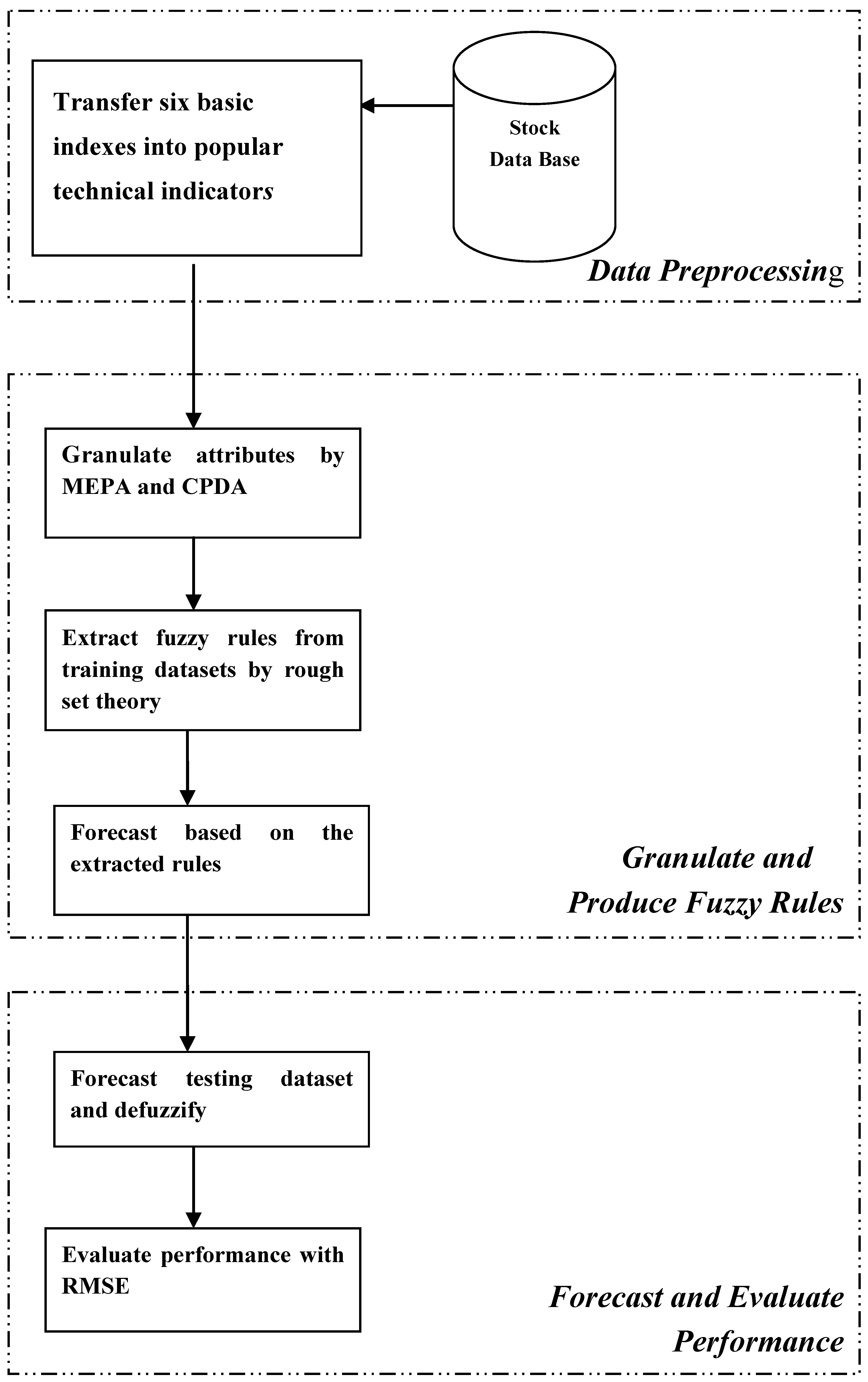
To overcome the problems mentioned above, a novel forecasting model (the framework of the proposed model is illustrated in Figure 3), which integrates two advanced data granulating approaches (CDPA and MEPA) and a data mining method (rough set theory) in forecasting processes, is proposed in this paper. The three main procedures of the proposed model are described, as follows:

(1) Data preprocess. Convert six basic indexes of the stock database (time, open index, high index, low index, close index, and volume) into nine useful technical indicators (RSI, MA, DIS, STOD, ROC, OBV, VR, PSY and AR, defined in Table 5), which are highly related to stock price fluctuation [2], in order to compose the attributes of experimental datasets.

(2) Granulate observations and produce rules. Utilize two advanced data granulating approaches, CPDA and MEPA, to granulate the observations of the nine technical indicators (defined in Table 5), and stock price fluctuation (defined in equation (17)) into linguistic values. The technical indicators are defined as conditional attributes and price fluctuation is defined as a decision attribute. Use a rough set algorithm (LEM2, Learning from Examples Module, version 2 [37]) to extract a training dataset to produce forecasting rules of linguistic values.

(3) Forecast and evaluate performance. Produce linguistic forecasts for testing a dataset with the extracted rules from a training dataset, and defuzzify the linguistic forecasts into numeric forecasts. Use root mean square error (RMSE) as a forecasting performance indicator for the proposed model. We argue that the proposed model can produce effective rules for forecasting stock market prices, based on three reasons, as follows:

Firstly, we employ technical indicators as forecasting factors instead of daily basic indexes; they are practical tools for stock analysts and fund managers to use in forecasting stock market prices Also, it has been proven that some technical indicators are highly related to future stock prices [2].

Secondly, from past literature related to rough set theory, three advantages have been found: (1) the rough set algorithms can process data without making any assumptions about the dataset; (2) rough set theory has powerful algorithms which can deal with a dataset that contains both quantitative and qualitative attributes; and (3) rough set algorithms can discover non-linear relations between observations hidden in multi-dimensional datasets, and produce understandable rules in an If-Then format that are meaningful to the average stock investor.

Lastly, the advantages to using data granulating methods to preprocess raw data are that the data dimension of a database can be reduced and simplified, and the use of discrete features is usually more compact and shorter than the use of continuous ones [38]. We argue that data granulating approaches can use linguistic values to represent observations in order to reduce the data complexity when using a high-dimension of a numeric dataset as an experimental dataset. Therefore, the proposed model can promote efficiency in data preprocess by employing CPDA and MEPA.

Figure 3. Framework of the proposed model.

Figure 3. Framework of the proposed model.

Table 5. Defined equations for popular technical indicators.

Technical Indicator	Mathematical Formula and Economical Meaning
MA	$\left[\frac{\text{sum of closing prices for a 6 - day period}}{6}\right]$
	●  MA is a popular way of defining where recent price trend line
RSI	$\left[\frac{\text{sum of positive closing prices for a 25 - day period}}{\text{sum of closing prices for a 25 - day period}}\times 100\right]$
	●  RSI, moving on a scale from 0–100, highlights overbought (70 and above) and oversold (30 and below) conditions
PSY	$\left[\frac{\text{number of days over a 12 - day period price closed up}}{12}\times 100\right]$
	●  PSY measures psychological stability of investors
STOD	$\left[\frac{\text{most recent closing price − 6 - day price low}}{\text{6 - day price high − 6 - day price low}}\times 100\right]$
	●  STOD gives buy (30 and below) or sell (70 and above) signals
VR	$\left[\frac{\begin{array}{l}\text{volume sum when price closed up for a 6 - day period −}\\ \text{volume sum when price closed down for a 6 - day period}\end{array}}{\text{the sum of volume over 6 days}}\times 100\right]$
	●  VR measures trend stability
OBV	$\left[\begin{array}{l}\text{volume sum when price closed up for a 6 - day period −}\\ \text{volume sum when price closed down for a 6 - day period}\end{array}\right]$
	●  OBV is a running cumulative total which should confirm the price trend
DIS	$\left[\frac{\text{most recent closing price}}{\text{6 - day MA}}\times 100\right]$
	●  DIS shows the stability of the most recent closing prices
AR	$\left[\frac{\text{high price − closing price}}{\text{opening price − low price}}\right]$
	●  AR shows stock momentum
ROC	$\left[\frac{\text{most recent closing price}}{\text{previous 6day price}}\right]$
	●  ROC gives buy (130 and above) and sell (70 and below) signals

Table 5. Defined equations for popular technical indicators.

Technical Indicator	Mathematical Formula and Economical Meaning
MA	$\left[\frac{\text{sum of closing prices for a 6 - day period}}{6}\right]$
	●  MA is a popular way of defining where recent price trend line
RSI	$\left[\frac{\text{sum of positive closing prices for a 25 - day period}}{\text{sum of closing prices for a 25 - day period}}\times 100\right]$
	●  RSI, moving on a scale from 0–100, highlights overbought (70 and above) and oversold (30 and below) conditions
PSY	$\left[\frac{\text{number of days over a 12 - day period price closed up}}{12}\times 100\right]$
	●  PSY measures psychological stability of investors
STOD	$\left[\frac{\text{most recent closing price − 6 - day price low}}{\text{6 - day price high − 6 - day price low}}\times 100\right]$
	●  STOD gives buy (30 and below) or sell (70 and above) signals
VR	$\left[\frac{\begin{array}{l}\text{volume sum when price closed up for a 6 - day period −}\\ \text{volume sum when price closed down for a 6 - day period}\end{array}}{\text{the sum of volume over 6 days}}\times 100\right]$
	●  VR measures trend stability
OBV	$\left[\begin{array}{l}\text{volume sum when price closed up for a 6 - day period −}\\ \text{volume sum when price closed down for a 6 - day period}\end{array}\right]$
	●  OBV is a running cumulative total which should confirm the price trend
DIS	$\left[\frac{\text{most recent closing price}}{\text{6 - day MA}}\times 100\right]$
	●  DIS shows the stability of the most recent closing prices
AR	$\left[\frac{\text{high price − closing price}}{\text{opening price − low price}}\right]$
	●  AR shows stock momentum
ROC	$\left[\frac{\text{most recent closing price}}{\text{previous 6day price}}\right]$
	●  ROC gives buy (130 and above) and sell (70 and below) signals

3.2. The Proposed Algorithm

The proposed algorithm consists of six forecasting processes. Using the 2001 TAIEX (Taiwan Stock Exchange Capitalization Weighted Stock Index) as demonstration data, each process is introduced, step by step, in the following manner:

Step 1: Transfer basic indexes into popular technical indicators. In this step, the stock database, which contains six basic indexes (time, open index, high index, low index, close index and volume) is selected as an experimental dataset. Each experimental dataset record (see Table 6) is transformed into a record of nine technical indicators (RSI, MA, DIS, STOD, ROC, OBV, VR, PSY and AR, see Table 7) by using the formulas in Table 5.

Table 6. Basic indexes of the TAIEX dataset.

Time	Open	High	Low	Close	Volume
2001/01/02	4,717.49	4,945.09	4,678.00	4,935.28	2,292,485
2001/01/03	4,843.54	4,970.45	4,831.12	4,20004.79	2,542,050
2001/01/04	5,028.32	5,169.13	5,028.32	5,136.13	3,146,064
2001/12/27	5,464.52	5,505.19	5,293.54	5,332.98	4,951,334
2001/12/28	5,372.85	5,408.15	5,307.38	5,398.28	4,035,088
2001/12/31	5,481.07	5,583.82	5,477.53	5,551.24	4,396,515

Table 6. Basic indexes of the TAIEX dataset.

Time	Open	High	Low	Close	Volume
2001/01/02	4,717.49	4,945.09	4,678.00	4,935.28	2,292,485
2001/01/03	4,843.54	4,970.45	4,831.12	4,20004.79	2,542,050
2001/01/04	5,028.32	5,169.13	5,028.32	5,136.13	3,146,064
2001/12/27	5,464.52	5,505.19	5,293.54	5,332.98	4,951,334
2001/12/28	5,372.85	5,408.15	5,307.38	5,398.28	4,035,088
2001/12/31	5,481.07	5,583.82	5,477.53	5,551.24	4,396,515

Table 7. Original data of conditional attributes and decision attribute.

Time	RSI	MA	DIS	STOD	ROC	OBV	VR	PSY	AR
2001/1/2	55.71	4737.20	100.03	−0.45	0.05	2335735.00	0.26	0.50	1.12
2001/1/3	55.89	4758.57	103.71	1.27	0.06	5941448.00	0.56	0.58	1.13
2001/1/4	60.40	4787.48	102.24	4.62	0.07	9906469.00	0.77	0.67	1.29
2001/12/27	49.82	5261.71	102.48	0.90	0.00	−2794502.00	−0.12	0.50	0.96
2001/12/28	51.92	5280.22	101.00	0.14	0.06	−2324048.00	−0.10	0.50	0.98
2001/12/31	52.29	5295.08	101.95	1.67	0.07	5669238.00	0.23	0.58	1.01

Table 7. Original data of conditional attributes and decision attribute.

Time	RSI	MA	DIS	STOD	ROC	OBV	VR	PSY	AR
2001/1/2	55.71	4737.20	100.03	−0.45	0.05	2335735.00	0.26	0.50	1.12
2001/1/3	55.89	4758.57	103.71	1.27	0.06	5941448.00	0.56	0.58	1.13
2001/1/4	60.40	4787.48	102.24	4.62	0.07	9906469.00	0.77	0.67	1.29
2001/12/27	49.82	5261.71	102.48	0.90	0.00	−2794502.00	−0.12	0.50	0.96
2001/12/28	51.92	5280.22	101.00	0.14	0.06	−2324048.00	−0.10	0.50	0.98
2001/12/31	52.29	5295.08	101.95	1.67	0.07	5669238.00	0.23	0.58	1.01

Step 2: Granulate conditional and decision attributes by MEPA and CPDA. In the experimental dataset, nine technical indicators are used as conditional attributes, and stock price fluctuations, defined in equation (17), is employed as a decision attribute:

price fluctuation(t) = P(t) − P(t − 1)

(17)

where price fluctuation (t) denotes the price change from time t − 1 to time t; P (t) denotes closing price at time t; and P(t − 1) denotes closing price at time t − 1.

This step granulates the numeric experimental dataset, which consists of two types of attributes (conditional and decision) into a granulated dataset of linguistic values for rule mining. The experimental dataset is preprocessed by two different approaches: CPDA is used to granulate the records of the decision attribute (stock price fluctuation), and MEPA is employed to granulate the records of the conditional attributes (nine technical indicators). The appropriate number of categories, based on human short-term memory function, is seven, and seven, plus or minus two [39]. Therefore, from the researchers’ perspective, the decision attribute is granulated with five linguistic values and the conditional attribute is granulated with seven linguistic values. The five linguistic values used to present stock price fluctuations are introduced, as follows: L1 denotes going up sharply; L2 denotes going up; L3 denotes remaining flat; L4 denotes going down; and L5 denotes down sharply. Because a technical indicator value cannot be defined in meaningful terms, the seven linguistic values to represent a technical indicator are defined as seven labeled numbers (L1 through L7). Table 8 demonstrates five parameterized triangle fuzzy numbers for five linguistic values of stock price fluctuations. Table 9 demonstrates the seven linguistic values (fuzzy numbers) and their corresponding numeric ranges for the conditional attribute of MA. Table 10 lists some observations for conditional and decision attributes for the experimental datasets.

Table 8. Parameterized fuzzy numbers for decision attributes (price fluctuation).

Linguistic Value	Fuzzy Number(a, b, c)
	a	b	c
L1	−560.2145	−323.297	−86.3797
L2	−126.9697	−79.5363	−32.1029
L3	−57.1115	−21.2323	14.647
L4	−8.728	30.0979	68.9238
L5	39.6556	349.08	658.5045
Standard Derivation = 92.26; Mean = −8.73

Table 8. Parameterized fuzzy numbers for decision attributes (price fluctuation).

Linguistic Value	Fuzzy Number(a, b, c)
	a	b	c
L1	−560.2145	−323.297	−86.3797
L2	−126.9697	−79.5363	−32.1029
L3	−57.1115	−21.2323	14.647
L4	−8.728	30.0979	68.9238
L5	39.6556	349.08	658.5045
Standard Derivation = 92.26; Mean = −8.73

Table 9. Parameterized fuzzy numbers for conditional attributes (MA).

Linguistic Value	Fuzzy Number(a,b,c)
	a	b	c
L1	8706.911	6617.774	4528.637
L2	4003.256	4597.310	5191.364
L3	4893.189	5297.220	5701.251
L4	5455.389	5816.147	6176.905
L5	5939.078	6312.935	6686.792
L6	6422.766	6886.143	7349.519
L7	6984.966	9151.448	11317.93
Standard Derivation =1321.17; Mean = 5939.08

Table 9. Parameterized fuzzy numbers for conditional attributes (MA).

Linguistic Value	Fuzzy Number(a,b,c)
	a	b	c
L1	8706.911	6617.774	4528.637
L2	4003.256	4597.310	5191.364
L3	4893.189	5297.220	5701.251
L4	5455.389	5816.147	6176.905
L5	5939.078	6312.935	6686.792
L6	6422.766	6886.143	7349.519
L7	6984.966	9151.448	11317.93
Standard Derivation =1321.17; Mean = 5939.08

Table 10. Observations for conditional and decision attributes (TAIEX).

Time	RSI	MA	DIS	STOD	ROC	OBV	VR	PSY	AR	Price Fluctuation
2001/01/02	L4	L1	L5	L7	L6	L7	L7	L5	L2	L1
2001/01/03	L4	L1	L6	L7	L7	L7	L7	L5	L3	L3
2001/01/04	L4	L1	L6	L7	L7	L7	L7	L5	L4	L5
2001/12/27	L3	L2	L6	L7	L5	L7	L3	L5	L1	L3
2001/12/28	L3	L2	L6	L7	L7	L7	L3	L5	L1	L3
2001/12/31	L3	L2	L6	L7	L7	L7	L7	L5	L1	L3

Table 10. Observations for conditional and decision attributes (TAIEX).

Time	RSI	MA	DIS	STOD	ROC	OBV	VR	PSY	AR	Price Fluctuation
2001/01/02	L4	L1	L5	L7	L6	L7	L7	L5	L2	L1
2001/01/03	L4	L1	L6	L7	L7	L7	L7	L5	L3	L3
2001/01/04	L4	L1	L6	L7	L7	L7	L7	L5	L4	L5
2001/12/27	L3	L2	L6	L7	L5	L7	L3	L5	L1	L3
2001/12/28	L3	L2	L6	L7	L7	L7	L3	L5	L1	L3
2001/12/31	L3	L2	L6	L7	L7	L7	L7	L5	L1	L3

Step 3: Extracted fuzzy rules from training datasets by Rough Set Theory. In this step, the experimental dataset of linguistic values is split into two datasets, training and testing. The training dataset is extracted by a rough set algorithm (LEM2, Learning from Examples Module, version 2 [37]) to produce rules for forecasting the future price. Table 11 lists some raw rules extracted from the training dataset. The rules can be expressed in the format of “If-Then” (Table 12 demonstrates three rules).

Table 11. Examples of rules extracted from training dataset using rough set algorithm.

Conditional Attribute										Decision Attribute
Rule 1	(OBV=L7)	(PSY=L5)	(MA=L1)	(STOD=L7)	(DIS=L6)	(ROC=L6)	(AR=L1)	(RSI=L2)	(VR=L4)	(decision=L3)
Rule 2	(OBV=L7)	(PSY=L5)	(MA=L1)	(DIS=L5)	(AR=L1)	(RSI=L1)	(STOD=L1)	N.A	N.A	(decision=L3)
Rule 3	(OBV=L7)	(PSY=L5)	(STOD=L7)	(MA=L1)	(RSI=L4)	(VR=L7)	(DIS=L6)	(ROC=L7)	(AR=L3)	(decision=L3)
Rule n-2	(OBV=L7)	(STOD=L7)	(PSY=L5)	(MA=L1)	(RSI=L4)	(VR=L7)	(DIS=L6)	(ROC=L6)	(AR=L6)	(decision=L4)
Rule n-1	(OBV=L7)	(AR=L1)	(MA=L1)	(PSY=L5)	(DIS=L5)	(ROC=L5)	(RSI=L2)	(STOD=L2)	(VR=L3)	(decision=L2)
Rule n	(OBV=L7)	(AR=L1)	(MA=L1)	(PSY=L5)	(DIS=L5)	(ROC=L5)	(RSI=L2)	(VR=L4)	(STOD=L2)	(decision=L2)

Table 11. Examples of rules extracted from training dataset using rough set algorithm.

Conditional Attribute										Decision Attribute
Rule 1	(OBV=L7)	(PSY=L5)	(MA=L1)	(STOD=L7)	(DIS=L6)	(ROC=L6)	(AR=L1)	(RSI=L2)	(VR=L4)	(decision=L3)
Rule 2	(OBV=L7)	(PSY=L5)	(MA=L1)	(DIS=L5)	(AR=L1)	(RSI=L1)	(STOD=L1)	N.A	N.A	(decision=L3)
Rule 3	(OBV=L7)	(PSY=L5)	(STOD=L7)	(MA=L1)	(RSI=L4)	(VR=L7)	(DIS=L6)	(ROC=L7)	(AR=L3)	(decision=L3)
Rule n-2	(OBV=L7)	(STOD=L7)	(PSY=L5)	(MA=L1)	(RSI=L4)	(VR=L7)	(DIS=L6)	(ROC=L6)	(AR=L6)	(decision=L4)
Rule n-1	(OBV=L7)	(AR=L1)	(MA=L1)	(PSY=L5)	(DIS=L5)	(ROC=L5)	(RSI=L2)	(STOD=L2)	(VR=L3)	(decision=L2)
Rule n	(OBV=L7)	(AR=L1)	(MA=L1)	(PSY=L5)	(DIS=L5)	(ROC=L5)	(RSI=L2)	(VR=L4)	(STOD=L2)	(decision=L2)

Step 4: Forecast based on the extracted rules. This step maps the conditional attributes of every record in the testing dataset with the extracted rules from the training dataset (see Table 11) in order to generate a linguistic forecast for future price trends. If the conditional attributes of a record satisfy the “If” criteria of a specific rule, the linguistic forecast for this instance is defined as the “Then” part of the rule. Whenever no rule can be found for the conditional attributes of a record, the naïve forecast [40] is employed as the forecast for the future price trend. Table 13 demonstrates the linguistic conditional attributes of some records and their corresponding linguistic forecasts for a testing dataset.

Table 12. IF-THEN rules.

Rules No.	If-Then Rules
Rule 1.	If (OBV=L7)& (PSY=L5) & (MA=L1) & (STOD=L7)& (DIS=L6) & (ROC=L6) & (AR=L1) & (RSI=L2)&(VR=L4) Then (Decision=L3)
Rule 2.	If (OBV=L7)& (PSY=L5) & (MA=L1) & (DIS=L5) & (AR=L1) & (RSI=L1)& (STOD=L1) Then (Decision=L3)
Rule 3.	If (OBV=L7)& (PSY=L5)&(STOD=L7)&(MA=L1)&(RSI=L4) &(VR=L7) & (DIS=L6) & (ROC=L7) & (AR=L3) Then (Decision=L3)

Table 12. IF-THEN rules.

Rules No.	If-Then Rules
Rule 1.	If (OBV=L7)& (PSY=L5) & (MA=L1) & (STOD=L7)& (DIS=L6) & (ROC=L6) & (AR=L1) & (RSI=L2)&(VR=L4) Then (Decision=L3)
Rule 2.	If (OBV=L7)& (PSY=L5) & (MA=L1) & (DIS=L5) & (AR=L1) & (RSI=L1)& (STOD=L1) Then (Decision=L3)
Rule 3.	If (OBV=L7)& (PSY=L5)&(STOD=L7)&(MA=L1)&(RSI=L4) &(VR=L7) & (DIS=L6) & (ROC=L7) & (AR=L3) Then (Decision=L3)

Table 13. Linguistic forecasts for testing dataset.

Time	RSI	MA	DIS	STOD	ROC	OBV	VR	PSY	AR	Linguistic Forecast
2001/11/01	L3	L1	L5	L7	L5	L7	L4	L5	L1	L3
2001/11/02	L4	L1	L5	L7	L5	L7	L2	L5	L3	L3
2001/11/05	L4	L1	L6	L7	L5	L7	L2	L5	L3	L3
2000/12/28	L3	L2	L6	L7	L7	L7	L3	L5	L3	L3
2000/12/31	L3	L2	L6	L7	L7	L7	L7	L5	L3	L3

Table 13. Linguistic forecasts for testing dataset.

Time	RSI	MA	DIS	STOD	ROC	OBV	VR	PSY	AR	Linguistic Forecast
2001/11/01	L3	L1	L5	L7	L5	L7	L4	L5	L1	L3
2001/11/02	L4	L1	L5	L7	L5	L7	L2	L5	L3	L3
2001/11/05	L4	L1	L6	L7	L5	L7	L2	L5	L3	L3
2000/12/28	L3	L2	L6	L7	L7	L7	L3	L5	L3	L3
2000/12/31	L3	L2	L6	L7	L7	L7	L7	L5	L3	L3

Step 5: Defuzzify and forecast testing datasets. Max membership principle [25] (see equation (16)) is employed to defuzzify the linguistic forecast from Step 4. After a linguistic forecast has been defuzzified to a numeric value, a numeric forecast (see Table 14) for a future stock price is generated by equation (18):

F(t) = P(t − 1) + f (t)

(18)

where P(t − 1) denotes the stock price at time t − 1; f (t) denotes the numeric value defuzzified from the linguistic forecast for the future price trend at time t; and F(t) denotes the numeric forecast for the future stock price at time t.

Step 6: Evaluate performance with RMSE. In this step, RMSE (defined in equation (19)) is used as a performance indicator for the proposed model. Table 15 demonstrates some forecasts produced from the proposed model and how to compute RMSE as a performance datum:

(19)

where P(t) denotes the actual stock price at time t; F(t) denotes the forecast at time t; and n is the total amount of forecasts.

Table 14. Numeric forecasting value for testing dataset.

Date	RSI	MA	DIS	STOD	ROC	OBV	VR	PSY	AR	Linguistic Forecast	Numeric Forecast
2001/11/01	L3	L1	L5	L7	L5	L7	L4	L5	L1	L3	3,882.49
2001/11/02	L4	L1	L5	L7	L5	L7	L2	L5	L3	L3	3,882.00
2001/11/05	L4	L1	L6	L7	L5	L7	L2	L5	L3	L3	3,908.69
2001/12/28	L3	L2	L6	L7	L7	L7	L3	L5	L1	L3	5,371.43
2001/12/31	L3	L2	L6	L7	L7	L7	L7	L5	L1	L3	5,311.98

Table 14. Numeric forecasting value for testing dataset.

Date	RSI	MA	DIS	STOD	ROC	OBV	VR	PSY	AR	Linguistic Forecast	Numeric Forecast
2001/11/01	L3	L1	L5	L7	L5	L7	L4	L5	L1	L3	3,882.49
2001/11/02	L4	L1	L5	L7	L5	L7	L2	L5	L3	L3	3,882.00
2001/11/05	L4	L1	L6	L7	L5	L7	L2	L5	L3	L3	3,908.69
2001/12/28	L3	L2	L6	L7	L7	L7	L3	L5	L1	L3	5,371.43
2001/12/31	L3	L2	L6	L7	L7	L7	L7	L5	L1	L3	5,311.98

Table 15. Forecasting value and performance with RMSE.

Time	Actual Stock Index	Forecast Value	SE(square error)
2001/11/01	3,929.69	3,882.00	2227.84
2001/11/02	3,998.48	3,908.69	8062.24
2001/11/05	4,080.51	3,977.48	10615.18
2001/12/28	5,398.28	5,311.98	7447.69
2001/12/31	5,551.24	5,377.28	30262.08
Mean of SE			14884
RMSE			122

Table 15. Forecasting value and performance with RMSE.

Time	Actual Stock Index	Forecast Value	SE(square error)
2001/11/01	3,929.69	3,882.00	2227.84
2001/11/02	3,998.48	3,908.69	8062.24
2001/11/05	4,080.51	3,977.48	10615.18
2001/12/28	5,398.28	5,311.98	7447.69
2001/12/31	5,551.24	5,377.28	30262.08
Mean of SE			14884
RMSE			122

4. Experiment and Comparisons

4.1. Experiment Dataset and Performance Indicator

In the evaluation experiments for the proposed model, a five-year period (2001–2005) of the TAIEX database was selected as the experimental dataset. Each year of the stock data is used as a unit of experimental dataset, where a ten-month period of stock data, from January to October, is used for training, and the rest, from November to December, for testing. To compare the performance of the proposed model with fuzzy time-series models, a common formula of forecasting error, root mean square error (RMSE) [6,19,41], is used as a performance indicator in this paper.

4.2. Model Verification

In order to evaluate the efficacy of the proposed model, vis-à-vis different types of time-series models, a two-part model comparison is provided: (1) performance comparisons with fuzzy time-series models, using one forecasting factor; and (2) performance comparisons with time-series models, using multiple forecasting factors. In the first part, the purpose is to examine whether there is more information hidden in the selected technical indicators (RSI, MA, DIS, STOD, ROC, OBV, VR, PSY and AR) than basic indexes (time and close index). Therefore, two past fuzzy time-series models, based on stock price time-series, Chen’s (1996) [11], Huarng et al.’s (2006) [6], are employed as comparison models. In the second part, the purpose is to verify the superiority of the proposed model. Therefore, two forecasting models using multiple forecasting factors, Cheng et al.’s model [41] and a multiple regression model (MLR) [42], are employed for purposes of comparison.

Figure 4. Performance comparisons with single-factor forecasting models.

Figure 4. Performance comparisons with single-factor forecasting models.

Table 16. Performance comparisons with single-factor forecasting models.

	Year	2001	2002	2003	2004	2005	Average	Variance
Models
Chen’s Model (1996) [11]		148	101	74	83	66	94	854
Huarng et al.’s Model (2006) [6]		130	*84	56	79	69	84	630
Proposed Model		*122	94	*55	*69	*65	*81	*580

* denotes the minimum value among three models.

Table 16. Performance comparisons with single-factor forecasting models.

	Year	2001	2002	2003	2004	2005	Average	Variance
Models
Chen’s Model (1996) [11]		148	101	74	83	66	94	854
Huarng et al.’s Model (2006) [6]		130	*84	56	79	69	84	630
Proposed Model		*122	94	*55	*69	*65	*81	*580

* denotes the minimum value among three models.

From the experimental results for the first part of the performance comparisons, listed in Table 16 and illustrated in Figure 4, it is clear that the proposed model outperforms Chen’s (1996) [11] and Huarng et al.’s (2006) [6] models. Among the three models, the proposed model bears the smallest RMSE for four of the five experimental datasets (2001, 2003, 2004 and 2005). The proposed model also holds the smallest value of average RMSE (81) among the comparison models (94 for Chen’s model [11] and 84 for Huarng et al.’s model [6]). Further, the variance of RMSE for the proposed model is the smallest (580 for the proposed model, 854 for Chen’s model and 630 for Huarng et al.’s model [6]). The smallest variance implies that the proposed model performs with more stability than the other two models.

Figure 5. Performance comparisons with multiple-factor forecasting models.

Figure 5. Performance comparisons with multiple-factor forecasting models.

Table 17. Performance comparisons with multiple-factor forecasting models.

	Year	2001	2002	2003	2004	2005	Average	Variance
Models
Multiple Regression Model [42]		630	*66	804	820	144	493	105310
Cheng et al.’s Model (2008) [41]		531	606	800	146	229	462	58777
Proposed Model		*122	94	*55	*69	*65	*81	*585

* denotes minimum value among three models.

Table 17. Performance comparisons with multiple-factor forecasting models.

	Year	2001	2002	2003	2004	2005	Average	Variance
Models
Multiple Regression Model [42]		630	*66	804	820	144	493	105310
Cheng et al.’s Model (2008) [41]		531	606	800	146	229	462	58777
Proposed Model		*122	94	*55	*69	*65	*81	*585

* denotes minimum value among three models.

From the experimental results for the first part of the performance comparisons, listed in Table 17 and illustrated in Figure 5, we may note that the proposed model still performs with the smallest RMSE in four testing datasets (2001, 2003, 2004 and 2005) and the smallest average RMSE (81 for the proposed model, 493 for multiple regression model, and 462 for Cheng et al’s model [41]). Additionally, in the stability analysis, the proposed model has better forecasting stability than the other two multiple-factor forecasting models, based on the variance of RMSE (585 for the proposed model, 105310 for Multiple Regression Model [42], and 58777 for Cheng et al’s model [41]).

As the performance datum above adduces, the proposed model demonstrates outstanding performance and stability in forecasting Taiwan’s stock market trends.

5. Conclusions and Future Research

In this paper, one novel forecasting model, based on two advanced granulating methods (MEPA and CDPA), and rough set theory, is proposed to provide understandable rules for the average stock investor and to improve forecasting accuracy of Taiwan’s stock market. Based on the model verification, we argue that the proposed model has reached the research objectives. After implementing the experiment for evaluating the proposed model, three findings are noted, as follows:

Firstly, technical indicators can provide more information for forecasting future stock prices. In practical stock market analysis, multiple-technical indicators can posit more meaningful stock information, such as stock price trends, fluctuations and momentums, and many stock analysts do employ technical indicators to analyze market trends. However, past fuzzy time-series models such as Chen’s (1996) [11], and Huarng et al.’s (2006) [6] employed only one forecasting factor, past stock price, to predict the future stock price. The single forecasting factor is absolutely insufficient to reveal the complex relationships within a stock market. Regarding the forecasting model using basic indexes (time, open index, high index, low index, close index and volume) as multiple forecasting factors, such as Cheng et al.’s model [41] and multiple regression model (MLR) [42], we argue that the basic indexes cannot provide useful stock information for forecasting stock markets because they can only display static statistics of stock markets not dynamic market trends and fluctuations. From performance comparisons (see Table 16 and Table 17), it is clear that the proposed model outperforms the four listed models, Chen’s (1996) [11], Huarng et al.’s (2006) [6] models, Cheng et al.’s [41] and MLR [42]. The evidence has proven this finding.

Secondly, granulating methods can reduce the complexity of experiments using high-dimension datasets. The proposed model employs MEPA and CPDA to produce linguistic values for conditional and decision attributes, which can make the rule-extracting process of rough set algorithm simpler and faster.

Lastly, rough set algorithm can find useful rules from historical stock data for investment decision-making. From Table 11 and Table 12, the rules extracted by rough set algorithm can be used as investment decision suggestions for average investors. Although a linguistic forecast, generated by the rules, cannot be employed as a forecasting value, the proposed model has provided a valid defuzzifying method to produce an accurate forecasting value, based on the linguistic forecast, to predict future stock prices.

For future research, two suggestions are offered: (1) other financial markets, such as commodity futures and mutual funds can be used as forecasting targets to evaluate the proposed model; and (2) other modifying models, such as adaptive expectation models and neural networks can be used to modify the forecasts, produced from the proposed model, enabling more accurate forecasts.

References

1. Marshall, B.R.; Cahan, R.H.; Caha, J.R. Does intraday technical analysis in the U.S. equity market have value? J. Empirical Finance 2008, 15, 199–210. [Google Scholar] [CrossRef]
2. Kim, M.J.; Min, S.H.; Han, I. An evolutionary approach to the combination of multiple classifiers to predict a stock price index. Expert Syst. Appl. 2006, 32, 241–247. [Google Scholar] [CrossRef]
3. Yamawaki, M.T.; Tokuoka, S. Adaptive use of technical indicators for the prediction of intra-day stock prices. Physica A 2007, 383, 125–133. [Google Scholar] [CrossRef]
4. Thomas, R.D. The New Science of Technical Analysis; Wiley: New York, NY, USA, 1994. [Google Scholar]
5. Bauer, R.J., Jr. Genetic Algorithms and Investment Strategies; Wiley: New York, NY, USA, 1994. [Google Scholar]
6. Huarng, K.H.; Yu, T.H.K. The application of neural networks to forecast fuzzy time series. Physica A 2006, 336, 481–491. [Google Scholar] [CrossRef]
7. Refenes, A.N.; Burgess, N.; Bentz, Y. Neural networks in financial engineering: A study in methodology. IEEE Trans. Neural Networks 1997, 8, 1222–1267. [Google Scholar] [CrossRef] [PubMed]
8. Trippi, R.R.; Turban, E. Neural Network in Finance and Investing; Turban, E., Ed.; Probus Publishing Company: Chicago, IL, USA, 1993. [Google Scholar]
9. Azo, M.E. Neural Network Time Series Forecasting of Financial Markets; Wiley: New York, NY, USA, 1994. [Google Scholar]
10. Gately, E. Neural Networks for Financial Forecasting; Wiley: New York, NY, USA, 1996. [Google Scholar]
11. Chen, S.M. Forecasting enrollments based on fuzzy time-series. Fuzzy Set. System. 1996, 81, 311–319. [Google Scholar] [CrossRef]
12. Mani, G.; Quah, K.K.; Mahfoud, S.; Barr, D. An analysis of neural-network forecasts from a large-scale, real-world stock selection system. In Proceedings of the IEEE/IAFE Conference on Computational Intelligence for Financial Engineering, New York, NY, USA, April 1995; pp. 72–78.
13. Skalko, C. Rough sets help time the OEX. J. Comput. Intell. Finance 1996, 4, 20–27. [Google Scholar]
14. Christensen, R. Entropy Minimax Sourcebook; Entropy Ltd.: Loncoln, MA, USA, 1980. [Google Scholar]
15. Yager, R.; Filev, D. Template-based fuzzy system modeling. J. Intell. Fuzzy Syst. 1994, 2, 39–54. [Google Scholar]
16. Chen, J.R.; Cheng, C.H. Extracting classification rules of software diagnosis using modified MEPA. Expert Syst. Appl. 2008, 34, 411–418. [Google Scholar] [CrossRef]
17. Cheng, C.H.; Chen, T.L.; Wei, L.Y. A hybrid model based on rough sets theory and genetic algorithms for stock price forecasting. Inform. Sci. 2010, 180, 1610–1629. [Google Scholar] [CrossRef]
18. Chen, J.R.; Chou, H.L.; Tai, D.W.S. Feature selection based on modified minimize entropy principle. In Proceedings of The International Conference On lectronics and Information Engineering, Kyoto, Japan, August 2010; pp. 10–13.
19. Teoh, H.J.; Cheng, C.H.; Chu, H.H.; Chen, J.S. Fuzzy time series model based on probabilistic approach and rough set rule induction for empirical research in stock markets. Data Knowl. Eng. 2008, 67, 103–117. [Google Scholar] [CrossRef]
20. Hardianto, I.; Maury, A.N. An evaluation of cumulative probability distribution of force (CPDF) as an exposure assessment method during isometric non-isotonic shoulder abductions. Int. J. Ind. Ergonomic. 2006, 36, 37–43. [Google Scholar]
21. Pawlak, Z. Rough sets. Int. J. Comput. Inform. Sci. 1982, 11, 341–356. [Google Scholar] [CrossRef]
22. Pal, S.K.; Skowron, A. Rough Fuzzy Hybridization: A New Trend in Decision Making; Springer: Singapore, 1999. [Google Scholar]
23. Pai, P.F.; Chen, S.Y.; Huang, C.W.; Chang, Y.H. Analyzing foreign exchange rates by rough set theory and directed acyclic graph support vector machines. Expert Syst. Appl. 2010, 37, 5993–5998. [Google Scholar] [CrossRef]
24. Pai, P.F.; Lee, F.C. A rough set based model in water quality analysis. Water Resour. Manag. 2010, 24, 2405–2418. [Google Scholar] [CrossRef]
25. Ross, T.J. Fuzzy Logic with Engineering Applications, International ed.; McGraw-Hill: New York, NY, USA, 2000. [Google Scholar]
26. Yeh, C.A. New Fuzzy Time Series Approaches for Forecasting in Expenditure of Information Project. Dissertation of Master Degree, Institute of Information Management, National Yunlin University of Science and Technology, Yunlin, Taiwan, June 2004. [Google Scholar]
27. Dallal, G.E.; Wilkinson, L. An analytic approximation to the distribution of Lilliefors' test for normality. Amer. Statist. 1986, 40, 294–296. [Google Scholar]
28. Teoh, H.J.; Cheng, C.H.; Chu, H.H.; Chen, J.S. Fuzzy time series model based on probabilistic approach and rough set rule induction for empirical research in stock markets. Data Knowl. Eng. 2008, 67, 103–117. [Google Scholar] [CrossRef]
29. Math Works Incorporation. Internet Communication. 30 October 2010. Available online: http://www.mathworks.com/help/toolbox/stats/normcdf.html (accessed on 30 October 2010).
30. Acklam, P.J. Internet Communication. 30 May 2008. Available online: http://home.online.no/~pjacklam/notes/invnorm/ (accessed on 30 May 2008).
31. Zadeh, L. A. Fuzzy sets. Inform. Contr. 1965, 8, 338–353. [Google Scholar] [CrossRef]
32. Pawlak, Z.; Skoworn, A. Rudiments of rough sets. Inform. Sci. 2007, 177, 3–27. [Google Scholar] [CrossRef]
33. Xu, B.; Zhou, Y.; Lu, H. An improved accuracy measure for rough sets. J. Comput. Syst. Sci. 2005, 71, 163–173. [Google Scholar] [CrossRef]
34. Wong, J.T.; Chung, Y.S. Rough set approach for accident chains exploration. Accid. Anal. Prevent. 2007, 39, 629–637. [Google Scholar] [CrossRef] [PubMed]
35. Chen, S.M.; Chung, N.Y. Forecasting enrollments using high-order fuzzy time series and genetic algorithms. Int. J. Intell. Syst. 2006, 21, 485–501. [Google Scholar] [CrossRef]
36. Arciszewski, T.; Ziarko, W. Inductive learning in civil engineering: A rough sets approach. Microcomput. Civil Eng. 1990, 5, 19–28. [Google Scholar] [CrossRef]
37. Grzymala-Busse, J.W. A New version of the rule induction system, LERS. Fundam. Inform. 1997, 31, 27–39. [Google Scholar]
38. Liu, H.; Hussain, F.; Tan, C.; ash, M. Discretization: An enabling technique. Data Min. Knowl. Discov. 2002, 6, 393–423. [Google Scholar] [CrossRef]
39. Miller, G.A. The magical number seven, plus or minus two: some limits on our capacity of processing information. Psychol. Rev. 1956, 63, 81–97. [Google Scholar] [CrossRef] [PubMed]
40. Atkeson, A.; Lee, E.O. Are Phillips curves useful for forecasting inflation? Fed. Res. Bank MN Q. Rev. 2001, 25, 2–11. [Google Scholar]
41. Cheng, C.H.; Cheng, G.W.; Wang, J.W. Multi-attribute fuzzy time series method based on fuzzy clustering. Expert Syst. Appl. 2008, 34, 1235–1242. [Google Scholar] [CrossRef]
42. Kendall, M.G. The analysis of economic time series, Part 1: Price. J. Roy. Statist. Soc. 1953, 96, 11–25. [Google Scholar] [CrossRef]