Representing Entropy with Dispersion Sets

Abstract

A novel representation of entropy is introduced, based on the heuristic concept of heat dispersion. To this end dispersion sets are defined, which describe both the heat transferred to a system and the associated entropy change. Some applications are discussed.

1. Introduction

Given that there are presently three “traditional understandings of entropy [which] include the thermodynamic approach of Clausius, the statistical mechanics approaches of Boltzmann and Gibbs and the information theory approach of Shannon” [1], it is still difficult to grasp the concept of entropy in an intuitive and straightforward way. It will be shown that connecting Clausius’ understanding of entropy with information about mean values in the microscopic world coming out from the statistical approach, an uncomplicated representation of entropy arises, which readily lends itself to be pictorially visualized.

2. Dispersion Sets

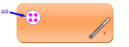
When a quantity of heat ΔQ is transferred to a system, the system undergoes a variation of entropy. This entropy variation will now be studied in more detail. Assuming that the heat ΔQ is small and that the speed at which it is transferred to the system is slow, in order to avoid significant perturbations of the system, Clausius defined the entropy variation of a material system to be:

$$\Delta S=\frac{\Delta Q}{T}$$

(1)

where T is the absolute temperature of the system. To represent the transferred heat ΔQ, a “dispersion set” is introduced here, defining it as an energetically equivalent collection of a certain number ΔN of degrees of freedom, each of which is bearing—in virtue of equipartition—the mean energy ½kT, where k is Boltzmann’s constant. The transferred heat can therefore be expressed as:

$$\Delta Q=\frac{1}{2}kT\cdot \Delta N$$

(2)

Substituting this expression into equation (1) the entropy variation reduces to:

$$\Delta S=\frac{1}{2}k\cdot \Delta N$$

(3)

According to the above equation, the entropy change ΔS varies in direct proportion with the cardinality ΔN of the corresponding dispersion set. This will now be discussed in depth.

3. Representing Entropy

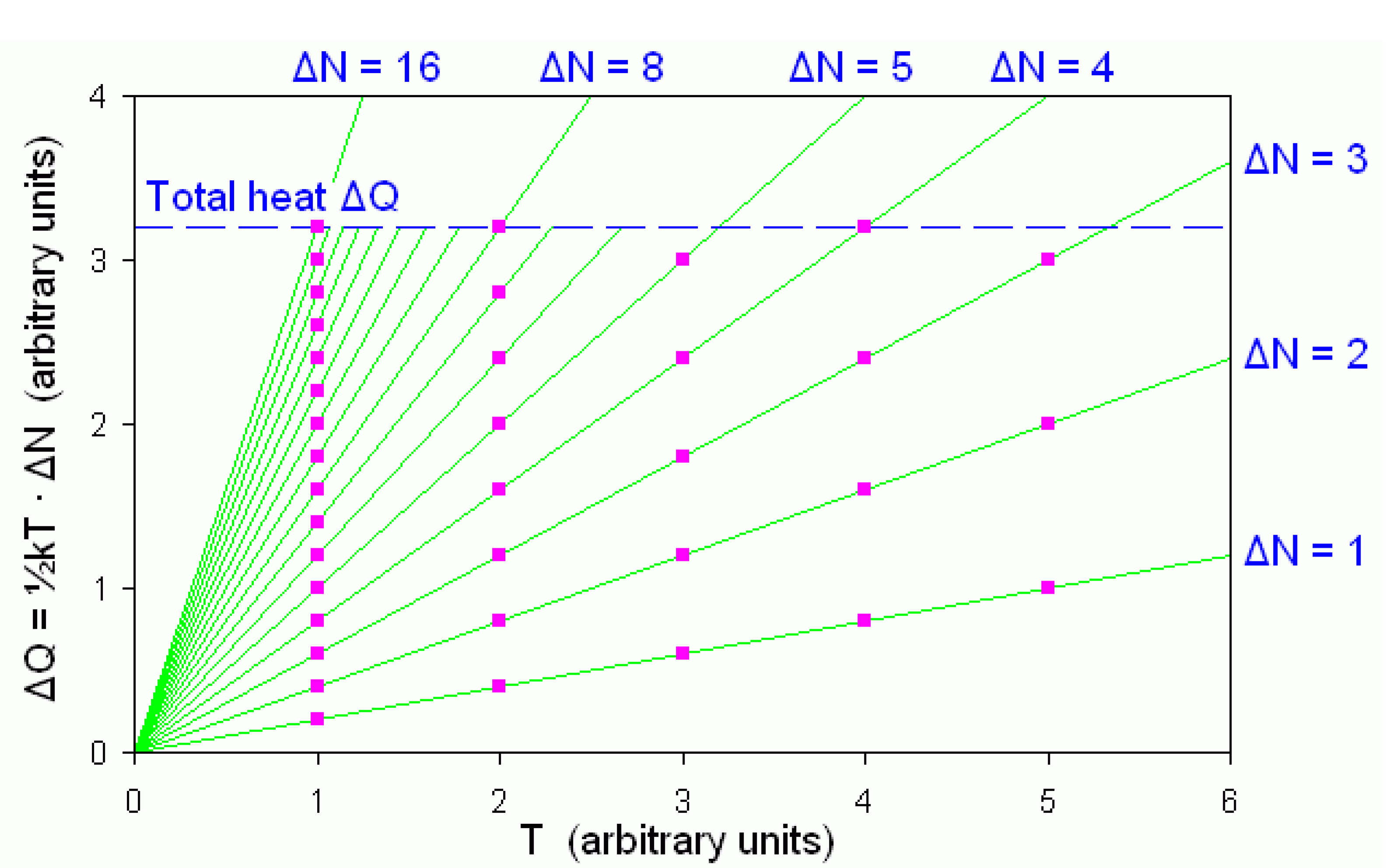
According to the above, any heat ΔQ that is transferred to a system is energetically equivalent to a dispersion set of ΔN degrees of freedom, whose mean energies ½kT are proportional to temperature. These degrees of freedom may be called “dispersion elements”, as they are constituents of a dispersion set. For a given ΔQ, the set’s cardinality ΔN varies inversely with temperature, as shown in Figure 1.

Figure 1. The dispersion elements making up a given heat ΔQ are marked as dots in vertical arrays below the dashed line. Each vertical array represents a dispersion set at the corresponding temperature. The cardinality of those sets varies inversely with temperature, as shown by the numbers ΔN appearing on the upper and right border of the figure.

Figure 1. The dispersion elements making up a given heat ΔQ are marked as dots in vertical arrays below the dashed line. Each vertical array represents a dispersion set at the corresponding temperature. The cardinality of those sets varies inversely with temperature, as shown by the numbers ΔN appearing on the upper and right border of the figure.

In reality the “dispersion cardinalities”, as the cardinalities ΔN of dispersion sets may concisely be called, are much greater than the cardinalities appearing in Figure 1. In fact, since in equation (2) Boltzmann’s constant k has—according to CODATA—the small value 1.3806504(24) · 10^–23 JK^–1, a heat ΔQ = 1 Joule will distribute e.g., with a dispersion cardinality ΔN = 4.83 · 10²⁰ at the earth’s average surface temperature of 300 K and with a dispersion cardinality ΔN = 2.41 · 10¹⁹ on the sun’s photosphere, whose temperature 6,000 K is 20 times higher.

Dividing these cardinalities by Avogadro’s constant N_A, they turn out to be equivalent to nearly 800 µmol and 40 µmol respectively. This molar form is particularly convenient when entropy is represented with dispersion sets. Equations (2) and (3) could themselves be given molar form substituting k ← R and ΔN ← Δn, where R is the molar gas constant and Δn the molar dispersion cardinality. However to keep things simple we don’t proceed along this route.

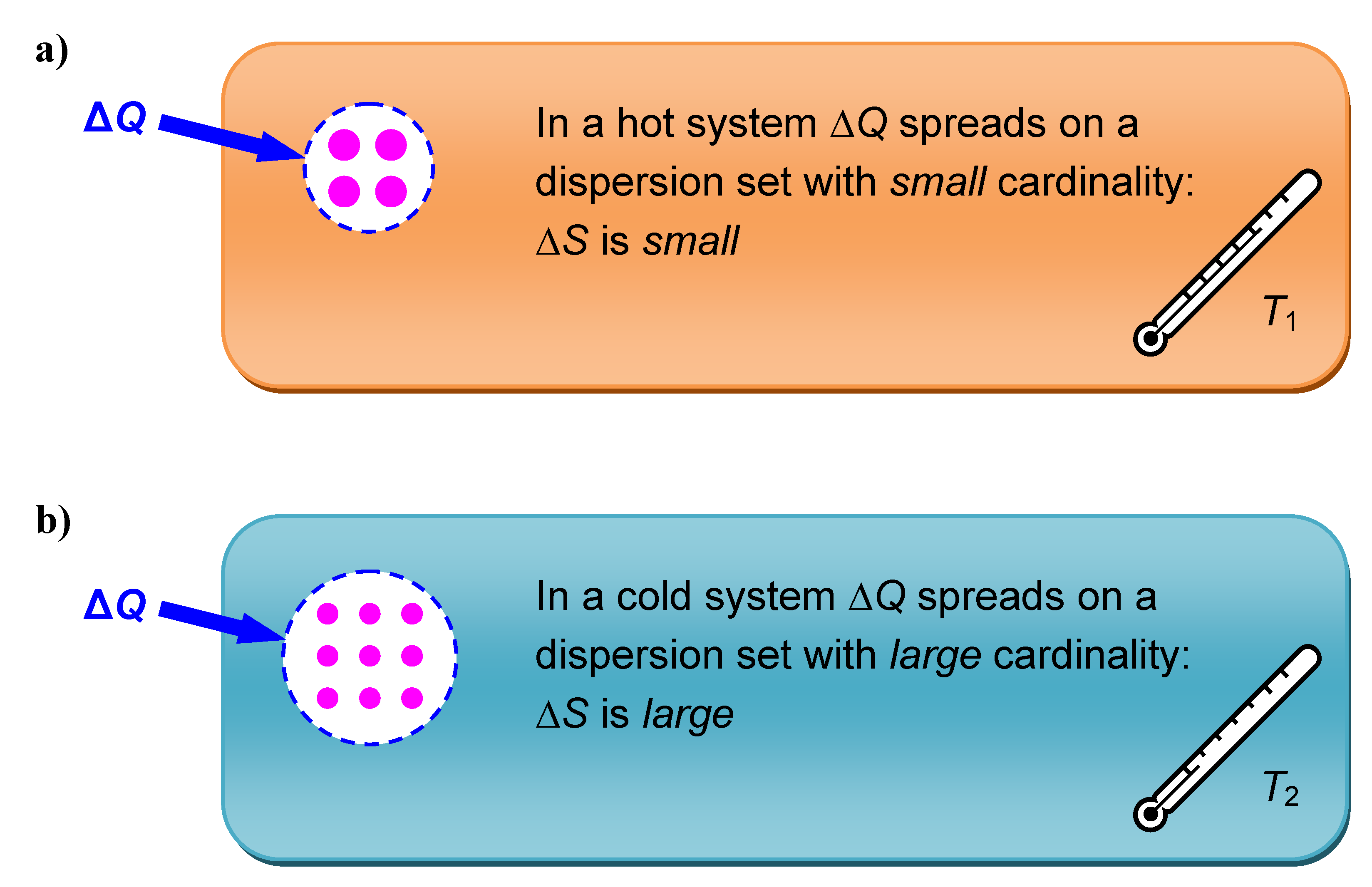
To sum up, it can be said that when a heat ΔQ is transferred to a system, it disperses onto a certain collection of “dispersion elements” and that the “dispersion cardinality” ΔN of the corresponding “dispersion set” is an expression of the entropy change occurring within the system. An illustration of this is given in Figure 2.

Figure 2. According to the temperature of the system—higher in a), lower in b)—a heat ΔQ that is transferred to a system disperses on more or less dispersion elements. The latter are sketched as small dots whose sizes conform to ½kT. Entropy changes according to the cardinality of the corresponding dispersion set, which is drawn within a dashed line.

Figure 2. According to the temperature of the system—higher in a), lower in b)—a heat ΔQ that is transferred to a system disperses on more or less dispersion elements. The latter are sketched as small dots whose sizes conform to ½kT. Entropy changes according to the cardinality of the corresponding dispersion set, which is drawn within a dashed line.

4. The Second Principle

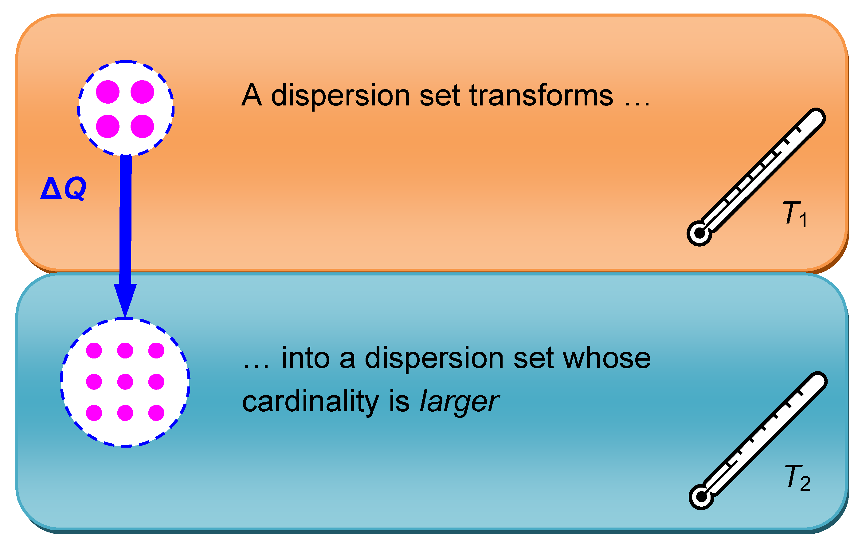
The second principle postulates that entropy cannot decrease in isolated systems. Any entropy increase that may possibly occur is then irreversible. This means that the heat contained in an isolated system always distributes in a way that does not decrease the cardinality of the associated dispersion set. Any—irreversible—increase of dispersion cardinality is explicitly allowed by the second principle. So for example the transfer of heat from a warmer to a colder subsystem, as illustrated in Figure 3, can easily take place.

To play with numbers, when the heat ΔQ = 1 Joule is transferred from the solar photosphere to the earth’s surface, from 6,000 K to 300 K, this deprives the sun of the equivalent of ΔN₁ = 40 µmol dispersion elements while the earth receives the equivalent of ΔN₂ = 800 µmol dispersion elements. In this transfer the heat ΔQ = 1 Joule clearly “improves” its dispersal. The net cardinality increment ΔN₂ – ΔN₁ = 760 µmol is a measure of the total entropy increase associated with the heat transfer.

Figure 3. When a heat ΔQ transfers from a subsystem with higher temperature to a subsystem with lower temperature with which it is in thermal contact, it distributes on a greater number of dispersion elements. While the first subsystem undergoes an entropy decrease, the second subsystem experiences an overcompensating entropy increase. Therefore the entropy of the whole system increases irreversibly.

Figure 3. When a heat ΔQ transfers from a subsystem with higher temperature to a subsystem with lower temperature with which it is in thermal contact, it distributes on a greater number of dispersion elements. While the first subsystem undergoes an entropy decrease, the second subsystem experiences an overcompensating entropy increase. Therefore the entropy of the whole system increases irreversibly.

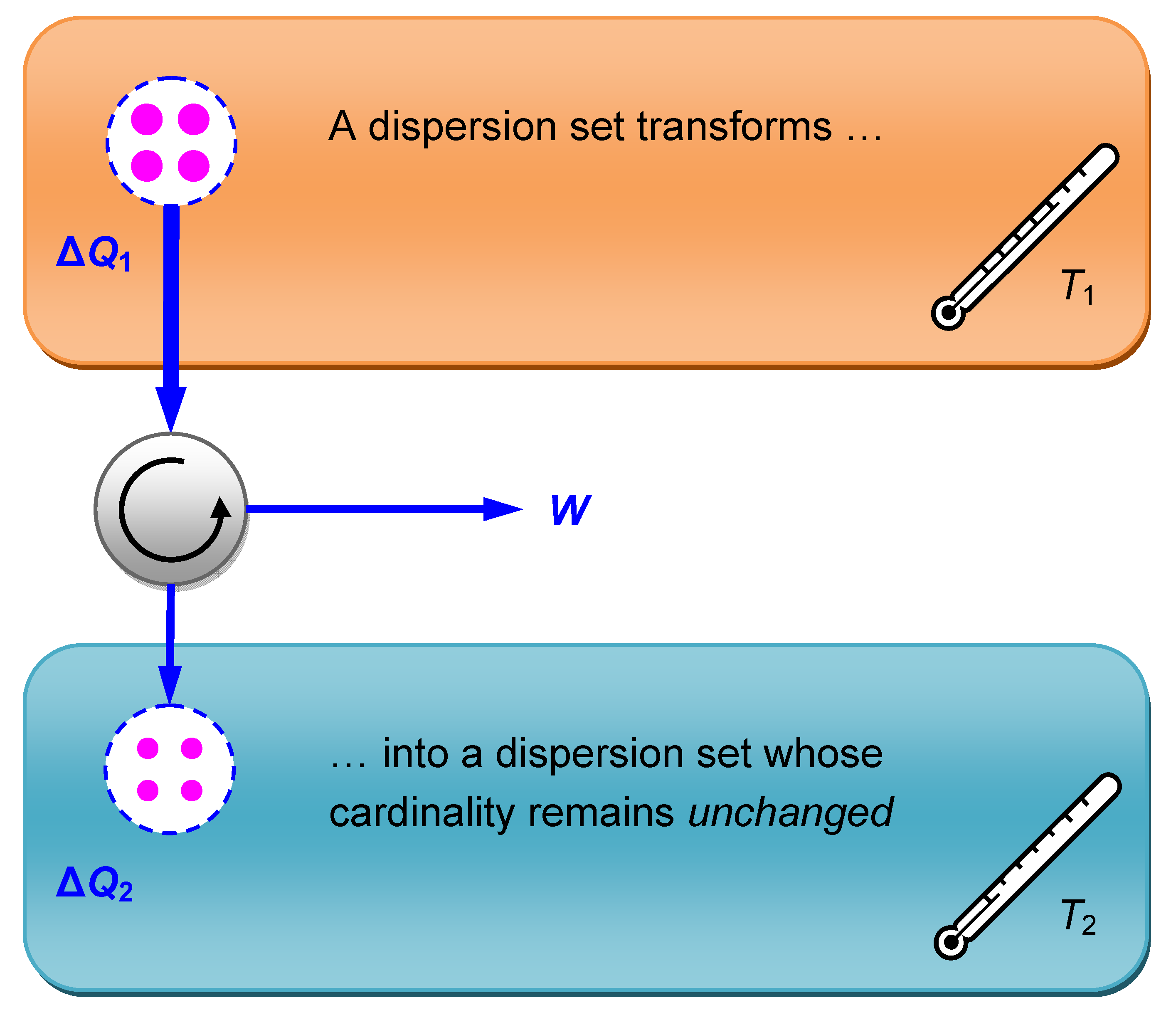
In Figure 3 the dispersion cardinality increases in virtue of the lower temperature of the receiving subsystem. But the heat transfer to the subsystem with lower temperature would also conform to the second principle if the dispersion cardinality wouldn’t increase that much. This could be accomplished with the aid of a device that branches off some energy W from the heat flow. Such a device is called a heat engine. Trying to improve the heat engine by branching off more and more energy W to do what in practical terms is called “useful work”, the dispersion cardinality will increase lesser and lesser. A limiting case is reached when the cardinality remains unchanged. According to the second principle no further improvement of the heat engine is possible beyond that point. This special case is shown in Figure 4.

Figure 4. When a heat ΔQ₁ runs through a heat engine—the circle between the two thermal subsystems—that branches off some energy from the heat flow, converting it into “useful work” W, the heat output ΔQ₂ must distribute on at least the same number of dispersion elements as the heat input. If, as in the limiting case shown below, the dispersion cardinality is unchanged, the entropy of the whole system remains constant.

Figure 4. When a heat ΔQ₁ runs through a heat engine—the circle between the two thermal subsystems—that branches off some energy from the heat flow, converting it into “useful work” W, the heat output ΔQ₂ must distribute on at least the same number of dispersion elements as the heat input. If, as in the limiting case shown below, the dispersion cardinality is unchanged, the entropy of the whole system remains constant.

5. Efficiency

In the situation illustrated in Figure 4 the heat engine achieves its maximum efficiency:

$${\eta }_{\max }=\frac{W}{\Delta Q_1}$$

(4)

This can be transformed as follows:

$${\eta }_{\max }=\frac{\Delta Q_1-\Delta Q_2}{\Delta Q_1}$$

(5)

$${\eta }_{\max }=\frac{\frac{1}{2}k{T}_1\cdot \Delta N-\frac{1}{2}k{T}_2\cdot \Delta N}{\frac{1}{2}k{T}_1\cdot \Delta N}$$

(6)

Reducing the quotient on the right side of equation (6) leads to the known result:

$${\eta }_{\max }=\frac{T_1-T_2}{T_1}$$

(7)

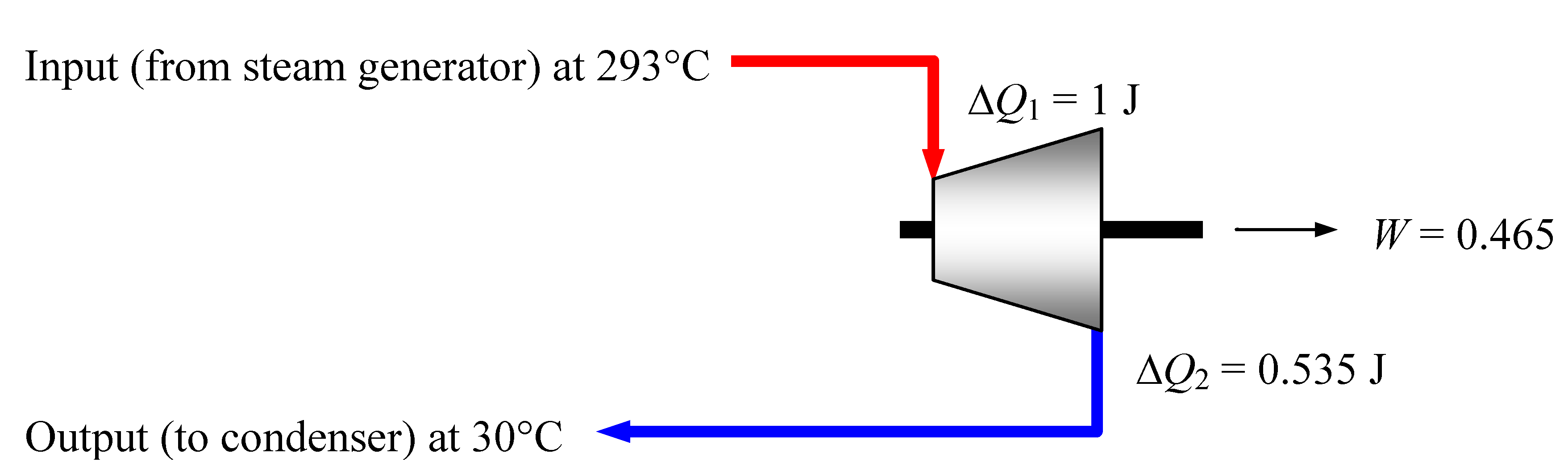
As an application let’s consider the 1,600 MWe EPR nuclear power plant that is actually under construction in Finland. According to the manufacturer’s specifications, its turbines are designed to work between the steam temperatures T₁ = 293°C and T₂ = 30°C [2]. If these favourable specifications—made possible by sea water cooling—can be maintained, equation (7) predicts a maximum thermal efficiency η_max of 46.5%. At this high efficiency a heat ΔQ₁ = 1 Joule, delivered to the turbines with a dispersion cardinality ΔN₁ = 425 µmol, would transform into an amount W = 0.465 Joule of useful work available at the turbine shaft and into a residual waste heat ΔQ₂ = 0.535 Joule dispersed with the same cardinality ΔN₂ = 425 µmol. Figure 5 represents the situation.

Figure 5. Finland’s EPR steam turbine system, hypothetically working at its maximum efficiency η max = 46.5%. An input heat of 1 Joule distributes so that ΔN₁ = ΔN₂ = 420 µmol. Maximum efficiency cannot however be achieved in practice (see Figure 7).

Figure 5. Finland’s EPR steam turbine system, hypothetically working at its maximum efficiency η max = 46.5%. An input heat of 1 Joule distributes so that ΔN₁ = ΔN₂ = 420 µmol. Maximum efficiency cannot however be achieved in practice (see Figure 7).

It should be noted that the equality of the cardinalities ΔN₁ and ΔN₂ can be maintained only at maximal efficiency. In reality however the thermal efficiency must necessarily be lower than η_max, as will be discussed in Section 8. So ΔN₂ must exceed ΔN₁, reducing the useful energy output W available at the turbine shaft. A calculation under more realistic conditions will be done at the end of Section 8.

Returning to Figure 4, it can be seen that reversing the heat and energy flows, this would represent the action a heat pump or of a refrigerator. Their coefficients of performance could be obtained with the same ease as the above maximum efficiency, repeating the steps from equation (4) to equation (7).

6. Radiation Systems

Radiation-specific quantum effects induce a departure from plain equipartition, so that, according to Planck’s radiation law, the oscillators in the cavity of a black body have a mean energy that decreases with increasing frequency. How can dispersion sets be defined under these circumstances for a black-body radiation system? As a definite energy is distributed on a finite number of quanta in the cavity, it is possible to determine a mean quantum energy, which, as is known, amounts to 2.7kT [3]. Therefore, when an amount of heat ΔQ is transferred to a system of black-body photons, it will distribute on some number ΔN of dispersion elements i.e. quanta with the mean energy 2.7kT.

To find a relation between entropy and dispersion elements, the steps leading form equation (1) to equation (3) will be repeated here, starting with Clausius’ definition:

$$\Delta S=\frac{\Delta Q}{T}$$

(8)

Writing the transferred heat in the form:

$$\Delta Q=2.7kT\cdot \Delta N$$

(9)

the entropy variation (8) reduces to:

$$\Delta S=2.7k\cdot \Delta N$$

(10)

Once again the entropy change is associated with the cardinality ΔN of a dispersion set, which now obviously consists of radiation quanta instead of mechanical degrees of freedom. Hence it is possible to adapt Figure 1 to Figure 4 to describe black-body radiation systems as well.

Figure 4, for example, could be related to the thermal radiation exchange occurring at the Earth’s surface. In fact the second principle imposes that in a given interval of time the earth emits at least the same number of infrared photons as visible photons coming from the sun are absorbed. The energy difference W is available for nonthermal transformations, e.g., to drive weather phenomena or biologic processes like photosynthesis.

According to what has been said above, the “entropic value” of solar radiation must not be seen in its supposed ability to deliver “negative entropy” [4] into our terrestrial environment but instead in the relatively big chunks of energy that its photons—emitted at 6,000 K—are made of. Because of their size, these 6,000 K-photons can transform and disperse in various forms to lower-energetic lumps in our 300 K-environment. The multiplicity of the possible downsizing phenomena allows a great variety of solar-driven processes—life included—to take place on the Earth’s surface.

When cardinalities are calculated for radiation systems according to equations (9) and (10), the resulting “photonic” cardinalities differ in value from the “mechanical” ones resulting from equations (2) and (3). This is due to the different numerical coefficients present in those equations. For example an energy ΔQ = 1 Joule in the black-body radiation emanating from the solar 6,000 K-photosphere has a photonic cardinality of 7.4 µmol; the same energy has however—according to Section 3—an equivalent mechanical cardinality of 40 µmol.

Since the discrepancy between photonic and mechanical cardinalities could be disturbing, one might apply the following artifice, consisting essentially in writing the expression 2.7kT · ΔN in the form ½kT · 5.4 · ΔN and giving the product 5.4 · ΔN appearing therein some symbol like ΔN*. The latter can be considered a mechanically equivalent “effective cardinality”, exceeding the photonic cardinality by the factor 5.4. Substituting it into equations (9) and (10), these transform into the familiar form:

$$\Delta Q=\frac{1}{2}kT\cdot \Delta N*$$

(11)

and:

$$\Delta S=\frac{1}{2}k\cdot \Delta N*$$

(12)

Introducing the effective cardinality ΔN* in the formalism, both a formal similitude and a precise quantitative congruence with the corresponding mechanical equations (2) and (3) is achieved. Expressed in these new terms, an energy ΔQ = 1 Joule in the black-body radiation emitted by the sun’s photosphere has a mechanically equivalent effective cardinality ΔN* = 40 µmol, which—unsurprisingly—coincides with the value calculated in Section 3.

It should be pointed out that laser and other monochromatic types of radiation don’t fit into the scheme presented in this Section, because their mean photonic energies are not related to temperature. This is one of those instances far from thermal equilibrium in which dispersion sets cannot be applied.

7. Low Temperatures

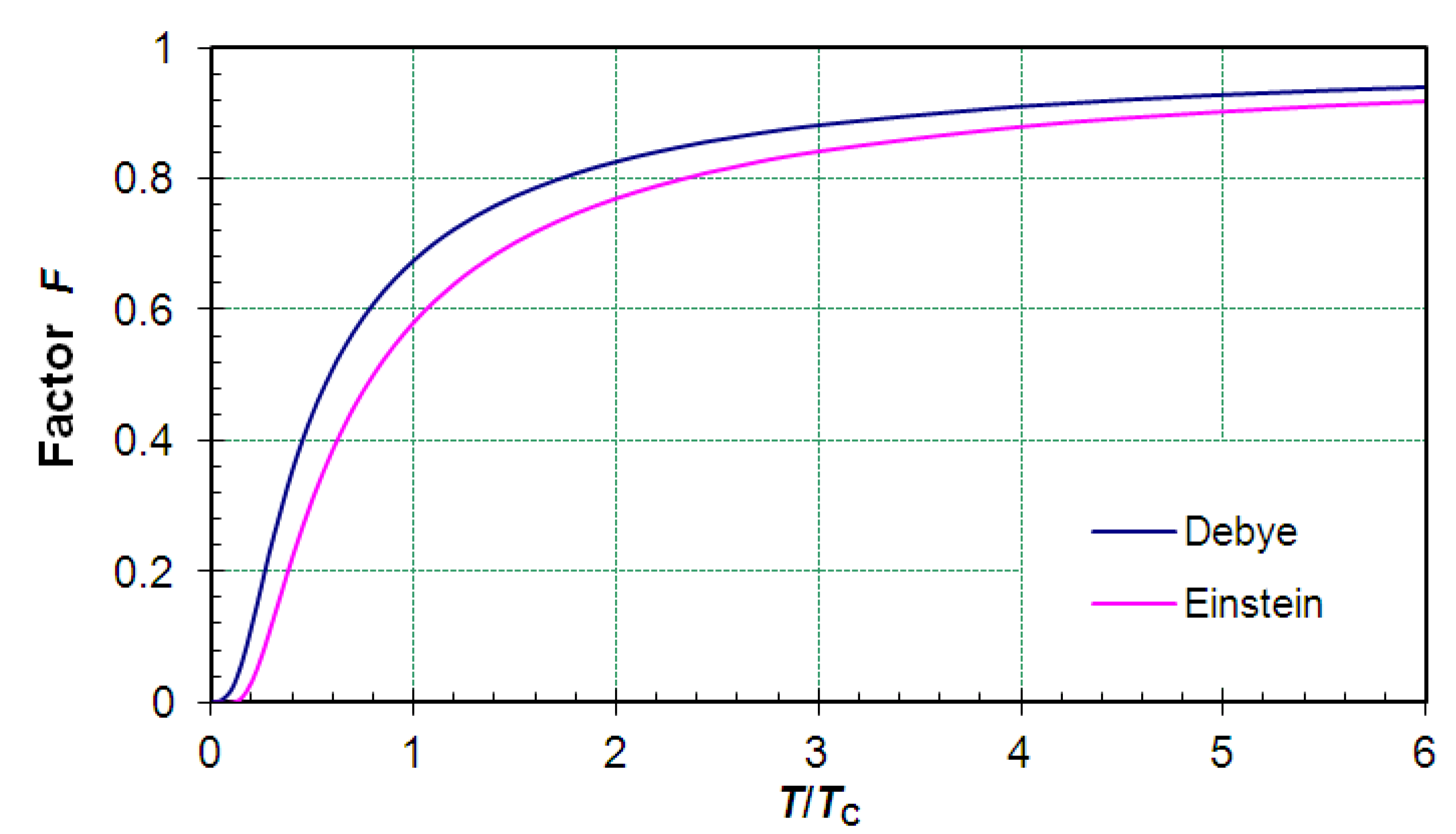
Another departure from classical equipartition emerges in solids at low temperatures by virtue of peculiar quantum effects. The latter can be described with some quantum model, the first of which was Einstein’s single oscillator model, devised in 1907, followed by Nernst-Lindemann’s double oscillator model in 1911 and by Debye’s full spectrum model in 1912. More accurate models have been developed subsequently, based on the vibrational spectrum of the lattice [5,6]. Referring for simplicity to the Einstein and to the Debye model and neglecting zero-point energy, the mean energy of each of the six vibrational atomic degrees of freedom can be expressed in the form ½kT · F, where the factor F ° 1 is a temperature-dependent function, containing the Einstein temperature T_E or the Debye temperature T_D as a parameter [7,8]. The explicit function expression of the factor F depends of course on the model chosen and isn’t of much interest here. It suffices to know that F → 1 for higher temperatures and that F → 0 with falling temperatures. This behaviour is shown in Figure 6.

Figure 6. The diagram below shows the temperature dependence of the factor F, which expresses how much the mean energy of each vibrational degree of freedom of a solid drops below the classical equipartition term ½kT. The graphs are plotted according to the Debye and to the Einstein model. Temperatures range from 0 to 6 T_C, where the characteristic temperature T_C is either the Debye or the Einstein temperature. The function expressions employed were $F(x)=\frac{3}{x^3}{\displaystyle {\int }_0^x\frac{y^3}{e^y-1}dy}$ for the Debye model and $F(x)=\frac{x}{e^x-1}$ for the Einstein model, both with $x=\frac{T_C}{T}$.

Figure 6. The diagram below shows the temperature dependence of the factor F, which expresses how much the mean energy of each vibrational degree of freedom of a solid drops below the classical equipartition term ½kT. The graphs are plotted according to the Debye and to the Einstein model. Temperatures range from 0 to 6 T_C, where the characteristic temperature T_C is either the Debye or the Einstein temperature. The function expressions employed were $F(x)=\frac{3}{x^3}{\displaystyle {\int }_0^x\frac{y^3}{e^y-1}dy}$ for the Debye model and $F(x)=\frac{x}{e^x-1}$ for the Einstein model, both with $x=\frac{T_C}{T}$.

To relate—as in Section 2 and Section 6—entropy with dispersion cardinality, one should start with:

$$\Delta S=\frac{\Delta Q}{T}$$

(13)

and write the transferred heat as:

$$\Delta Q=\frac{1}{2}kT\cdot F\cdot \Delta N$$

(14)

The entropy variation (13) then reduces to:

$$\Delta S=\frac{1}{2}k\cdot F\cdot \Delta N$$

(15)

The entropy variation depends now on F · ΔN instead of on ΔN only. Following the procedure that has already been applied in Section 6, one might call the product F · ΔN, which is always smaller than ΔN, an “effective cardinality” and symbolize it with ΔN*. The last two equations then transform into:

$$\Delta Q=\frac{1}{2}kT\cdot \Delta N*$$

(16)

and:

$$\Delta S=\frac{1}{2}k\cdot \Delta N*$$

(17)

In this way formal agreement with equations (2) and (3) is re-established. Introducing the effective cardinality ΔN*, which is reduced by the factor F compared to the real cardinality ΔN, compensates for the overestimation of the mean energy of the degrees of freedom given by the equipartition term ½kT.

To provide a numerical example, let’s take copper with its Debye temperature 343 K [9]. According to the Debye model, at the earth’s mean surface temperature 300 K the vibrational degrees of freedom of copper atoms share an energy fraction F = 0.6356 of the classical equipartition energy ½kT. Therefore when a heat ΔQ = 1 Joule is transferred to copper at 300 K, it has—according to equation (14)—a dispersion cardinality ΔN = 1,259 µmol. This is significantly more than the corresponding effective dispersion cardinality ΔN* = 800 µmol, which would result if the degrees of freedom of copper atoms could maintain—unaffected by quantum effects—their full classical equipartition energy ½kT. It is the smaller equivalent value 800 µmol that must be taken to determine the entropy variation according to the familiar equation (17).

Utilizing effective cardinalities ΔN*, Figure 1 to Figure 4 can be employed to describe low-temperature systems as well. Figure 3 could e.g., be used to depict the process of “magnetic refrigeration” in a system that comprises both vibrational and magnetic degrees of freedom. Such a system appears to be split into two subsystems, where the degrees of freedom of the magnetic one can be “frozen” applying a strong magnetic field. The removal of the magnetic field allows heat to diffuse from the vibrational subsystem into the magnetic subsystem, thus realizing the mentioned refrigerating effect.

A low-temperature heat engine working according to Figure 4 would have a maximal efficiency that can be found going through once again the steps from equation (4) to equation (7):

$${\eta }_{\max }=\frac{W}{\Delta Q_1}$$

(18)

$${\eta }_{\max }=\frac{\Delta Q_1-\Delta Q_2}{\Delta Q_1}$$

(19)

$${\eta }_{\max }=\frac{\frac{1}{2}k{T}_1\cdot \Delta N*-\frac{1}{2}k{T}_2\cdot \Delta N*}{\frac{1}{2}k{T}_1\cdot \Delta N*}$$

(20)

Reducing the quotient on the right side leads to the expected result:

$${\eta }_{\max }=\frac{T_1-T_2}{T_1}$$

(21)

This is another example of how the application of the conception that heat is spread on dispersion sets leads to consistent results in different areas.

8. Entropy and Efficiency

It can be observed that whenever there is a possibility to increase the associated entropy, this “incites” heat to redistribute inside the system. Hence entropy tends to be maximized. Dispersion sets therefore behave as if they had a built-in “propensity” to increase their cardinality. This provides heat with an internal “drive” to flow against temperature gradients, as shown in Figure 3.

The propensity to increase entropy is also at the basis of the internal “drive” of heat engines. This means that if entropy is not allowed to increase, as in the isentropic process depicted in Figure 4, then there is no stimulus for the process to spontaneously take place. The energetic output per time unit—power—is zero. In order to raise power to useful levels, entropy must be allowed to increase. But if the cardinality of the dispersion set is allowed to increase, less energy is left to be conveyed to the output W and the efficiency promptly falls under its theoretical maximum (7) or (21). Because efficiency falls with increasing power levels, it’s not advisable to demand more power from the motors in our cars—and in other vehicles—than strictly necessary. Power surges should therefore be avoided, pushing the accelerator with gentle care.

A formal treatment of the abovementioned efficiency losses requires some additional assumption. In this regard, in the theory of irreversible processes it is common and useful practice to relate the rate of change of an arbitrary system variable a with the corresponding entropy gradient by a direct proportion:

$$\frac{da}{dt}=C\frac{\partial S}{\partial a}$$

(22)

where C is an appropriate constant [10]. According to this assumption, if the power P delivered by the engine is written in the form:

$$P=\frac{W}{\Delta t}=\eta \frac{\Delta Q_1}{\Delta t}$$

(23)

and if the heat transfer rate ΔQ₁/Δt contained in the above expression is proportional to the entropy increase per unit of heat transferred:

$$\frac{\Delta S}{\Delta Q_1}=\frac{1}{\Delta Q_1}\left(\frac{\Delta Q_2}{T_2}-\frac{\Delta Q_1}{T_1}\right)=\frac{1-\eta }{T_2}-\frac{1}{T_1}$$

(24)

then the above equations combine to:

$$P=\frac{C}{T_2}\left(\frac{T_1-T_2}{T_1}\eta -{\eta }^2\right)$$

(25)

The last equation shows that the power of the engine is a quadratic function of its efficiency η. It has—as it should have—two zero points. The first of these zero points is at η = 0, when no heat is converted into useful work W because the heat flow bypasses the heat engine. The other zero point is at η = η_max, where η_max is given by equations (7) and (21), when the useful work W extracted from the heat flow would be maximal, but the absence of a “drive” given by an entropy increase stops the heat flow itself. Therefore the maximum power is obtained in between these two zero points at:

$$\eta =\frac{1}{2}{\eta }_{\max }$$

(26)

This short calculation suggests that a heat engine may even halve its efficiency when high power levels are demanded. By the way, there is a second reason for avoiding power surges in heat engines: the strong increase in the output of air pollutants. The effect is so pronounced that, should gas turbines be employed instead of hydroelectric power to compensate for sudden variations in wind or solar electric energy supply, this could negatively affect the environmental impact of renewable energy [11].

How does equation (26) apply in practice? As outlined in Section 5, the EPR nuclear power plant under construction in Finland is planned to have a maximal efficiency η_max of 46.5%. The actual thermal efficiency η must however be lower. The manufacturer specifies it to be 37% [12], which is 4/5 of η_max. This is much better than prospected by equation (26). Such a good performance can arguably be expected in virtue of the fact that the EPR—as any other nuclear power plant—is planned to work at a constant production rate, without power surges. It is the latter that may worsen the situation to the point suggested by equation (26).

Figure 7. Finland’s EPR steam turbine system working at the thermal efficiency η = 4/5 η_max = 37% specified by the manufacturer. For an input heat of 1 Joule the dispersion cardinalities are ΔN₁ = 425 µmol and ΔN₂ = 500 µmol. The resulting cardinality increase of 75 µmol per input Joule provides “entropic drive” to the process.

Figure 7. Finland’s EPR steam turbine system working at the thermal efficiency η = 4/5 η_max = 37% specified by the manufacturer. For an input heat of 1 Joule the dispersion cardinalities are ΔN₁ = 425 µmol and ΔN₂ = 500 µmol. The resulting cardinality increase of 75 µmol per input Joule provides “entropic drive” to the process.

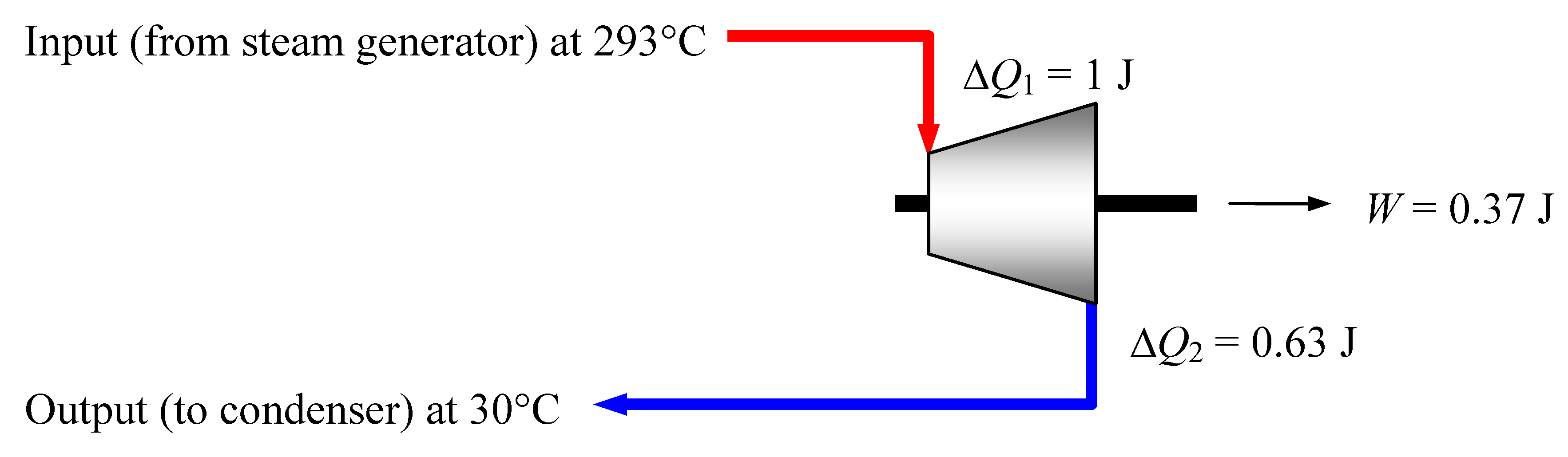
In any case, the calculations for the EPR nuclear power plant made in Section 5 have to be revised, adapting them to the anticipated real efficiency 37%. Thus a heat ΔQ₁ = 1 Joule, delivered to the turbines with a dispersion of ΔN₁ = 425 µmol, will transform—as shown in Figure 7—into an amount W = 0.37 Joule of useful work available at the turbine shaft and into a waste heat ΔQ₂ = 0.63 Joule, spread on ΔN₂ = 500 µmol dispersion elements. The dispersion therefore increases by 75 µmol for every Joule of heat entering the turbine.

9. Results and Discussion

The spreading of heat on a dispersion set made of dispersion elements with the energetic size ½kT, 2.7kT or ½kT · F, which can be understood case-by-case as degrees of freedom subject to equipartition, as radiation quanta or as low-temperature degrees of freedom with quantum properties, gives a vivid representation of how the heat that is transferred to a system induces an entropy change in the system.

Dispersion sets give the heuristic phrase of “heat dispersion” a more precise physical meaning. As shown in this article, they allow describing some of the most basic thermodynamic facts in a simple and straightforward way. The second principle can be pictorially visualized and the efficiency of heat engines is readily deducible with few calculation steps, without previously engaging in lengthy discussions of the Carnot cycle or similar arguments. This could be of some didactic benefit.

The main purpose of this article is to provide “a useful physical picture for understanding entropy” [13]. To this end the small dots in Figure 1 to Figure 4 should be helpful. The big numbers of the involved cardinalities can be conveniently handled converting them in molar form. To facilitate this, the substitutions k ← R and ΔN ← Δn can be introduced in the formalism.

The representation with dispersion sets is possible not only for systems wherein classical equipartition holds, but also for quantized systems that depart from equipartition, provided that they allow the determination of a temperature-dependent mean energy analogous to ½kT. Introducing the “effective cardinality” ΔN* the formalism can be expressed in mechanically equivalent form.

In any case a fundamental constraint remains: dispersion sets are defined within the limits of equilibrium thermodynamics. This means that processes have to take place quasistatically, in order to avoid significant perturbations of the involved systems.

Another aspect to keep in mind is that the representation with dispersion sets aims to provide a model, not a true image of reality. But doesn’t this hold for more refined statistical models as well? The use of dispersion sets avoids complex statistical reasoning and facilitates immediate, “picture aided” logic. Equipartition or other ways to determine mean energy values must however be provided. Where do they come from? They result from a hidden statistical background. Hence representing entropy with dispersion sets is something like a “second-order model”, which is placed on top of the underlying statistical basis. It’s like equipping complex software with a simple graphical user interface, which is easier to use within its restrictions.

10. Conclusions

Though—or just because of—being an instrument of strong simplification, dispersion sets help understanding that dividing ΔQ by T in Clausius’ entropy definition:

$$\Delta S=\frac{\Delta Q}{T}$$

(27)

must not be seen only as a mathematical artifice, justified a posteriori by the useful results that can be drawn from it, but that this operation can per se be attributed a definite physical meaning. In fact, even if “Clausius introduced the concept of entropy, […] without any reference to the microscopic world” [14], it is possible to introduce information about the microscopic world into equation (27) substituting T with ½kT (or a similar mean value) and manipulating the equation accordingly to obtain a number ΔN that counts the elements of a set of degrees of freedom (or quanta) whose energies sum up to ΔQ. Clausius’ definition (27) insists that thermodynamic entropy varies according to this number.

References

- Devine, S. The insights of algorithmic entropy. Entropy 2009, 11, 85–110. [Google Scholar] [CrossRef]
- Pressurized Water Reactor 1600 MWe (EPR)–Nuclear Power Plant Olkiluoto 3, Finland; Framatome ANP GmbH: Erlangen, Germany, 2005; pp. 15–16.
- Baierlein, R. Thermal Physics; Cambridge University Press: Cambridge, UK, 1999; p. 122. [Google Scholar]
- Schrödinger, E. What is Life? Cambridge University Press: Cambridge, UK, 2003; p. 71. [Google Scholar]
- Hulin, M. ’En attendant Debye…’. Eur. J. Phys. 1980, 1, 222–224. [Google Scholar] [CrossRef]
- Westrum, E.F., Jr.; Komada, N. Progress in modeling heat capacity versus temperature morphology. Thermochim. Acta 1986, 109, 11–28. [Google Scholar] [CrossRef]
- Maier, J. Physical Chemistry of Materials: Ions and Electrons in Solids; Wiley: Hoboken, NJ, USA, 2004; pp. 66–68. [Google Scholar]
- Deacon, C.J.; De Bruyn, J.R.; Whitehead, J.P. A simple method of determining Debye temperatures. Am. J. Phys. 1992, 60, 422–425. [Google Scholar] [CrossRef]
- Kestin, J. A Course in Thermodynamics; Hemisphere Publishing Corp.: Washington, DC, USA, 1979; Volume 2, p. 537. [Google Scholar]
- Becker, R. Theorie der Wärme, 3rd ed.; Springer-Verlag: Berlin, Germany, 1985; pp. 315–316. [Google Scholar]
- Katzenstein, W.; Apt, J. Air Emissions Due to Wind and Solar Power. Environ. Sci. Technol. 2009, 43, 253–258. [Google Scholar] [CrossRef] [PubMed]
- Pressurized Water Reactor 1600 MWe (EPR)–Nuclear Power Plant Olkiluoto 3, Finland; Framatome ANP GmbH: Erlangen, Germany, 2005; p. 16.
- Leff, H.S. Thermodynamic entropy: The spreading and sharing of energy. Am. J. Phys. 1996, 64, 1261–1271. [Google Scholar] [CrossRef]
- Tsallis, C.; Gell-Mann, M.; Sato, Y. Extensivity and entropy production. Europhys. News 2005, 36, 186–189. [Google Scholar] [CrossRef]
- Brockhaus contributors; Entropie. In Brockhaus’ Konversations-Lexikon; F. A. Brockhaus: Leipzig, Germany, 1894; Volume 6, pp. 180–181.
© 2010 by the author; licensee Molecular Diversity Preservation International, Basel, Switzerland. This article is an open-access article distributed under the terms and conditions of the Creative Commons Attribution license (http://creativecommons.org/licenses/by/3.0/).
Share and Cite
MDPI and ACS Style
Kolarczyk, B. Representing Entropy with Dispersion Sets. Entropy 2010, 12, 420-433. https://doi.org/10.3390/e12030420
AMA Style
Kolarczyk B. Representing Entropy with Dispersion Sets. Entropy. 2010; 12(3):420-433. https://doi.org/10.3390/e12030420
Chicago/Turabian StyleKolarczyk, Bernhard. 2010. "Representing Entropy with Dispersion Sets" Entropy 12, no. 3: 420-433. https://doi.org/10.3390/e12030420