Entropy-Based Method of Choosing the Decomposition Level in Wavelet Threshold De-noising

Abstract

In this paper, the energy distributions of various noises following normal, log-normal and Pearson-III distributions are first described quantitatively using the wavelet energy entropy (WEE), and the results are compared and discussed. Then, on the basis of these analytic results, a method for use in choosing the decomposition level (DL) in wavelet threshold de-noising (WTD) is put forward. Finally, the performance of the proposed method is verified by analysis of both synthetic and observed series. Analytic results indicate that the proposed method is easy to operate and suitable for various signals. Moreover, contrary to traditional white noise testing which depends on “autocorrelations”, the proposed method uses energy distributions to distinguish real signals and noise in noisy series, therefore the chosen DL is reliable, and the WTD results of time series can be improved.

1. Introduction

This paper considers the problem of de-noising in the domains of applied research and engineering activities, such as business, medicine, physics, earth sciences and hydraulic engineering. De-noising is a substantial issue in time series analysis because noise has a great influence on the real characteristics of time series [1,2,3,4]. Observed time series in nature usually show non-stationary and multi-temporal scale characteristics. However, the traditional de-noising methods used presently are mainly based on model simulation or spectral analysis, and they cannot reveal these complicated characteristics of series and thus cannot satisfactorily meet practical needs [5,6,7,8]. Compared with them, the wavelet threshold de-noising (WTD) method is more effective and is especially applicable in various engineering activities, because it can elucidate the localized characteristics of non-stationary time series both in the temporal and frequency domains [9,10,11,12]. Although being theoretically powerful, in practice the WTD method is influenced by four basic but key issues, namely the choice of wavelet, the choice of decomposition level (DL), threshold estimation and choice of thresholding rules, respectively [13]. Many studies have been conducted in various fields to develop the WTD method. For example, Coifmain and Wickerhauser proposed algorithms based on Shannon entropy for best basis selection, which permit efficient compression of signals [14]; Berger et al. described applications of de-noising algorithms for removing noise from music [15] mainly based on the studies in [14]; Lou and Hu proposed an approach to suppress non-stationary wideband noise based on the dyadic wavelet transform and the simplified Karhunen-Loeve transform [16]; Dimoulas et al. designed de-noising algorithms based on the Wiener filtering technique, and further compared the results obtained by using various decomposition schemes, different mother wavelets and various thresholding options [17].

The authors have reviewed traditional de-noising methods and the wavelet-based de-noising methods in [13]. Three of their main defects were summarized; they are the probability description of noise, the accuracy of threshold estimation methods and the validity of thresholding rules, respectively. Then, the key issues of WTD except the choice of DL were discussed, and approaches to solve them based on entropy theory were put forward. After that, an improved WTD method was proposed, whose basic idea is to estimate proper thresholds and further to determine the accurate de-noising results according to the variations of de-noised series’ complexities and separated noise’s random characters, which are characterized by the wavelet energy entropy (WEE) and principle of maximum entropy (POME), respectively. Finally, analytic results of both synthetic and observed series verified the performance of the improved WTD method. To the authors’ knowledge, the issue of choice of decomposition level in WTD is little discussed, whether in [13] or in other studies, and no effective and operable approaches could be followed presently.

In this study, the main objective is to put forward a method of choosing the decomposition level to develop the WTD method. Moreover, the proposed method is also based on the wavelet energy entropy to keep in step with the analytic process of WTD in [13]. To achieve this purpose, in Section 2, the WTD method is briefly introduced, and then the energy distributions of noises following various probability distributions are described using WEE, based on which the method of choosing DL is proposed. In Section 3, we verify the performance of the proposed method by doing case studies, and analytic results indicate that de-nosing results can be improved by using the proposed method. Finally, this study is summarized and concluded in the last section.

2. The Proposed Method of Choosing the Decomposition Level

2.1. Wavelet Threshold De-noising

The process of wavelet threshold de-noising (WTD) is based on discrete wavelet transform (DWT), especially the dyadic DWT commonly used in practice [18]. The dyadic DWT consists of log₂n stages at most given the analyzed series with the length of n. The first stage starts from original series, and the results include two types of wavelet coefficients sets as “approximations” and “details” under each level. In each except the first stage, only approximation coefficients are analyzed.

When we obtain the details wavelet coefficients W_j,k of DWT, a proper threshold T_j can be first estimated and then used to adjust W_j,k under each level j according to Equation (1) [5,19,20]:

$$W{\text{'}}_{j,k}=\rho (W_{j,k},T_j)$$

(1)

in which ρ() is the thresholding rule, such as hard-, soft-, mid-thresholding rules and Wiener thresholding. W’_j,k is the adjusted value of W_j,k. Finally, the de-noised series can be reconstructed by using the adjusted W’_j,k, and the difference between de-noised and original series is the separated noise. There are four key issues in the WTD process, the first two are the choice of wavelet and DL which determine the accuracy of DWT results; the last two are the estimation of thresholds and choice of thresholding rules.

2.2. Autocorrelations and Energy Distributions of Noises

In present engineering activities, the decomposition level in WTD is usually chosen by the white noise testing method [21]. Its idea is to first separate noisy series into sub-signals under different levels and then analyze their autocorrelations; once a certain sub-signal cannot pass the white noise testing, the corresponding level is thought as the best result. However, noise usually generates auto-correlated sub-signals, as shown in Table 2, and we cannot easily differentiate whether they are real deterministic signals or just pseudo deterministic signals caused by noise. Therefore, the white noise testing is invalid and its results are inaccurate and unreliable in many practical situations.

Table 1. Probability distributions used to generate noises in this paper.

Type	Expression	Parameters
Normal	$f(x)=\frac{1}{\sqrt{2\pi }\sigma }\exp (-\frac{{(x-\mu )}^2}{{\sigma }^2})$	μ, σ
Lognormal	$f(x)=\frac{1}{x\sqrt{2\pi }{\sigma }_y}\exp (-\frac{{(\ln x-{\mu }_y)}^2}{{{\sigma }_y}^2})$	μy, σy
Pearson-III	$f(x)=\frac{{\beta }^{\alpha }}{\Gamma (\alpha )}{(x-a_0)}^{\alpha -1}\exp (-\beta (x-a_0))$	α, β, a0

Table 1. Probability distributions used to generate noises in this paper.

Type	Expression	Parameters
Normal	$f(x)=\frac{1}{\sqrt{2\pi }\sigma }\exp (-\frac{{(x-\mu )}^2}{{\sigma }^2})$	μ, σ
Lognormal	$f(x)=\frac{1}{x\sqrt{2\pi }{\sigma }_y}\exp (-\frac{{(\ln x-{\mu }_y)}^2}{{{\sigma }_y}^2})$	μy, σy
Pearson-III	$f(x)=\frac{{\beta }^{\alpha }}{\Gamma (\alpha )}{(x-a_0)}^{\alpha -1}\exp (-\beta (x-a_0))$	α, β, a0

Differing from the white noise testing, the proposed method of choosing the DL in the following is based on the difference of energy distributions between real signals and noise. To orderly state these contents and to clearly explain the proposed method, we first analyze the autocorrelations and energy distributions of noises by doing Monte-Carlo (MC) tests. The number of MC tests is 100,000 to make the results stable. According to practical engineering situations, all the noises which follow normal, lognormal and Pearson-III distributions in Table 1 are analyzed to ensure the reasonability and credibility of the conclusions. In dyadic DWT process of noise, the “coif5” wavelet is used as example considering that the results by different wavelets are just the same, and the theoretical maximum M of DL is calculated as:

$$M=[{\log }_2(n_{f(t)})]$$

(2)

where [∙] means taking the integer part of real value in square bracket. n_f(t) is the length n of series f(t). Because all the generated noise series have the same length of 1,000, the calculated M is 9. Dyadic DWT noise results include the approximation coefficients under one level and the details coefficients under nine levels. The latter is focused on in this study because we want to provide useful suggestions for WTD.

First, we reconstruct the sub-signals of noises under nine levels, and calculate the lag-1 autocorrelation coefficient R₁ and energy E by Equation (3):

$$\begin{array}{c}{R}_1(j)=\frac{{\displaystyle \sum _{t=1}^{n-1}(f_j(t)-\overline{f_j}(t))(f_j(t+1)-\overline{f_j}(t))}}{{\displaystyle \sum _{t=1}^n{(f_j(t)-\overline{f_j}(t))}^2}}\\ E_j={\displaystyle \sum _{t=1}^n{(f_j(t))}^2}\end{array}$$

(3)

where n is the series’ length, and t is the data number. $\overline{f_j}(t)$ is the mean of the sub-signal f_j(t) under the DL j. The means of MC results are depicted in Figure 1 and summarized in Table 2.

Figure 1. The lag-1 autocorrelation coefficient R₁ and energy E of sub-signals of various noises under different decomposition levels (DLs).

Figure 1. The lag-1 autocorrelation coefficient R₁ and energy E of sub-signals of various noises under different decomposition levels (DLs).

Table 2. Calculation results of the lag-1 autocorrelation coefficient R₁ and energy E of sub-signals of various noises under different decomposition levels (DLs).

Type	Index	Decomposition level (DL)
		1	2	3	4	5	6	7	8	9
Normal	R1	−0.611	0.331	0.806	0.948	0.987	0.995	0.997	0.999	0.999
	E	499.59	249.87	125.29	62.64	30.95	17.30	12.21	7.24	5.86
Lognormal	R1	−0.612	0.332	0.806	0.948	0.987	0.996	0.998	0.999	0.999
	E	499.50	249.42	125.15	62.70	30.91	17.24	11.94	7.09	5.70
Pearson-III	R1	−0.611	0.331	0.806	0.948	0.987	0.996	0.997	0.999	0.999
	E	499.45	250.21	124.89	62.61	30.97	17.44	12.14	7.32	5.83

Table 2. Calculation results of the lag-1 autocorrelation coefficient R₁ and energy E of sub-signals of various noises under different decomposition levels (DLs).

Type	Index	Decomposition level (DL)
		1	2	3	4	5	6	7	8	9
Normal	R1	−0.611	0.331	0.806	0.948	0.987	0.995	0.997	0.999	0.999
	E	499.59	249.87	125.29	62.64	30.95	17.30	12.21	7.24	5.86
Lognormal	R1	−0.612	0.332	0.806	0.948	0.987	0.996	0.998	0.999	0.999
	E	499.50	249.42	125.15	62.70	30.91	17.24	11.94	7.09	5.70
Pearson-III	R1	−0.611	0.331	0.806	0.948	0.987	0.996	0.997	0.999	0.999
	E	499.45	250.21	124.89	62.61	30.97	17.44	12.14	7.32	5.83

To continue, we use the wavelet energy entropy (WEE) to describe the variation of the degrees of complexity of noise with DLs. Specifically, we use each value M_i of the DLs from 1 to 9 and apply dyadic DWT to the noise series, then reconstruct the sub-signal under each level. Finally, we calculate the value of WEE by Equation (4):

$$\begin{array}{l}WEE(i)=-{\displaystyle \sum _{j=1}^{M_i}{P}_j\ln P_j}with\\ P_j=E_j/{\displaystyle \sum _{j=1}^{M_i}{E}_j={\displaystyle \sum _{t=1}^n{(f_j(t))}^2}/{\displaystyle \sum _{j=1}^{M_i}({\displaystyle \sum _{t=1}^n{(f_j(t))}^2})}}{M}_i=1,\cdots ,M\end{array}$$

(4)

The WEE is defined according to the information entropy theory [22], whose value quantitatively reflects the series’ complexities. The bigger the value of WEE is, the more complicated the series is, and vice versa [23]. The analytic results of WEE of noises are depicted in Figure 2.

Analytic results in Table 2 and Figure 1 indicate that the R₁ values of noises’ sub-signals increase from the starting value of −0.611 to the end value of 0.999 with the increasing DL. Except the R₁ of 0.331 under the DL 2, all the absolute values of R₁ of noises’ sub-signals under other DLs are bigger than 0.5. This indicates that the sub-signals of noises have good autocorrelations. Therefore, when we choose DL according to the “autocorrelations”, the results are unreasonable and unreliable in many practical cases. Furthermore, when we set the DL to be 9, Figure 1 shows that the energy of noises is mainly concentrated in small temporal scales, and it exponentially decreases with DL with the base of 2, which is due to the grid of dyadic DWT. Besides, Figure 2 displays that the value of WEE increases with the DL, so the degree of complexity of noise can be revealed and presented guardedly, and it obtains the maximum when using the DL 9. Finally, it can be found that for these noises which follow normal, lognormal and Pearson-III distributions, their energy distributions (both the values of E and WEE) are similar to each other. This conclusion is very favorable to the choice of DL as discussed in the following.

Figure 2. Values of wavelet energy entropy (WEE) of various noises when analyzed by using different decomposition levels (DLs).

Figure 2. Values of wavelet energy entropy (WEE) of various noises when analyzed by using different decomposition levels (DLs).

2.3. The Method Proposed

According to the discussed energy distributions of noises results, we propose a method for choice of the decomposition levels in WTD. To clearly describe it, we first define the X, S, S^~ and N as the noisy series (or original series), real series, de-noised series and noise, respectively. Theoretically speaking, when we apply dyadic DWT to the noisy series X, the energies of real series S in X are concentrated on several DLs corresponding to the deterministic components (e.g., periods, trend) of X [24], but the energy of noise N scatters in the whole temporal scales and rapidly decays with DLs as discussed in Section 2.2. Therefore, when we initially use a certain small DL and apply dyadic DWT to the analyzed noisy series X, the sub-signals reconstructed by using details wavelet coefficients are mainly composed of noise, so the WEEs of X and those of N should be similar. Along with the increasing of DLs and once reaching to certain value of DL^*, the real series S in X can be identified for the first time. In this case, the WEE of X would be obviously different from that of N. However, if we use the DL^* or increase DL again, several real signals would be removed in the process of WTD, which are clearly shown in the latter examples. Therefore, the chosen DL should be DL^* less 1, and then the de-noised series S^~ can be obtained by WTD method.

The analytic steps by the proposed method are depicted in Figure 3 and also explained as follows:

(1)

For the noisy series X analyzed, we first calculate the theoretical maximum M of DL by Equation (2), and normalize it by Equation (5):

$$X=\frac{(X-\overline{X})}{\sigma (X)}$$

(5)

in which $\overline{X}$ and $\sigma (X)$ are the mean and standard deviation of X, respectively.

(2)

Then, we apply dyadic DWT to X by using each value of the DLs from 1 to M, and calculate the values of WEE by Equation (4), based on which we obtain the WEE curve of X.

(3)

According to the practical situations and experiences, we choose an appropriate probability distribution to generate “normalized” noise series with the same length as that of X. Then we determine the WEE curve of noise by doing Monte-Carlo tests.

(4)

Finally, we compare the values of WEE of the noisy series X with those of noise with the increasing of DLs. Once the value of WEE of X is obviously different from that of noise under certain DL^*, the best DL can be chosen as DL^* less 1. Besides, the differential coefficient of WEE in Equation (6) can be used together to compare the WEEs of noisy series X and noise, because it is an extreme value under the DL^* and can reflect their difference more clearly;

$$D(j)=\frac{d(WEE)}{d(DL)}=\frac{WEE(j)-WEE(j-1)}{j-(j-1)}=WEE(j)-WEE(j-1)$$

(6)

where D(j) is the differential coefficient of WEE under the DL j, d(∙) means the derivation calculus.

Figure 3. Steps of choosing suitable decomposition level (DL) in the process of wavelet threshold de-noising by using the proposed method.

Figure 3. Steps of choosing suitable decomposition level (DL) in the process of wavelet threshold de-noising by using the proposed method.

As described above, the proposed method of choosing DL in WTD is based on the difference of energy distributions between noisy series and noise, thus it has dependable physical basis and can accurately make out the real and pseudo deterministic sub-signals in noisy series. Moreover, differing from other wavelet-based de-noising methods which generally need to previously know some inaccessible prior-information [5,6,7,8,14,15,16,17,8,14], the proposed method just needs to choose proper probability distribution to generate noise. Whereas this need is not crucial in practice, because the analytic results by using different types of noises are just the same.

3. Case Studies

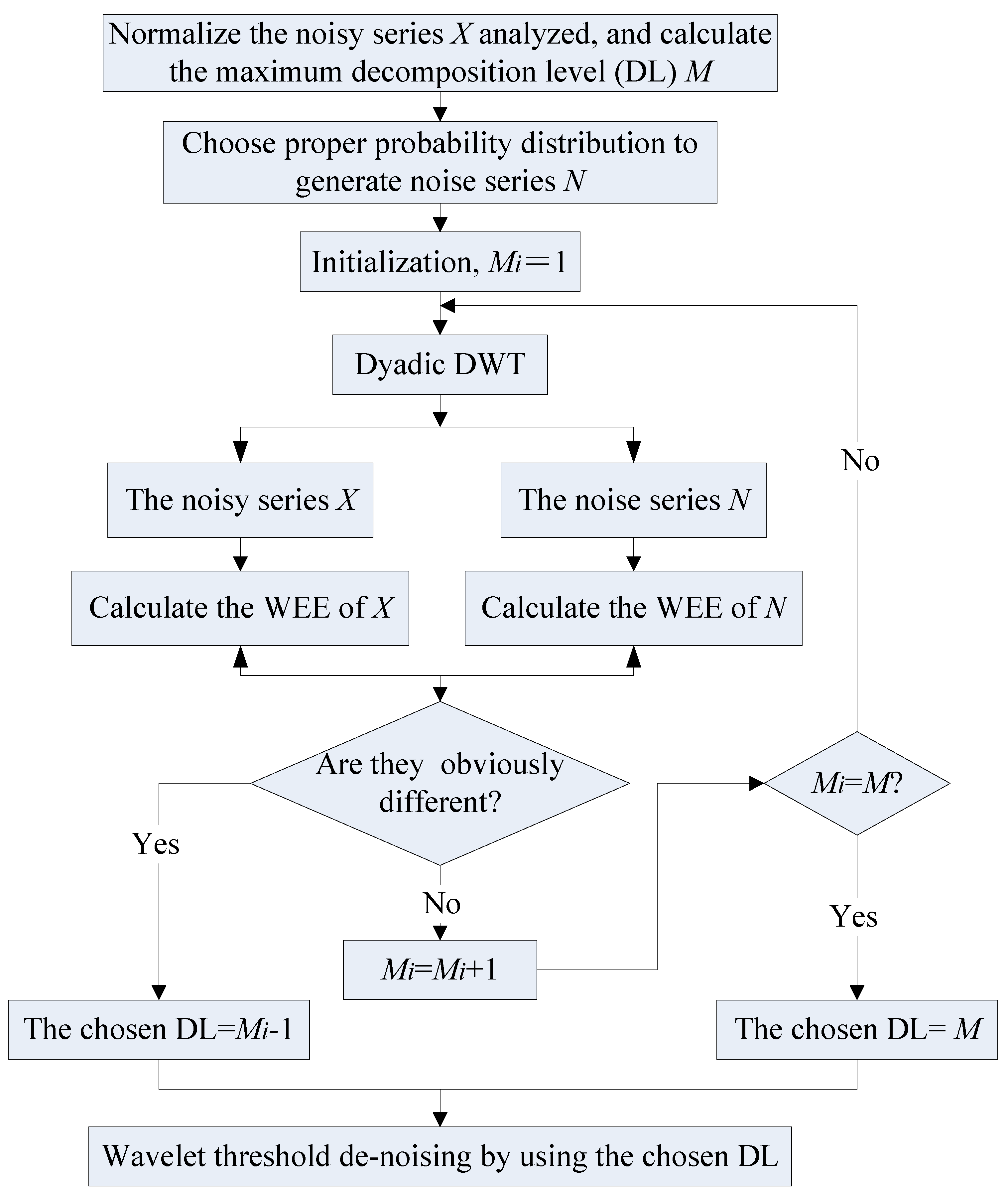
Both synthetic series and observed series data are analyzed here to verify the performance of the proposed method. All of them are also analyzed by the white noise testing method for comparison. Other wavelet-based de-noising methods are not included here, considering that they have been discussed and compared with the entropy-based WTD method in [13]. Moreover, three quantitative indexes, SNR (signal-to-noise ratio), MSE (mean square error) and R_xy (lag-0 cross-correlation coefficient) in Equation (7), are used to judge the accuracy of de-noising results obtained by using different DLs, mainly to ensure the soundness of conclusions. 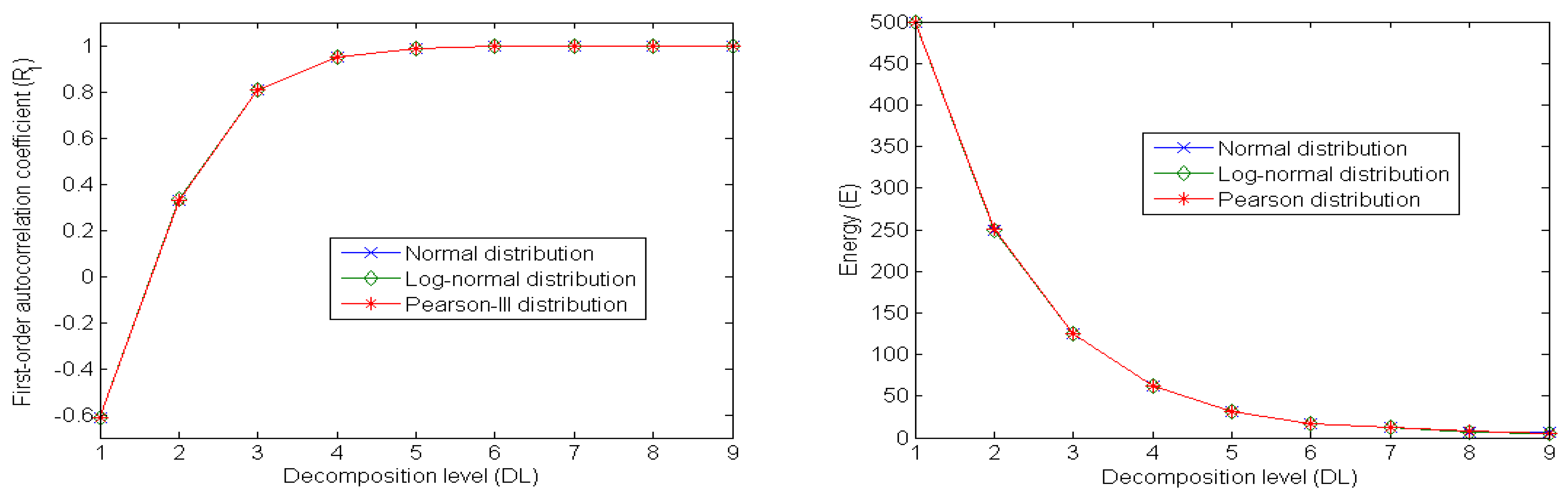Besides, the wavelet variance estimator is also used to compare these different de-noising results [23]. Because the energy distributions of various noises are just the same, the normally distributed noise is used here;

$$\begin{array}{c}SNR=-10\times \log (Var(N)/Var(S^{~}))\\ MSE=Var(S-S^{~})\\ R_{xy}(0)=\frac{{\displaystyle \sum _{t=1}^n(S-\overline{S})(S^{~}-{\overline{S}}^{~})}}{\sqrt{{\displaystyle \sum _{t=1}^n{(S-\overline{S})}^2}}\sqrt{{\displaystyle \sum _{t=1}^n{(S^{~}-{\overline{S}}^{~})}^2}}}\end{array}$$

(7)

in which $\overline{S}$ and ${\overline{S}}^{~}$ is the mean of real series S and the de-noised series S^~ respectively, and N is the separated noise. Var() means calculating the variance.

3.1. Synthetic Series Analysis

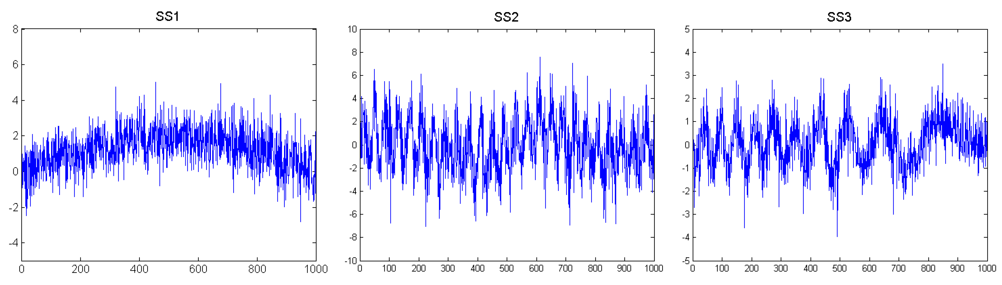
Three synthetic series are generated by the Monte-Carlo method and are shown in Figure 4.

Figure 4. Three synthetic series data used in this paper.

Figure 4. Three synthetic series data used in this paper.

Among them, the SS1 series has first an upward and then a downward trend, the SS2 series has two periods of 100 and 500; whereas the SS3 series has a damped period. Their real values of SNR are −9.562, −4.012 and −3.365 respectively. Considering that the noise-contaminated degrees of them are serious, we deem that the proposed method is effective provided that it is suitable for the three synthetic series.

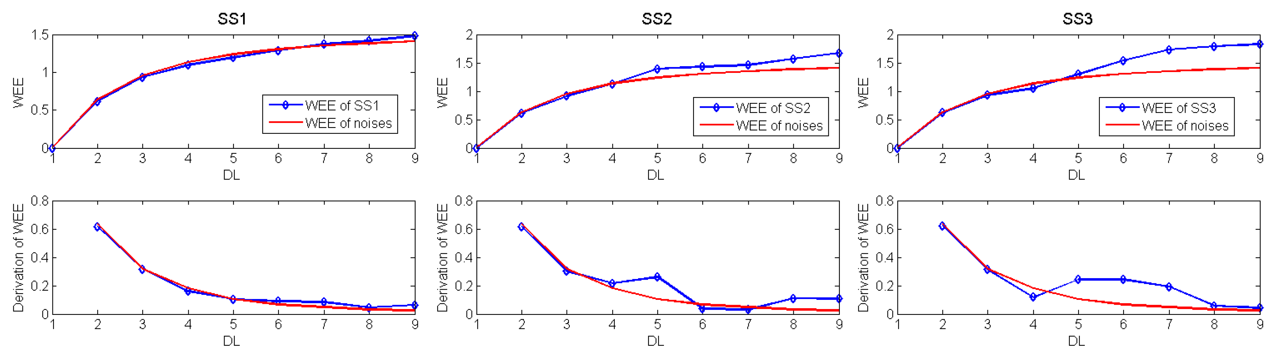
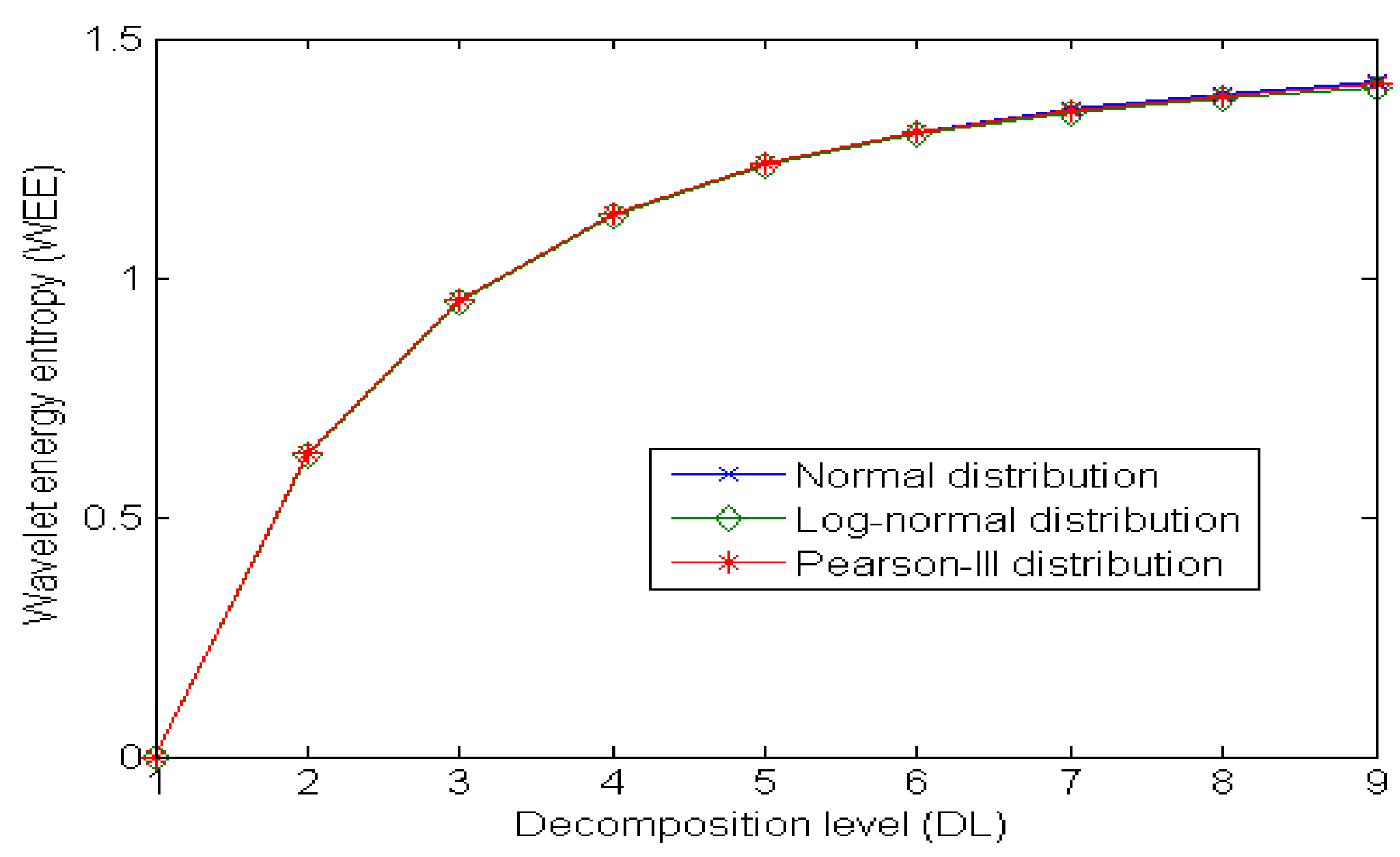
Each of the three synthetic series is analyzed by the proposed method using the “coif5” wavelet. The calculated WEE curves of them are depicted in Figure 5. Furthermore, they are de-noised by the WTD method in [13] using different DLs. The calculation results of SNR, MSE and R_xy are summarized in Table 3, and the wavelet variance curves of these de-noised series obtained by using different DLs are presented in Figure 6.

Figure 5. Values of WEE of three synthetic series and the corresponding derivation coefficients when analyzed by using different decomposition levels (DLs).

Figure 5. Values of WEE of three synthetic series and the corresponding derivation coefficients when analyzed by using different decomposition levels (DLs).

Table 3. De-noising results of three synthetic series by using different decomposition levels (DLs).

Series	Index	Real value	Decomposition level (DL)
			1	2	3	4	5	6	7	8	9
SS1	SNR	-9.562	4.844	-2.121	-5.543	-7.466	-8.310	-9.383	-9.581	-9.530	-9.545
	MSE		0.469	0.236	0.121	0.065	0.040	0.013	0.005	0.004	0.010
	Rxy		0.665	0.782	0.870	0.922	0.949	0.983	0.993	0.995	0.987
SS2	SNR	-4.012	7.054	0.954	-1.833	-3.983	-18.58	-19.18	-19.67	-25.38	-29.27
	MSE		1.708	0.839	0.417	0.387	1.500	1.481	1.458	1.59	1.611
	Rxy		0.760	0.858	0.921	0.921	0.640	0.650	0.661	0.660	0.706
SS3	SNR	-3.365	7.867	1.811	-1.048	-1.792	-4.525	-10.46	-17.82	-19.45	-19.53
	MSE		0.305	0.146	0.067	0.046	0.074	0.158	0.191	0.211	0.224
	Rxy		0.775	0.871	0.934	0.953	0.918	0.817	0.817	0.794	0.768

Table 3. De-noising results of three synthetic series by using different decomposition levels (DLs).

Series	Index	Real value	Decomposition level (DL)
			1	2	3	4	5	6	7	8	9
SS1	SNR	-9.562	4.844	-2.121	-5.543	-7.466	-8.310	-9.383	-9.581	-9.530	-9.545
	MSE		0.469	0.236	0.121	0.065	0.040	0.013	0.005	0.004	0.010
	Rxy		0.665	0.782	0.870	0.922	0.949	0.983	0.993	0.995	0.987
SS2	SNR	-4.012	7.054	0.954	-1.833	-3.983	-18.58	-19.18	-19.67	-25.38	-29.27
	MSE		1.708	0.839	0.417	0.387	1.500	1.481	1.458	1.59	1.611
	Rxy		0.760	0.858	0.921	0.921	0.640	0.650	0.661	0.660	0.706
SS3	SNR	-3.365	7.867	1.811	-1.048	-1.792	-4.525	-10.46	-17.82	-19.45	-19.53
	MSE		0.305	0.146	0.067	0.046	0.074	0.158	0.191	0.211	0.224
	Rxy		0.775	0.871	0.934	0.953	0.918	0.817	0.817	0.794	0.768

Figure 6. Wavelet variance curves of the de-noised synthetic series obtained by using different decomposition levels (DLs).

Figure 6. Wavelet variance curves of the de-noised synthetic series obtained by using different decomposition levels (DLs).

The analytic results in Figure 5 indicate that the chosen DLs are different for the three synthetic series with different real signals. Concretely, the WEEs of SS1 series are very close to those of noise under the DLs from 1 to 8, whereas the sub-signal under the DL 9 is part of the trend of SS1 series, so its WEE has big difference with that of noise. The WEEs of SS2 series and noise are very similar under the DLs from 1 to 4; but they show obvious differences under the DL 5 and the value of D(5) is an extreme value, because the sub-signal of SS2 series under the DL 5 corresponds to the period of 200. As for SS3 series, its WEEs are close to those of noise before the DL 4, but they are obviously different under the DL 5 and the value of D(5) is also an extreme value. Furthermore, analytic results in Table 3 show that de-noising results of these synthetic series vary with the DL used. To be specific, the de-noising result of SS1 series by using the DL 8 is the best, because the MSE with the value of 0.004 is the smallest, the R_xy with the value of 0.995 is the biggest, and the calculated SNR of −9.530 is very close to the real SNR of −9.562. For SS2 series, the values of SNR, MSE and R_xy under the DL 4 are −3.983, 0.387 and 0.921 respectively, all of which are the best results among those under different DLs; and for SS3 series, the SNR, MSE and R_xy of −1.792, 0.046 and 0.953 under the DL 4 are also the best results among those under different DLs. 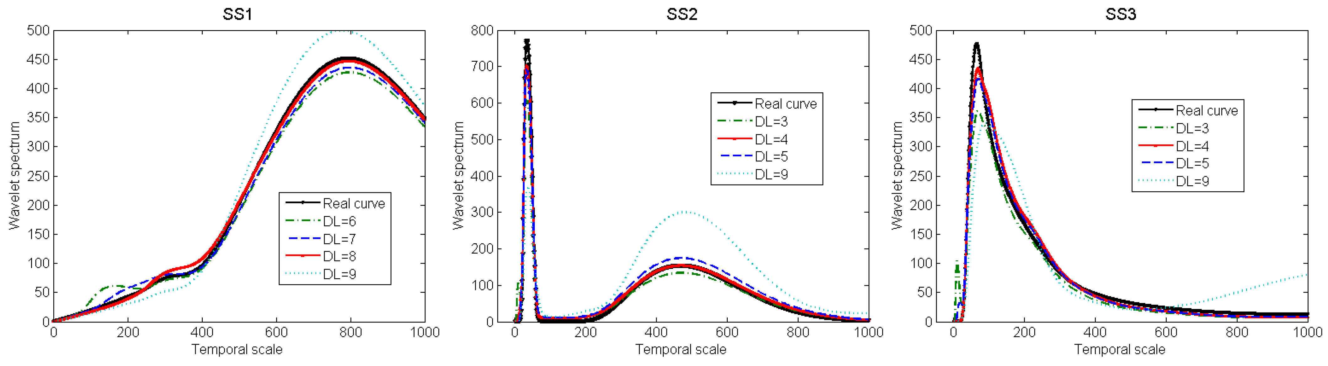Besides, Figure 6 on one hand shows the same conclusions as those in Table 3; on the other hand, it shows that the wavelet variance curves of de-noised series reflect irregular fluctuations under small temporal scales when using the smaller DLs, which means that noise is not removed completely; whereas the de-noised series’ wavelet spectral densities under small scales are smaller than the real values when using the bigger DLs, which means that several real signals are removed. 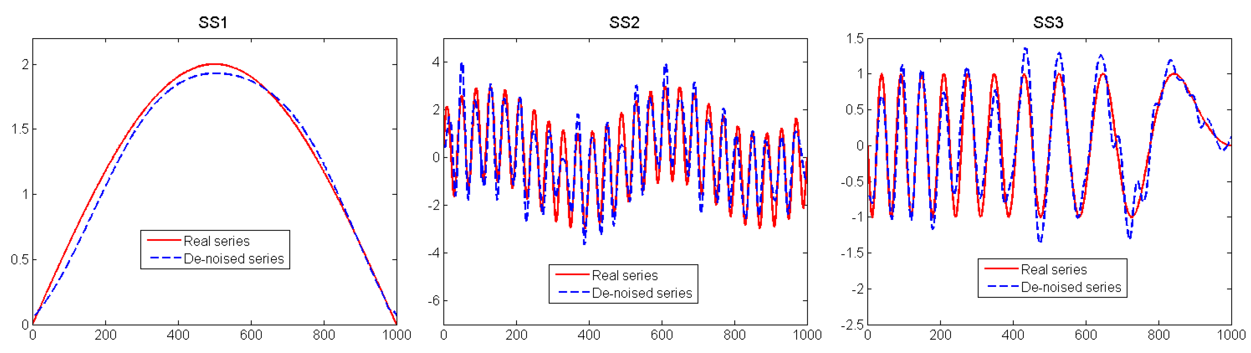As a result, all the results in Figure 5, Figure 6 and Table 3 show the same conclusion: the chosen DLs for the three synthetics series are 8, 4 and 4 respectively. Finally, these synthetic series are de-noised by using the chosen DLs, and the results are presented in Figure 7.

Figure 7. De-noising results of the three synthetic series by using the chosen decomposition levels (DLs).

Figure 7. De-noising results of the three synthetic series by using the chosen decomposition levels (DLs).

In addition, the lag-1 autocorrelation coefficient R₁ of the sub-signals of these synthetic series under different levels is calculated, and the results are listed in Table 4. It indicates that no matter which synthetic series is analyzed, their sub-signals under different DLs cannot pass the white noise testing, because the smallest absolute value of the R₁ of them is 0.326, 0.326 and 0.341, respectively under the DL 2. Therefore, it can be further concluded that analytic results by the proposed method are more reliable.

Table 4. Calculation results of the lag-1 autocorrelation coefficient R₁ of the sub-signals of synthetic series under different decomposition levels (DLs).

Series		Decomposition level (DL)
	1		2	3	4	5	6	7	8	9
SS1	-0.646		0.326	0.804	0.940	0.990	0.998	0.998	0.996	1.000
SS2	-0.579		0.326	0.810	0.949	0.990	0.996	0.999	0.999	0.998
SS3	-0.642		0.341	0.814	0.937	0.987	0.994	0.996	0.999	0.998

Table 4. Calculation results of the lag-1 autocorrelation coefficient R₁ of the sub-signals of synthetic series under different decomposition levels (DLs).

Series		Decomposition level (DL)
	1		2	3	4	5	6	7	8	9
SS1	-0.646		0.326	0.804	0.940	0.990	0.998	0.998	0.996	1.000
SS2	-0.579		0.326	0.810	0.949	0.990	0.996	0.999	0.999	0.998
SS3	-0.642		0.341	0.814	0.937	0.987	0.994	0.996	0.999	0.998

3.2. Observed Series Analysis

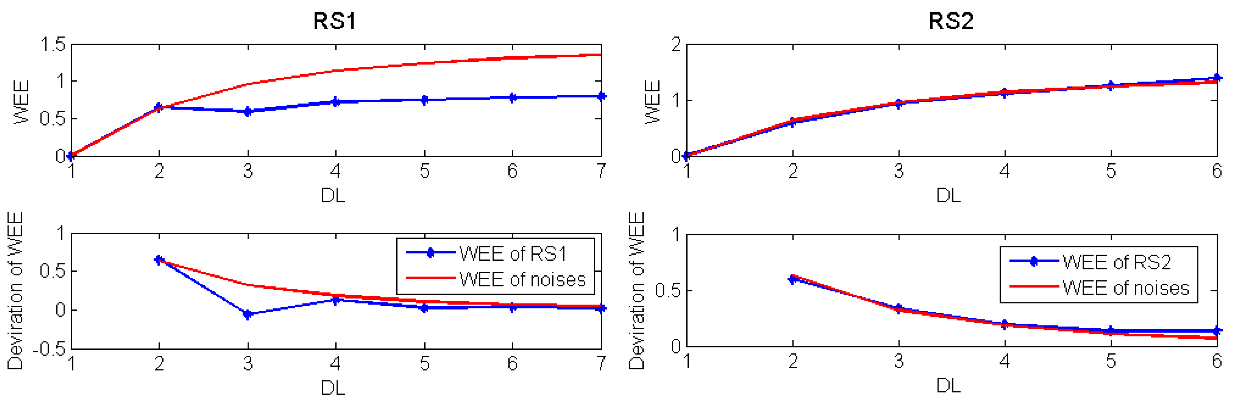
Two observed hydrologic series, RS1 and RS2, are analyzed here to further verify the performance of the proposed method. Among them, RS1 presents 20 years (1978–1997) of monthly runoff series measured at the Dashankou hydrologic station at Kaidu River in the northwest of China, and it has two obvious periods of about 6 months and 12 months [4]. RS2 presents 125-day rainfall series (June 1 to October 3 in 2003) measured in Hanqiao Coal Mine located in the mid-eastern of China [25].

The two series are analyzed by using the “dmey” and “db6” wavelets, respectively [4,25]. Their WEE curves are shown in Figure 8. Then, they are de-noised and the results are presented in Figure 9 and Table 5. Besides, analytic results by the white noise testing method are listed in Table 6.

Figure 8. Values of WEE of the two observed series and the corresponding derivation coefficients when analyzed by using different decomposition levels (DLs).

Figure 8. Values of WEE of the two observed series and the corresponding derivation coefficients when analyzed by using different decomposition levels (DLs).

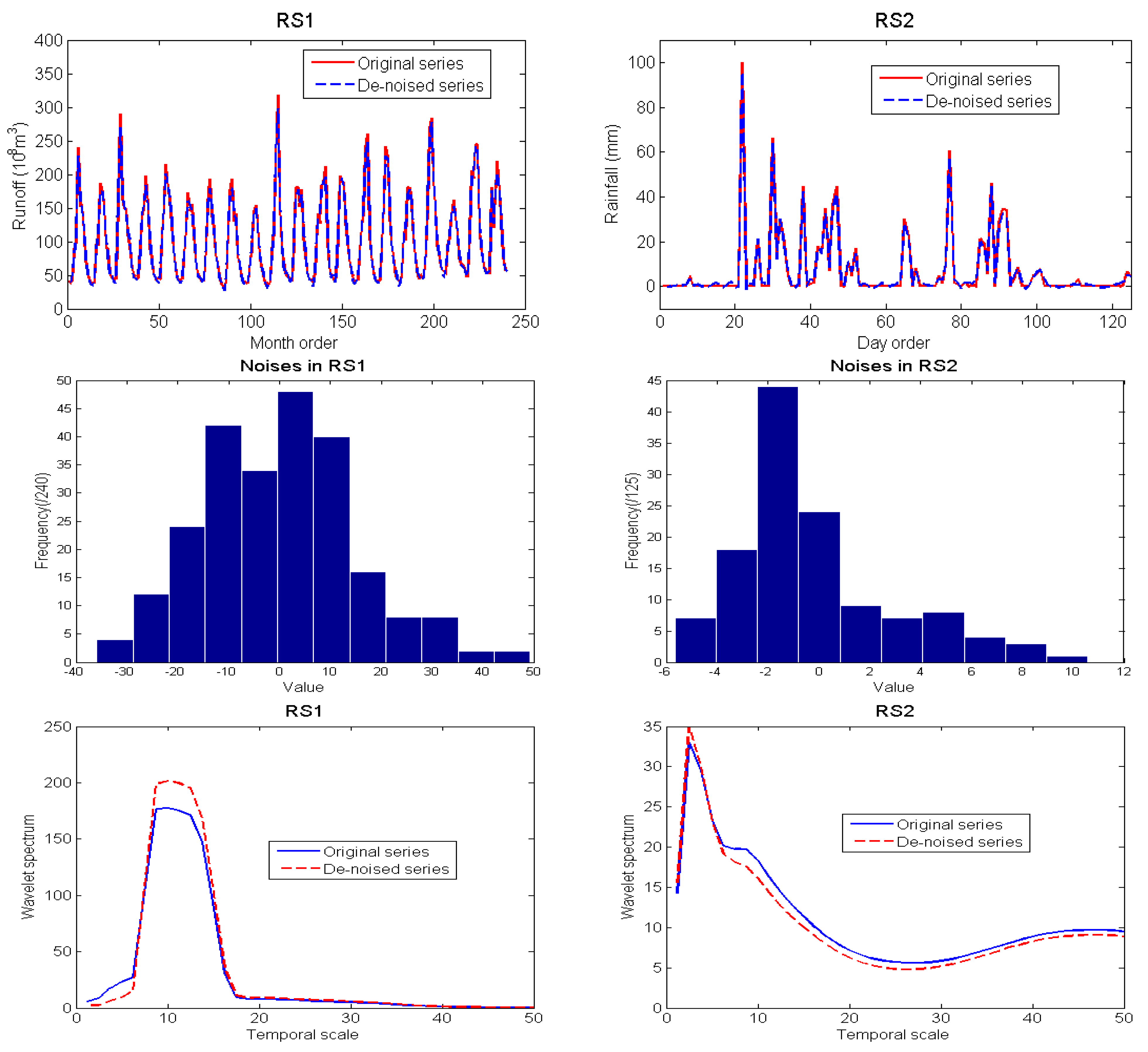
Figure 9. De-noising results of the two observed series by using the chosen decomposition levels (DLs) (upper), histograms of the separated noise (mid) and the wavelet variance curves of the de-noised series and observed series data (lower).

Figure 9. De-noising results of the two observed series by using the chosen decomposition levels (DLs) (upper), histograms of the separated noise (mid) and the wavelet variance curves of the de-noised series and observed series data (lower).

Table 5. Calculated values of SNR of the two de-noised observed series data by using different decomposition levels (DLs).

Series	Decomposition level (DL)
	1	2	3	4	5	6	7
RS1	30.904	26.768	20.049	18.200	17.297	16.705	16.285
RS2	30.908	50.205	48.944	48.707	48.622	48.550

Table 5. Calculated values of SNR of the two de-noised observed series data by using different decomposition levels (DLs).

Series	Decomposition level (DL)
	1	2	3	4	5	6	7
RS1	30.904	26.768	20.049	18.200	17.297	16.705	16.285
RS2	30.908	50.205	48.944	48.707	48.622	48.550

Table 6. Calculation results of the lag-1 autocorrelation coefficient R₁ of sub-signals of the two observed series under different decomposition levels (DLs).

Series	Decomposition level (DL)
	1	2	3	4	5	6	7
RS1	-0.562	0.431	0.856	0.962	0.980	0.995	0.999
RS2	-0.567	0.424	0.844	0.951	0.990	0.986

Table 6. Calculation results of the lag-1 autocorrelation coefficient R₁ of sub-signals of the two observed series under different decomposition levels (DLs).

Series	Decomposition level (DL)
	1	2	3	4	5	6	7
RS1	-0.562	0.431	0.856	0.962	0.980	0.995	0.999
RS2	-0.567	0.424	0.844	0.951	0.990	0.986

Table 5 shows that de-noising results of the two observed series vary with the DLs used. Moreover, for the RS1 series, its sub-signals under the first two DLs are composed of noise, but the sub-signal under the DL 3 corresponds to the period of 6 months [4]. As for the RS2 series, it mainly reflects the daily rainfall in the rainy season in 2003 thus has no obvious periods [25], and its sub-signals under the DLs from 1 to 6 are mainly composed of noise, whereas the approximations wavelet coefficients under the DL 6 reflect the trend of RS2 series. Therefore, analytic results in Figure 8 indicate that the D(3) of WEE of RS1 series is an extreme value but that of RS2 series has no extreme value. As a result, the chosen DL for de-noising of RS1 and RS2 series is 2 and 6, and the calculated values of SNR is 26.768 and 48.550 respectively. Besides, the results in Figure 9 indicate that: (1) because just a little noise is included, the original series and de-noised series are similar; (2) from the qualitative point of view, the noise separated form RS1 series follows normal distribution, whereas the noise separated from the RS2 series more likely follows a positive skew distribution; (3) because the noise is reduced from the original series, the wavelet variance curves of de-noised series are smoother than those of original series, especially those under small temporal scales, by which the real characteristic of series are much easier to be identified. In conclusion, the chosen results of DLs for the two observed series well accord with their hydrologic deterministic mechanisms respectively, thus we deem that the results are reasonable and credible. However, analytic results by the white noise testing cannot identify the suitable DLs. As shown in Table 6, the smallest absolute value of R₁ of the two observed series’ sub-signals is 0.431 and 0.424 under the DL 2 respectively, which means that none of them can pass the white noise testing so the reasonable DL cannot be determined.

4. Conclusions

WTD is a theoretically powerful de-noising method, but its effectiveness is influenced by the issue of choice of the decomposition level (DL) when applied in various engineering activities. In this paper, we have proposed a method for choosing the DL by first discussing the energy distributions of various noises using the wavelet energy entropy. Analytic results of both synthetic series and observed hydrologic series have verified the performance of the proposed method finally. In the authors’ opinion, more accurate de-noising results of time series data can be obtained by using the proposed method together with the studies in reference [13], and the WTD method could also become more applicable in practice. Besides, further studies using more series data with different characteristics from other domains may be required to strengthen these conclusions. Furthermore, we proposed the method of choosing DL mainly for wavelet threshold de-noising, whereas more studies should still be conducted to this issue in the future to improve other wavelet-based analyses, such as the wavelet compression and decomposition of time series data.