Article

Generalized Alpha-Beta Divergences and Their Application to Robust Nonnegative Matrix Factorization

1
Laboratory for Advanced Brain Signal Processing, Brain Science Institute, RIKEN, 2-1 Hirosawa, Wako, 351-0198 Saitama, Japan
2
Systems Research Institute, Intelligent Systems Laboratory, PAS, Newelska 6 str., 01-447 Warsaw, Poland
3
Dpto de Teoría de la Señal y Comunicaciones, University of Seville, Camino de los Descubrimientos s/n, 41092-Seville, Spain
4
Laboratory for Mathematical Neuroscience, RIKEN BSI, Wako, 351-0198 Saitama, Japan
*
Authors to whom correspondence should be addressed.
Entropy 2011, 13(1), 134-170; https://doi.org/10.3390/e13010134
Submission received: 13 December 2010 / Revised: 4 January 2011 / Accepted: 4 January 2011 / Published: 14 January 2011

Abstract

:
We propose a class of multiplicative algorithms for Nonnegative Matrix Factorization (NMF) which are robust with respect to noise and outliers. To achieve this, we formulate a new family generalized divergences referred to as the Alpha-Beta-divergences (AB-divergences), which are parameterized by the two tuning parameters, alpha and beta, and smoothly connect the fundamental Alpha-, Beta- and Gamma-divergences. By adjusting these tuning parameters, we show that a wide range of standard and new divergences can be obtained. The corresponding learning algorithms for NMF are shown to integrate and generalize many existing ones, including the Lee-Seung, ISRA (Image Space Reconstruction Algorithm), EMML (Expectation Maximization Maximum Likelihood), Alpha-NMF, and Beta-NMF. Owing to more degrees of freedom in tuning the parameters, the proposed family of AB-multiplicative NMF algorithms is shown to improve robustness with respect to noise and outliers. The analysis illuminates the links of between AB-divergence and other divergences, especially Gamma- and Itakura-Saito divergences.

1. Introduction

In many applications such as image analysis, pattern recognition and statistical machine learning, it is beneficial to use the information-theoretic divergences rather than the Euclidean squared distance. Among them the Kullback-Leibler, Hellinger, Jensen-Shannon and Alpha-divergences have been pivotal in estimating similarity between probability distributions [1,2,3,4,5,6]. Such divergences have been successfully applied as cost functions to derive multiplicative and additive projected gradient algorithms for nonnegative matrix and tensor factorizations [7,8,9,10]. Such measures also play an important role in the areas of neural computation, pattern recognition, estimation, inference and optimization. For instance, many machine learning algorithms for classification and clustering employ a variety of (dis)similarity measures which are formulated using information theory, convex optimization, and information geometry [11,12,13,14,15,16,17,18,19,20,21,22,23,24,25,26,27]. Apart from the most popular squared Euclidean distance and Kullback-Leibler divergence, recently, alternative generalized divergences such as the Csiszár-Morimoto f-divergence and Bregman divergences have become attractive alternatives for advanced machine learning algorithms [7,8,9,10,28,29,30,31,32,33,34].
In this paper, we present a novel (dis)similarity measure which smoothly connects or integrates many existing divergences and allows us to develop new flexible and robust algorithms for NMF and related problems. The scope of the results presented in this paper is vast, since the generalized Alpha-Beta-divergence (or simply AB-divergence) function includes a large number of useful cost functions containing those based on the relative entropies, generalized Kullback-Leibler or I-divergence, Hellinger distance, Jensen-Shannon divergence, J-divergence, Pearson and Neyman Chi-square divergences, Triangular Discrimination and Arithmetic-Geometric divergence. Furthermore, the AB-divergence provides a natural extension of the families of Alpha- and Beta-divergences, gives smooth connections between them and links to other fundamental divergences. The divergence functions discussed in this paper are flexible because they allow us to generate a large number of well-known and often used particular divergences (for specific values of tuning parameters). Moreover, by adjusting adaptive tuning parameters of factor matrices, we can optimize the cost function for NMF algorithms and estimate desired parameters of the underlying factorization model in the presence of noise and/or outliers.

1.1. Introduction to NMF and Basic Multiplicative Algorithms for NMF

The Nonnegative Matrix Factorization (NMF) problem has been investigated by many researchers, e.g., Paatero and Tapper [36], and has gained popularity through the work of Lee and Seung [37,38]. Based on the argument that the nonnegativity is important in human perception, they proposed simple algorithms (often called the Lee-Seung algorithms) for finding physically meaningful nonnegative representations of nonnegative signals and images [38].
The basic NMF problem can be stated as follows: Given a nonnegative data matrix Y = P = [ p i t ] R + I × T (with p i t 0 or equivalently P 0 ) and a reduced rank J ( J min ( I , T ) , typically J < < min ( I , T ) ), find two nonnegative matrices A = [ a 1 , a 2 , , a J ] R + I × J and X = B T = [ b 1 , b 2 , , b J ] T R + J × T which factorize P as faithfully as possible, that is
Y = A X + E = A B T + E ,
where the matrix E R I × T represents approximation error. Since we usually operate on column vectors of matrices for convenience we shall use often the matrix B = X T instead of the matrix X .
The factors A and X may have different physical meanings in different applications: in a Blind Source Separation (BSS) A denotes mixing matrix and X source signals; in clustering problems, A is the basis matrix and X is a weight matrix; in acoustic analysis, A represents the basis patterns, while each row of X corresponds to sound patterns activation [7].
Standard NMF only assumes nonnegativity of factor matrices A and X . Unlike blind source separation methods based on independent component analysis (ICA), here we do not assume that the sources are independent, although we can impose some additional constraints such as smoothness, sparseness or orthogonality of A and/or X [7].
Although the NMF can be applied to the BSS problems for nonnegative sources and nonnegative mixing matrices, its application is not limited to the BSS and it can be used in various and diverse applications far beyond BSS [7].
In NMF, our aim is to find the entries of nonnegative matrices A and X assuming that a data matrix P is known:
Y = A X + E = A B T + E = j = 1 J a j b j T + E ,
or equivalently in a scalar form:
y i t = p i t = j = 1 J a i j x j t + e i t = j = 1 J a i j b t j + e i t .
In order to estimate nonnegative factor matrices A and X in the standard NMF, we need to consider the similarity measures to quantify a difference between the data matrix P and the approximative NMF model matrix P ^ = Q = A X .
The choice of the similarity measure (also referred to as distance, divergence or measure of dissimilarity) mostly depends on the probability distribution of the estimated signals or components and on the structure of data and a distribution of a noise.
The best known and the most frequently used adaptive multiplicative algorithms for NMF are based on the two loss functions: Squared Euclidean distance and generalized Kullback-Leibler divergence also called the I-divergence.
The squared Euclidean distance is based on the Frobenius norm:
D E ( Y | | A X ) = 1 2 | | Y A X | | F 2 ,
which is optimal for additive Gaussian noise [7]. It should be noted that the above cost function is convex with respect to either elements of matrix A or matrix X , but not both.
Remark: 
Although the NMF optimization problem is not convex, the objective functions are separately convex in each of the two factors A and X , which implies that finding the optimal factor matrix A corresponding to a fixed matrix X reduces to a convex optimization problem and vice versa. However, the convexity is lost as soon as we try to optimize factor matrices simultaneously [39].
Using a gradient descent approach for cost function (4) and switching alternatively between the two sets of parameters, we obtain the simple multiplicative update formulas (see Section 3 for derivation of algorithms in a more general form):
a i j a i j [ P X T ] i j [ Q X T ] i j + ε ,
x j t x j t [ A T P ] j t [ A T Q ] j t + ε ,
where a small positive constant ε prevents division by zero, P = Y and Q = A X .
The above algorithm (5)-(6), called often the Lee-Seung NMF algorithm can be considered as a natural extension of the well known algorithm ISRA proposed first by Daube-Witherspoon and Muehllehner [40] and investigated extensively by De Pierro and Byrne [41,42,43,44,45].
The above update rules can be written in a compact matrix form as
A A ( P X T ) ( Q X T + ε ) ,
X X ( A T P ) ( A T Q + ε ) ,
where ⊛ is the Hadamard (components-wise) product and ⊘ is element-wise division between two matrices. In practice, the columns of the matrix A should be normalized to the unit p -norm (typically, p = 1 ).
The original ISRA algorithm is relatively slow, and several heuristic approaches have been proposed to speed it up. For example, a relaxation approach rises the multiplicative coefficients to some power w ( 0 , 2 ] , that is [7,47],
a i j a i j [ P X T ] i j [ Q X T ] i j w ,
x j t x j t [ A T P ] j t [ A T Q ] j t w ,
in order to achieve faster convergence.
Another frequently used cost function for the NMF is the generalized Kullback-Leibler divergence (also called the I-divergence) [38]:
D K L ( P | | Q ) = i t p i t ln p i t q i t p i t + q i t ,
where Q = P ^ = A X with entries q i t = [ A X ] i t .
Similar to the squared Euclidean cost function, the I-divergence is convex with respect to either A or X , but it is not generally convex with respect to A and X jointly, so the minimization of such a cost function can yield many local minima.
By minimizing the cost function (11) subject to the nonnegativity constraints, we can easily derive the following multiplicative learning rule, referred to as the EMML algorithm (Expectation Maximization Maximum Likelihood) [44,45]. The EMML algorithm is sometimes called the Richardson-Lucy algorithm (RLA) or simply the EM algorithm [48,49,50]. In fact, the EMML algorithm was developed for a fixed and known A . The Lee-Seung algorithm (which is in fact the EMML algorithm) based on the I-divergence employs alternative switching between A and X [37,38]:
x j t x j t i = 1 I a i j ( p i t / q i t ) i = 1 I a i j ,
a i j a i j t = 1 T x j t ( p i t / q i t ) t = 1 T x j t .
We shall derive the above algorithm in a much more general and flexible form in Section 3.
To accelerate the convergence of the EMML, we can apply the following heuristic extension of the EMML algorithm [8,51]:
x j t x j t i = 1 I a i j ( p i t / q i t ) i = 1 I a i j w ,
a i j a i j t = 1 T x j t ( p i t / q i t ) t = 1 T x j t w ,
where the positive relaxation parameter w helps to improve the convergence (see Section 3.3).
In an enhanced form to reduce the computational cost, the denominators in (14) and (15) can be ignored due to normalizing a j to the unit length of 1 -norm:
X X A T ( P Q ) . [ w ] ,
A A ( P Q ) X T . [ w ] ,
a i j a i j / a j 1 .
One of the objectives of this paper is develop generalized multiplicative NMF algorithms which are robust with respect to noise and/or outliers and integrate (combine) both the ISRA and the EMML algorithms into the more general a flexible one.

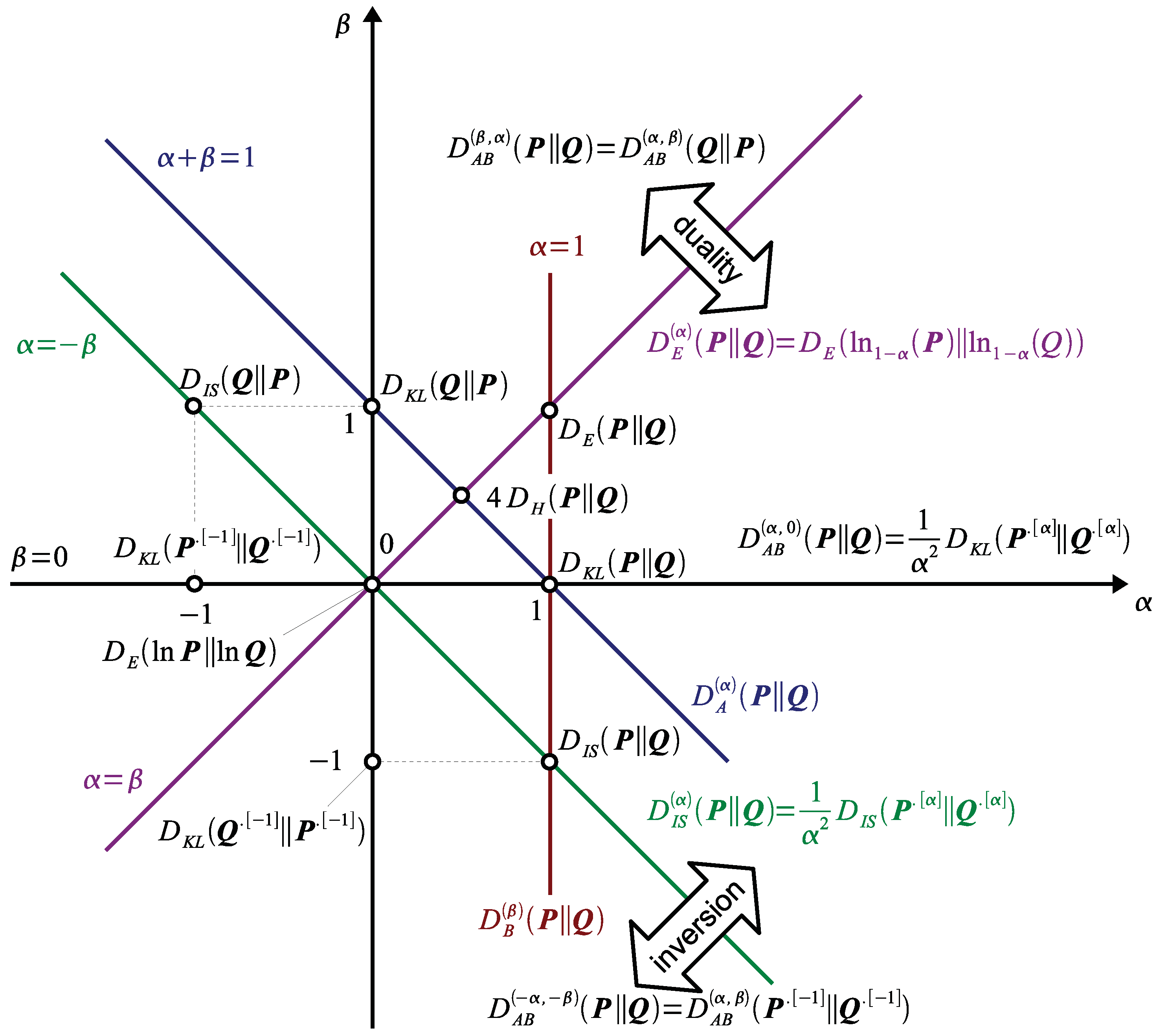
2. The Alpha-Beta Divergences

For positive measures P and Q consider the following new dissimilarity measure, which we shall refer to as the AB-divergence:
D A B ( α , β ) ( P Q ) = 1 α β i t p i t α q i t β α α + β p i t α + β β α + β q i t α + β for α , β , α + β 0 ,
or equivalently
D A B ( α , λ α ) ( P Q ) = 1 ( α λ ) α i t p i t α q i t λ α α λ p i t λ λ α λ q i t λ , for α 0 , α λ , λ = α + β 0 ,
Note that, Equation (19) is a divergence since the following relationship holds:
1 α β p i t α q i t β 1 β ( α + β ) p i t α + β + 1 α ( α + β ) q i t α + β , for α , β , α + β 0 ,
with equality holding for p i t = q i t . In Appendix A, we show that Equation (21) is a summarization of three different inequalities of Young’s type, each one holding true for a different combination of the signs of the constants: α β , α ( α + β ) and β ( α + β ) .
In order to avoid indeterminacy or singularity for certain values of parameters, the AB-divergence can be extended by continuity (by applying l’Hôpital formula) to cover all the values of α , β R , thus the AB-divergence can be expressed or defined in a more explicit form:
D A B ( α , β ) ( P Q ) = i t d A B ( α , β ) ( p i t , q i t ) ,
where
d A B ( α , β ) ( p i t , q i t ) = l l 1 α β p i t α q i t β α ( α + β ) p i t α + β β ( α + β ) q i t α + β for α , β , α + β 0 1 α 2 p i t α ln p i t α q i t α p i t α + q i t α for α 0 , β = 0 1 α 2 ln q i t α p i t α + q i t α p i t α 1 1 for α = β 0 1 β 2 q i t β ln q i t β p i t β q i t β + p i t β for α = 0 , β 0 1 2 ln p i t ln q i t 2 for α , β = 0 .

2.1. Special Cases of the AB-Divergence

We shall now illustrate that a suitable choice of the ( α , β ) parameters simplifies the AB-divergence into some existing divergences, including the well-known Alpha- and Beta-divergences [4,7,19,35].
When α + β = 1 the AB-divergence reduces to the Alpha-divergence [4,33,34,35,52]
D A B ( α , 1 α ) P Q = D A ( α ) P Q
1 α ( α 1 ) i t p i t α q i t 1 α α p i t + ( α 1 ) q i t for α 0 , α 1 , i t p i t ln p i t q i t p i t + q i t for α = 1 , i t q i t ln q i t p i t q i t + p i t for α = 0 .
On the other hand, when α = 1 , it reduces to the Beta-divergence [8,9,19,32,53]
D A B ( 1 , β ) P Q = D B ( β ) ( P Q )
1 β i t p i t q i t β 1 ( 1 + β ) p i t 1 + β β ( 1 + β ) q i t 1 + β for β , 1 + β 0 , 1 2 i t p i t q i t 2 for β = 1 , i t p i t ln p i t q i t p i t + q i t for β = 0 , i t ln q i t p i t + q i t p i t 1 1 for β = 1 .
The AB-divergence gives to the standard Kullback-Leibler (KL) divergence ( D K L ( · , · ) ) for α = 1 and β = 0
D A B ( 1 , 0 ) ( P Q ) = D K L P Q = i t p i t ln p i t q i t p i t + q i t ,
and reduces to the standard Itakura-Saito divergence ( D I S ( · , · ) ) for α = 1 and β = 1 [8,53,54]
D A B ( 1 , 1 ) ( P Q ) = D I S P Q = i t ln q i t p i t + p i t q i t 1 .
Using the 1 α deformed logarithm defined as
ln 1 α ( z ) = z α 1 α , α 0 , ln z , α = 0 ,
where z > 0 , observe that the AB-divergence is symmetric with respect to both arguments for α = β 0 and takes the form of a metric distance
D A B ( α , α ) ( P Q ) = D E ( ln 1 α ( P ) ln 1 α ( Q ) ) = 1 2 i t ln 1 α ( p i t ) ln 1 α ( q i t ) 2 ,
in the transform domain ϕ ( x ) = ln 1 α ( x ) . As particular cases, this includes the scaled squared Euclidean distance (for α = 1 ) and the Hellinger distance (for α = 0 . 5 ).
For both α 0 and β 0 , the AB-divergence converges to the Log-Euclidean distance defined as
D A B ( 0 , 0 ) ( P Q ) = lim α 0 D A B ( α , α ) ( P Q ) = 1 2 i t ln p i t ln q i t 2 .

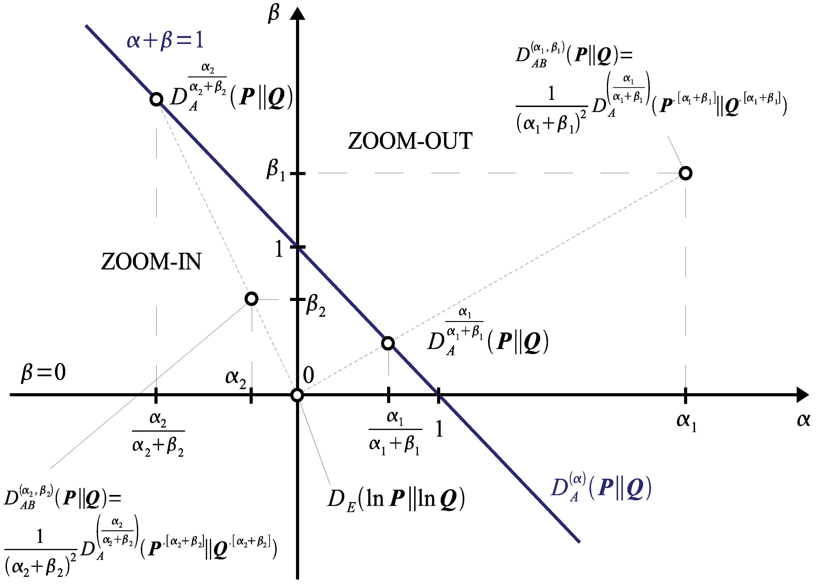
2.2. Properties of AB-Divergence: Duality, Inversion and Scaling

Let us denote by P . [ r ] the one to one transformation that raises each positive element of the matrix P to the power r, i.e., each entry is raised to power r, that is p i t r . According to the definition of the AB-divergence, we can easily check that it satisfies the following duality property (see Figure 1)
D A B ( α , β ) ( P Q ) = D A B ( β , α ) ( Q P ) ,
and inversion property
D A B ( α , β ) ( P Q ) = D A B ( α , β ) ( P . [ 1 ] ) Q . [ 1 ] ) .
The above properties can be considered as a particular case of the scaling property of parameters α and β by a common factor ω R \ { 0 } . The divergence whose parameters has been rescaled is proportional to original divergence with both arguments raised to the common factor, i.e.,
D A B ( ω α , ω β ) ( P Q ) = 1 ω 2 D A B ( α , β ) ( P . [ ω ] Q . [ ω ] ) .
The scaling of α and β by a common factor ω < 1 can be seen as a ‘zoom-in’ on the arguments P and Q . This zoom gives more relevance to the smaller values over the large values. On the other hand, for ω > 1 yields a ‘zoom-out’ effect were the smaller values decrease their relevance at the expense of large values whose relevance is increased (see Figure 1).
Figure 1. Graphical illustration of duality and inversion properties of the AB-divergence. On the alpha-beta plane are indicated as special important cases particular divergences by points and lines, especially Kullback-Leibler divergence D K L , Hellinger Distance D H , Euclidean distance D E , Itakura-Saito distance D I S , Alpha-divergence D A ( α ) , and Beta-divergence D B ( β ) .
Entropy 13 00134 g001
By scaling arguments of the AB-divergence by a positive scaling factor c > 0 , it yields the following relation
D A B ( α , β ) ( c P c Q ) = c α + β D A B ( α , β ) ( P Q ) .
These basic properties imply that whenever α 0 , we can rewrite the AB-divergence in terms of a β α -order Beta-divergence combined with an α-zoom of its arguments as
D A B ( α , β ) ( P Q ) = 1 α 2 D A B 1 , β α ( P . [ α ] Q . [ α ] )
= 1 α 2 D B β α ( P . [ α ] Q . [ α ] ) .
Similarly, for α + β 0 , the AB-divergence can also be expressed in terms of α α + β -order Alpha-divergence with an ( α + β ) -zoom of the arguments (see Figure 2) as
D A B ( α , β ) ( P Q ) = 1 ( α + β ) 2 D A B α α + β , β α + β ( P . [ α + β ] Q . [ α + β ] )
= 1 ( α + β ) 2 D A ( α α + β ) P . [ α + β ] Q . [ α + β ] .
illustrating that the AB-divergence equals to an α α + β -order Alpha-divergence with an ( α + β ) -zoom in of the arguments. On the other hand D A B ( α 1 , β 1 ) can be seen as an Alpha-divergence of order α 1 / ( α 1 + β 1 ) of a zoom-out of the arguments (with α 1 + β 1 > 1 ). Note that, D A B ( α 2 , β 2 ) can be seen as the Alpha-divergence of order α 2 / ( α 2 + β 2 ) with a zoom-in of its arguments with α 2 + β 2 < 1 (see Figure 2).
Figure 2. Illustrations how the AB-divergence for α + β 0 can be expressed via scaled Alpha-divergences.
Entropy 13 00134 g002
When α 0 and β = 0 , the AB-divergence can be expressed in terms of the Kullback-Leibler divergence with an α-zoom of its arguments
D A B ( α , 0 ) ( P Q ) = 1 α 2 D A B ( 1 , 0 ) P . [ α ] Q . [ α ]
= 1 α 2 D K L P . [ α ] Q . [ α ]
= 1 α 2 i t p i t α ln p i t α q i t α p i t α + q i t α .
When α + β = 0 with α 0 and β 0 , the AB-divergence can also be expressed in terms of a generalized Itakura-Saito distance with an α-zoom of the arguments
D A B ( α , α ) ( P Q ) = 1 α 2 D A B 1 , 1 ( P . [ α ] Q . [ α ] )
= 1 α 2 D I S P . [ α ] Q . [ α ]
= 1 α 2 i t ln q i t α p i t α + p i t α q i t α 1 .
Remark: 
The generalized Itakura-Saito distance is scale-invariant, i.e,
D A B ( α , α ) ( P Q ) = D A B ( α , α ) ( c P c Q ) ,
with any c > 0 .
Note that, from the AB-divergence, a more general scale-invariant divergence can be obtained by the monotonic nonlinear transformations:
i t p i t α q i t β ln i t p i t α q i t β α , β
leading to the following scale-invariant divergence given by
D A C ( α , β ) ( P Q ) = 1 β ( α + β ) ln i t p i t α + β + 1 α ( α + β ) ln i t q i t α + β 1 α β ln i t p i t α q i t β = 1 α β ln i t p i t α + β α α + β i t q i t α + β β α + β i t p i t α q i t β for α 0 , β 0 , α + β 0 .
which generalizes a family of Gamma-divergences [35].
The divergence (49) is scale-invariant in a more general context
D A C ( α , β ) ( P | | Q ) = D A C ( α , β ) ( c 1 P | | c 2 Q )
for any positive scale factors c 1 and c 2 .

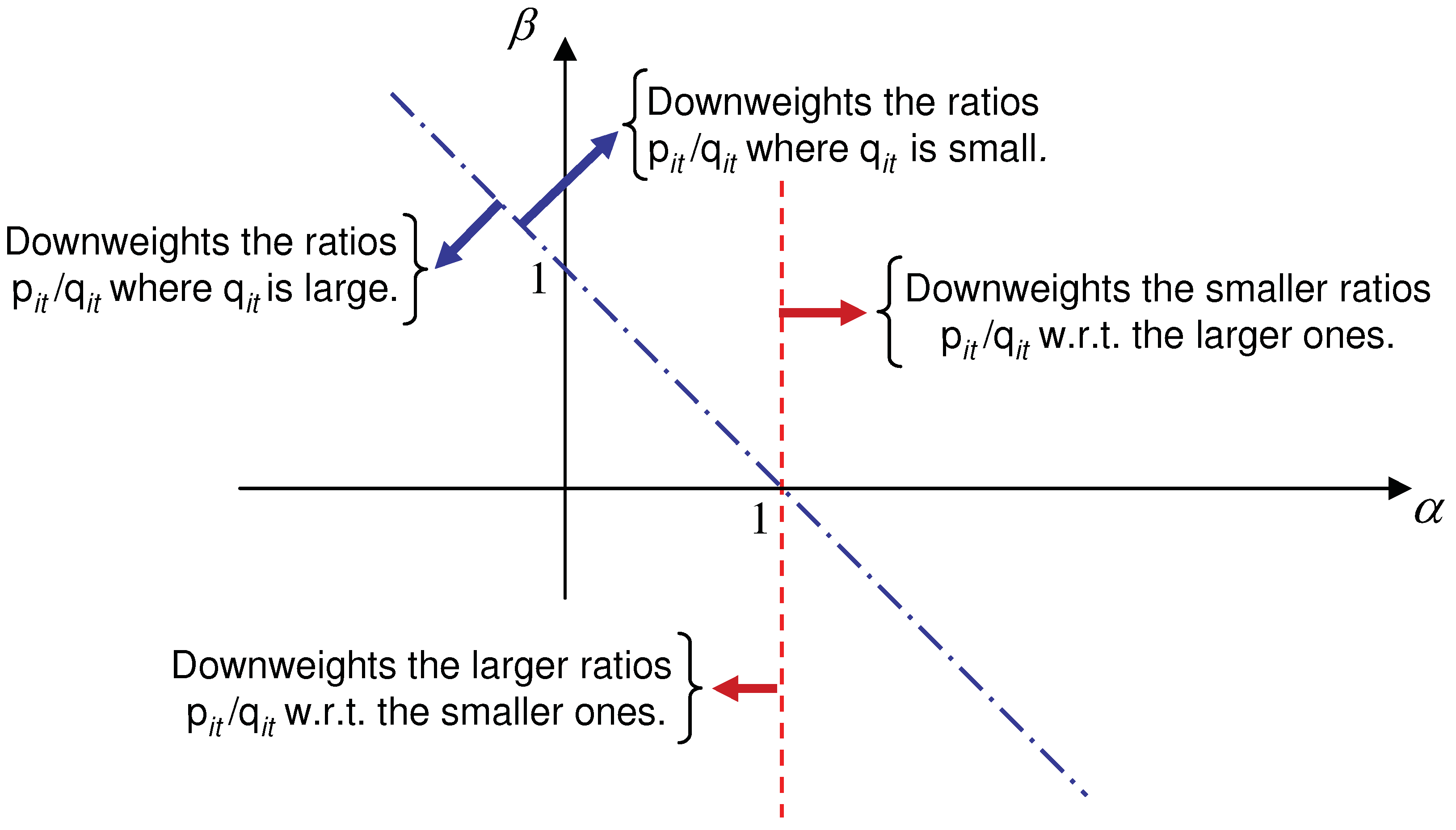
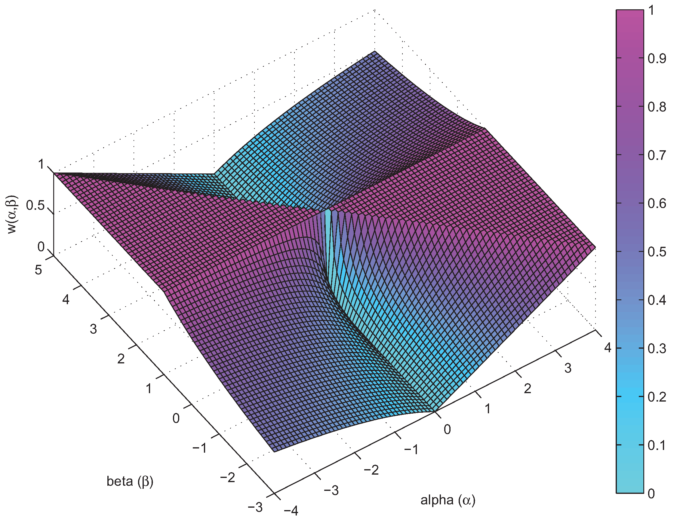
2.3. Why is AB-Divergence Potentially Robust?

To illustrate the role of the hyperparameters α and β on the robustness of the AB-divergence with respect to errors and noises, we shall compare the behavior of the AB-divergence with the standard Kullback-Leibler divergence. We shall assume, without loss of generality, that the proposed factorization model Q (for given noisy P ) is a function of the vector of parameters θ and that each of its elements q i t ( θ ) > 0 is non-negative for a certain range of parameters Θ.
The estimator θ ^ obtained for the Kullback-Leibler divergence between two discrete positive measures P and Q , is a solution of
D K L P Q θ = i t q i t θ ln 0 p i t q i t = 0 ,
while, for the Beta-divergence, the estimator solves
D B ( β ) P Q θ = i t q i t θ q i t β ln 0 p i t q i t = 0 .
The main difference between both equations is in the weighting factors q i t β for the Beta-divergence which are controlled by the parameter β. In the context of probability distributions, these weighting factors may control the influence of likelihood ratios p i t / q i t . It has been shown [55] and [56] that the parameter β determines a tradeoff between robustness to outliers (for β > 0 ) and efficiency (for β near 0). In the special case of β = 1 the Euclidean distance is obtained, which is known to be more robust and less efficient than the Kullback-Leibler divergence β = 0 .
On the other hand, for the Alpha-divergence, the estimating equation takes a different form
D A ( α ) P Q θ = i t q i t θ ln 1 α p i t q i t = 0 .
In this case, the influence of the values of individual ratios p i t / q i t are controlled not by weighting factors but by the deformed logarithm of order 1 α . This feature can be interpreted as a zoom or over-weight of the interesting details of the likelihood ratio. For α > 1 (a zoom-out), we emphasize the relative importance of larger values of the ratio p i t / q i t , whereas for α < 1 (a zoom-in), we put more emphasis on smaller values of p i t / q i t (see Figure 3). The major consequence is the inclusive ( α ) and exclusive ( α ) behavior of the Alpha-divergence discussed in [52].
The estimating equation for the Alpha-Beta divergence combines both effects:
D A B ( α , β ) P Q θ = i t q i t θ q i t α + β 1 w e i g h t s ln 1 α p i t / q i t α z o o m = 0 ,
and therefore is much more flexible and powerful regarding insensitivity to error and noise.
As illustrated in Figure 3, depending on value of α, we can zoom-in or zoom-out the interesting sets of the ratios p i t / q i t and simultaneously weight these ratios by scaling factors q i t λ 1 controlled by the parameter λ = α + β . Therefore, the parameter α can be used to control the influence of large or small ratios in the estimator, while the parameter β provides some control on the weighting of the ratios depending on the demand to better fit to larger or smaller values of the model.
Figure 3. Graphical illustration how the set parameters ( α , β ) can control influence of individual ratios p i t / q i t . The dash-doted line ( α + β = 1 ) shows the region where the multiplicative weighting factor q i t α + β 1 in the estimating equations is constant and equal to unity. The dashed line ( α = 1 ) shows the region where the order of the deformed logarithm of p i t / q i t is constant and equal to that of the standard Kullback-Leibler divergence.
Entropy 13 00134 g003

3. Generalized Multiplicative Algorithms for NMF

3.1. Derivation of Multiplicative NMF Algorithms Based on the AB-Divergence

We shall now develop generalized and flexible NMF algorithms (see Equation (1)) by employing the AB-divergence with Y = P = [ p i t ] R + I × T , Q = [ q i t ] = A X R + I × T , where q i t = p ^ i t = [ A X ] i t = j a i j x j t . In this case, the gradient of the AB-divergence (20) can be expressed in a compact form (for any α , β R ) in terms of an 1 α deformed logarithm (see (30))
D A B ( α , β ) x j t = i = 1 I q i t λ 1 a i j ln 1 α p i t q i t ,
D A B ( α , β ) a i j = t = 1 T q i t λ 1 x j t ln 1 α p i t q i t .
The new multiplicative learning algorithm is gradient descent based, in the natural parameter space ϕ ( x ) of the proposed divergence:
x j t ϕ 1 ϕ ( x j t ) η j t D A B ( α , β ) ϕ ( x j t ) ,
a i j ϕ 1 ϕ ( a i j ) η i j D A B ( α , β ) ϕ ( a i j ) .
These updates can be considered as a generalization of the exponentiated gradient (EG) [57].
In general, such a nonlinear scaling (or transformation) provides a stable solution and the obtained gradients are much better behaved in the ϕ space. We use the 1 α deformed logarithm transformation ϕ ( z ) = ln 1 α ( z ) , whose inverse transformation is a 1 α deformed exponential
ϕ 1 ( z ) = exp 1 α ( z ) = exp ( z ) for α = 0 , ( 1 + α z ) 1 α for α 0 and 1 + α z 0 , 0 for α 0 and 1 + α z < 0 .
For positive measures z > 0 , the direct transformation ϕ ( z ) and the composition ϕ 1 ( ϕ ( z ) ) are bijective functions which define a one to one correspondence, so we have ϕ 1 ( ϕ ( z ) ) = z .
By choosing suitable learning rates
η j t = x j t 2 α 1 i = 1 I a i j q i t λ 1 , η i j = a i j 2 α 1 t = 1 T x j t q i t λ 1 .
a new multiplicative NMF algorithm (refereed to as the AB-multiplicative NMF algorithm) is obtained as:
x j t x j t exp 1 α i = 1 I a i j q i t λ 1 i = 1 I a i j q i t λ 1 ln 1 α p i t q i t , a i j a i j exp 1 α t = 1 T x j t q i t λ 1 t = 1 t x j t q i t λ 1 ln 1 α p i t q i t .
In these equations, the deformed logarithm of order 1 α of the quotients p i t / q i t plays a key role to control relative error terms whose weighted mean provides the multiplicative corrections. This deformation in the relative error is controlled by the parameter α. The parameter α > 1 gives more relevance to the large values of the quotient, while the case of α < 1 puts more emphasis on smaller values of the quotient. On the other hand, the parameter λ 1 (where λ = α + β ) controls the influence of the values of the approximation ( q i t ) on the weighing of the deformed error terms. For λ = 1 , this influence disappears.
It is interesting to note that the multiplicative term of the main updates
M α ( z , w , S ) = exp 1 α 1 i S w i i S w i ln 1 α z i ,
can be interpreted as a weighted generalized mean across the elements with indices in the set S.
Depending on the value of α, we obtain as particular cases: the minimum of the vector z (for α ), its weighted harmonic mean ( α = 1 ), the weighted geometric mean ( α = 0 ), the arithmetic mean ( α = 1 ), the weighted quadratic mean ( α = 2 ) and the maximum of the vector ( α ), i.e.,
M α ( z , w , { 1 , , n } ) = min { z 1 , , z n } , α , i = 1 n w i i = 1 n w i z i 1 , α = 1 , i = 1 n z w i i = 1 n w i , α = 0 , 1 i = 1 n w i i = 1 n w i z i , α = 1 , 1 i = 1 n w i i = 1 n w i z i 2 1 / 2 , α = 2 , max { z 1 , , z n } , α .
The generalized weighted means are monotonically increasing functions of α, i.e., if α 1 < α 2 , then
M α 1 ( z , w , S ) < M α 2 ( z , w , S ) .
Thus, by increasing the values of α, we puts more emphasis on large relative errors in the update formulas (61).
In the special case of α 0 , the above update rules can be simplified as:
x j t x j t i = 1 I a i j p i t α q i t β 1 i = 1 I a i j q i t α + β 1 1 / α ,
a i j a i j t = 1 T x j t p i t α q i t β 1 t = 1 T x j t q i t α + β 1 1 / α ,
where q i t = [ A X ] i t and at every iteration the columns of A are normalized to the unit length.
The above multiplicative update rules can be written in a compact matrix forms as
X X A T ( P . [ α ] Q . [ β 1 ] ) A T Q . [ α + β 1 ] . [ 1 / α ] ,
A A P . [ α ] Q . [ β 1 ] X T Q . [ α + β 1 ] X T . [ 1 / α ]
or even more compactly:
X X A T Z A T Q . [ α + β 1 ] . [ 1 / α ] ,
A A Z X T Q . [ α + β 1 ] X T . [ 1 / α ] ,
where Z = P . [ α ] Q . [ β 1 ] .
In order to fix the scaling indeterminacy between the columns of A and the rows of X , in practice, after each iteration, we can usually evaluate the l 1 -norm of the columns of A and normalize the elements of the matrices as
x i j x i j p a p j , a i j a i j / p a p j .
This normalization does not alter Q = A X , thus, preserving the value of the AB-divergence.
The above novel algorithms are natural extensions of many existing algorithms for NMF, including the ISRA, EMML, Lee-Seung algorithms and Alpha- and Beta-multiplicative NMF algorithms [7,58]. For example, by selecting α + β = 1 , we obtain the Alpha-NMF algorithm, for α = 1 , we have Beta-NMF algorithms, for α = β 0 we obtain a family of multiplicative NMF algorithms based on the extended Itakura-Saito distance [8,53]. Furthermore, for α = 1 and β = 1 , we obtain the ISRA algorithm and for α = 1 and β = 0 we obtain the EMML algorithm.
It is important to note that in low-rank approximations, we do not need access to all input data p i t . In other words, the above algorithms can be applied for low-rank approximations even if some data are missing or they are purposely omitted or ignored. For large-scale problems, the learning rules can be written in a more efficient form by restricting the generalized mean only to those elements whose indices belong to a preselected subsets S T { 1 , , T } and S I { 1 , , I } of the whole set of indices.
Using a duality property ( D A B ( α , β ) ( P Q ) = D A B ( β , α ) ( Q P ) ) of the AB-divergence, we obtain now the dual update rules:
x j t x j t exp 1 β i S I a i j p i t λ 1 i S I a i j p i t λ 1 ln 1 β q i t p i t , a i j a i j exp 1 β t S T x j t p i t λ 1 t S T x j t p i t λ 1 ln 1 β q i t p i t ,
which for β 0 reduce to
a i j a i j t S T x j t p i t α 1 q i t β t S T x j t p i t α + β 1 1 / β , x j t x j t i S I a i j p i t α 1 q i t β i S I a i j p i t α + β 1 1 / β .

3.2. Conditions for a Monotonic Descent of AB-Divergence

In this section, we first explain the basic principle of auxiliary function method, which allows us to establish conditions for which NMF update rules provide monotonic descent of the cost function during iterative process. In other words, we analyze the conditions for the existence of auxiliary functions that justify the monotonous descent in the AB-divergence under multiplicative update rules of the form (61). NMF update formulas with such property have been previously obtained for certain particular divergences: in [38,41] for the Euclidean distance and Kullback-Leibler divergence, in [58] for the Alpha-Divergence and in [59,60,61] for the Beta-divergence.
Let Q ( k ) = A ( k ) X ( k ) denote our current factorization model of the observations in the k-th iteration, and let { Q ( k + 1 ) } denote our candidate model for the next k + 1 -iteration. In the following, we adopt the notation { Q ( k ) } { A ( k ) , X ( k ) } to refer compactly to the non-negative factors of the decompositions.
An auxiliary function G ( { Q ( k + 1 ) } , { Q ( k ) } ; P ) for the surrogate optimization of the divergence should satisfy
G ( { Q ( k + 1 ) } , { Q ( k ) } ; P ) G ( { Q ( k + 1 ) } , { Q ( k + 1 ) } ; P ) = D A B ( α , β ) ( P | | Q ( k + 1 ) ) ,
with equality holding for { Q ( k ) } = { Q ( k + 1 ) } .
In analogy to the Expectation Maximization techniques developed in [38,41,58], our objective is to find a convex upper bound of the AB divergence and to replace the minimization of the original AB-divergence by an iterative optimization of the auxiliary function.
Given the factors of the current factorization model { Q ( k ) } , the factors of the next candidate { Q ( k + 1 ) } are chosen as
{ Q ( k + 1 ) } = arg min { Q } G ( { Q } , { Q ( k ) } ; P ) .
where, for simplicity, the minimization is usually carried out with respect to only one of the factors A or X of { Q } , while keeping the other factor fixed and common in { Q ( k + 1 ) } , { Q ( k ) } and { Q } .
Assuming that auxiliary function is found, a monotonic descent of the AB-divergence is a consequence of the chain of inequalities:
D A B ( α , β ) ( P | | Q ( k ) ) = G ( { Q ( k ) } , { Q ( k ) } ; P )
( a ) G ( { Q ( k + 1 ) } , { Q ( k ) } ; P )
( b ) G ( { Q ( k + 1 ) } , { Q ( k + 1 ) } ; P )
= D A B ( α , β ) ( P Q ( k + 1 ) ) .
The inequality ( a ) is due to the optimization in (75), while the inequality ( b ) reflects the definition of the auxiliary function in (74).

3.3. A Conditional Auxiliary Function

It is shown in Appendix B that under a certain condition, the function
G ( { Q ( k + 1 ) } , { Q ( k ) } ; P ) = i , t j γ i t ( j ) ( { Q ( k ) } ) d A B ( α , β ) p i t , q ^ i t ( j )
where γ i t ( j ) ( { Q ( k ) } ) = a i j ( k ) x j t ( k ) q i t ( k ) and q ^ i t ( j ) = a i j ( k + 1 ) x j t ( k + 1 ) γ i t ( j ) ( { Q ( k ) } ) ,
is an auxiliary function for the surrogate optimization of D A B ( α , β ) ( P | | Q ) . The required condition is, at each iteration, the convexity of d A B ( α , β ) ( p i t , q ^ i t ) with respect to all q ^ i t [ min j q ^ i t ( j ) , max j q ^ i t ( j ) ] .
Recall that Q ( k ) = A ( k ) X ( k ) corresponds to the current iteration, while a candidate model Q ( k + 1 ) = A ( k + 1 ) X ( k + 1 ) for the next iteration, is the solution of the optimization problem (75). For updating A at each iteration, we keep X ( k + 1 ) equal to X ( k ) and find the global minimum of the auxiliary function G ( { A ( k + 1 ) , X ( k ) } , { A ( k ) , X ( k ) } ; P ) with respect to A ( k + 1 ) .
By setting the following derivative to zero
G ( A X , Q ( k ) ; P ) a i j = a i j β 1 t = 1 T ( q i t ( k ) ) λ 1 x j t ( k ) ln 1 α a i j a i j ( k ) ln 1 α p i t q i t ( k ) = 0 ,
and solving with respect to a i j = a i j ( k + 1 ) yields
a i j ( k + 1 ) = a i j ( k ) exp 1 α t = 1 T ( q i t ( k ) ) λ 1 x j t ( k ) t = 1 T ( q i t ( k ) ) λ 1 x j t ( k ) ln 1 α p i t q i t ( k ) .
Analogously, for the intermediate factorized model Q ˜ ( k ) = A ( k + 1 ) X ( k ) , the global minimum of the auxiliary function G ( A ( k + 1 ) X ( k + 1 ) , { A ( k + 1 ) , X ( k ) } ; P ) with respect to the new update X ( k + 1 ) , while keeping A = A ( k + 1 ) , is given by
x j t ( k + 1 ) = x j t ( k ) exp 1 α i = 1 I ( q ˜ i t ( k ) ) λ 1 a i j ( k + 1 ) i = 1 I ( q ˜ i t ( k ) ) λ 1 a i j ( k + 1 ) ln 1 α p i t q ˜ i t ( k ) .
The above two equations match with the updates proposed in (61). As previously indicated, a sufficient condition for a monotonic descent of the AB-divergence is the convexity of terms d A B ( α , β ) ( p i t , q ^ i t ) for all q ^ i t [ min j q ^ i t ( j ) , max j q ^ i t ( j ) ] . At this point, it is illustrative to interpret the elements q ^ i t ( j ) defined in (81) as linear predictions the factorization model q i t = j a i j x j t , obtained from the components a i j x j t and factors γ i t ( j ) ( { Q ( k ) } ) .
Appendix C, provides necessary and sufficient conditions for the convexity of d A B ( α , β ) ( p i t , q ^ i t ) with respect to q ^ i t . Depending on the parameter β, it is required that one of the following condition be satisfied:
p i t q ^ i t c ( α , β ) for β < min { 1 , 1 α } , always convex for β [ min { 1 , 1 α } , max { 1 , 1 α } ] , p i t q ^ i t c ( α , β ) for β > max { 1 , 1 α } ,
where the upper and lower bounds depend on the function
c ( α , β ) = exp 1 α 1 β 1 ,
whose contour plot is shown in Figure 4(b).
The convexity of the divergence w.r.t. q i t holds for the parameters ( α , β ) within the convex cone of β [ min { 1 , 1 α } , max { 1 , 1 α } ] . Therefore, for this set of parameters, the monotonic descent in the AB-divergence with the update formulas (83), (84) is guaranteed.
Figure 4. Convexity analysis of d A B ( α , β ) ( p i t , q ^ i t ) w.r.t. q ^ i t in the ( α , β ) plane.
Entropy 13 00134 g004
On the other hand, even when β [ min { 1 , 1 α } , max { 1 , 1 α } ] , we can still guarantee the monotonic descent if the set of estimators q ^ i t [ min j q ^ i t ( j ) , max j q ^ i t ( j ) ] is bounded and sufficiently close to p i t so that they satisfy the conditions (85). Figure 4(b) illustrates this property demonstrating that if the ratios p i t q ^ i t approach unity, the convexity of the divergence w.r.t. q i t holds for an increasing size of ( α , β ) plane. In other words, for sufficiently small relative errors between p i t and q ^ i t , the update formulas (83), (84) still guarantee a monotonic descent of the AB-divergence, within a reasonable wide range of the hyperparameters ( α , β ) .

3.4. Unconditional Auxiliary Function

The conditions of the previous section for a monotonic descent can be avoided by upper-bounding d A B ( α , β ) p i t , q ^ i t with another function d ¯ A B ( α , β ) p i t , q ^ i t ; q i t ( k ) which is convex with respect to q ^ i t and, at the same time, tangent to the former curve at q ^ i t = q i t ( k ) , i.e.,
d A B ( α , β ) p i t , q i t d ¯ A B ( α , β ) p i t , q ^ i t ; q i t ( k ) ,
where
d A B ( α , β ) p i t , q i t ( k ) = d ¯ A B ( α , β ) p i t , q i t ( k ) , q i t ( k ) ,
and
2 d ¯ A B ( α , β ) p i t , q ^ i t ; q i t ( k ) q ^ i t 2 0 .
Similarly to the approach in [59,60,61] for the Beta-divergence, we have constructed an auxiliary function for the AB-divergence by linearizing those additive concave terms of the AB-divergence:
d ¯ A B ( α , β ) p i t , q ^ i t ; q i t ( k ) = p i t α + β β ( α + β ) + ( q i t ( k ) ) α + β α ( α + β ) p i t α q ^ i t β α β + ( q i t ( k ) ) α + β 1 α ( q ^ i t q i t ( k ) ) , β α < 1 α 1 , p i t α + β β ( α + β ) + q ^ i t α + β α ( α + β ) p i t α q ^ i t β α β , β α [ 1 α 1 , 1 α ] , p i t α + β β ( α + β ) + q ^ i t α + β α ( α + β ) p i t α ( q i t ( k ) ) β α β p i t α ( q i t ( k ) ) β 1 α ( q ^ i t q i t ( k ) ) , β α > 1 α .
The upper-bounds for singular cases can be obtained by continuity using L’Hópitals formula.
The unconditional auxiliary function for the surrogate minimization of the AB-divergence D A B ( α , β ) ( P | | Q ) is now given by
G ¯ ( { Q } , { Q ( k ) } ; P ) = i , t j γ i t ( j ) ( { Q ( k ) } ) d ¯ A B ( α , β ) p i t , q ^ i t ( j ) ; q i t ( k ) ,
where γ i t ( j ) ( { Q ( k ) } ) = a i j ( k ) x j t ( k ) q i t ( k ) and q ^ i t ( j ) = a i j ( k + 1 ) x j t ( k + 1 ) γ i t ( j ) ( { Q ( k ) } ) .
The alternating minimization of the above auxiliary function with respect to A and X yields the following stabilized iterations (with monotonic descent of the AB-divergence):
a i j ( k + 1 ) = a i j ( k ) exp 1 α t = 1 T ( q i t ( k ) ) λ 1 x j t ( k ) t = 1 T ( q i t ( k ) ) λ 1 x j t ( k ) ln 1 α p i t q i t ( k ) w ( α , β ) ,
x j t ( k + 1 ) = x j t ( k ) exp 1 α i = 1 I ( q ˜ i t ( k ) ) λ 1 a i j ( k + 1 ) i = 1 I ( q ˜ i t ( k ) ) λ 1 a i j ( k + 1 ) ln 1 α p i t q ˜ i t ( k ) w ( α , β ) ,
where
w ( α , β ) = 1 α = 0 , β = 1 , 0 α = 0 , β 1 , α 1 β α 0 , β α < 1 α 1 , 1 α 0 , β α [ 1 α 1 , 1 α ] , α α + β 1 α 0 , β α > 1 α .
The stabilized formulas (92), (93) coincide with (83), (84), except for the exponent w ( α , β ) , which is shown in Figure 5. This exponent is bounded between zero and one, and plays a similar role in the multiplicative update to that of the normalized step-size in an additive gradient descent update. Its purpose is to slow down the convergence so as to guarantee monotonic descent of the cost function. This is a consequence of the fact that the multiplicative correction term is progressively contracted towards the unity as w ( α , β ) 0 . For the same reason, the stabilized formulas completely stop the updates for α = 0 and β 1 . Therefore, for α close to zero, we recommend to prevent this undesirable situation by enforcing a positive lower-bound in the value of exponent w ( α , β ) .
Figure 5. Surface plot of the exponent w ( α , β ) , whose role in the multiplicative update is similar to that of a normalized step-size in an additive gradient descent update.
Entropy 13 00134 g005

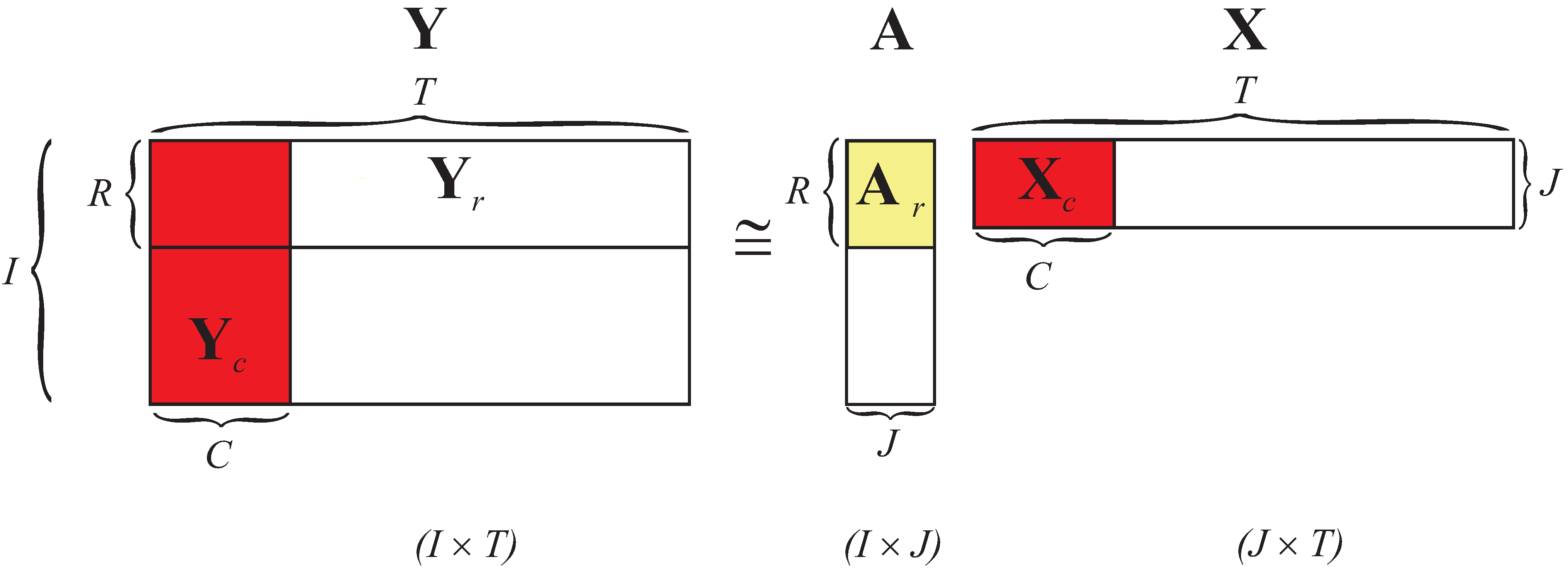
3.5. Multiplicative NMF Algorithms for Large-Scale Low-Rank Approximation

In practice, for low-rank approximations with J min { I , T } we do not need to process or save the whole data matrix Y , nor is it necessary to perform computations at each iteration step of the products of the whole estimated matrices Y T A or Y X T (see Figure 6).
Figure 6. Conceptual factorization model of block-wise data processing for a large-scale NMF. Instead of processing the whole matrix P = Y R + I × T , we can process much smaller block matrices Y c R + I × C and Y r R + R × T and the corresponding factor matrices X c = B c T = [ b 1 , r , b 2 , r , , b J , r ] T R + J × C and A r = [ a 1 , r , a 2 , r , , a J , r ] R + R × J with J < C < < T and J < R < < I . For simplicity of graphical illustration, we have selected the first C columns of the matrices P and X and the first R rows of A .
Entropy 13 00134 g006
In other words, in order to perform the basic low-rank NMF
Y = P = A X + E ,
we need to perform two associated nonnegative matrix factorizations using much smaller-scale matrices for large-scale problems, given by
Y r = A r X + E r , for fixed   ( known ) A r ,
Y c = A X c + E c , for fixed   ( known ) X c ,
where Y r R + R × T and Y c R + I × C are the matrices constructed from the selected rows and columns of the matrix Y , respectively. Analogously, we can construct the reduced matrices: A r R + R × J and X c R + J × C by using the same indices for the columns and rows as those used for the construction of the data sub-matrices Y c and Y r . In practice, it is usually sufficient to choose: J < R 4 J and J < C 4 J .
Using this approach, we can formulate the update learning rule for a large-scale multiplicative NMF as (see Figure 6)
X X A r T ( Y r . [ α ] Q r . [ β 1 ] ) A r T Q r . [ α + β 1 ] . [ w / α ] ,
A A Y c . [ α ] Q c . [ β 1 ] X c T Q c . [ α + β 1 ] X c T . [ w / α ] ,
Q r = A r X , Q c = A X c .
In fact, we need to save only two reduced set of data matrices Y r R + R × T and Y c R + I × C . For example, for large dense data matrix Y R + I × T with I = T = 10 5 and J = 10 and R = C = 50 , we need to save only 10 7 nonzero entries instead of 10 10 entries, thus reducing memory requirement 1000 times.
We can modify and extend AB NMF algorithms in several ways. First of all, we can use for update of matrices A and X two different cost functions, under the assumption that both the functions are convex with respect to one set of updated parameters (another set is assumed to be fixed). In a special case, we can use two AB-divergences (with two different sets of parameters: one D A B ( α A , β A ) ( Y | | A X ) for the estimation of A and fixed X , and another one D A B ( α X , β X ) ( Y | | A X ) for the estimation of X and fixed A ). This leads to the following updates rules
X X A r T ( Y r . [ α X ] Q r . [ β X 1 ] ) A r T Q r . [ α X + β X 1 ] . [ w X / α X ] ,
A A Y c . [ α A ] Q c . [ β A 1 ] X c T Q c . [ α A + β A 1 ] X c T . [ w A / α A ] ,
Q r = A r X , Q c = A X c .
In order to accelerate the convergence of the algorithm, we can estimate one of the factor matrices, e.g., A by using the ALS (Alternating Least Squares) algorithm [7]. This leads to the following modified update rules which can still be robust with respect to X for suitably chosen set of the parameters.
X X A r T ( Y r . [ α ] ( A r X ) . [ β 1 ] ) A r T ( A r X ) . [ α + β 1 ] . [ w / α ] ,
A max { Y r X r T ( X r X r T ) 1 , ε } .
Another alternative exists, which allows us to use different cost functions and algorithms for each of the factor matrices.
Furthermore, it would be very interesting to apply AB-multiplicative NMF algorithms for inverse problems in which matrix A is known and we need to estimate only matrix X for ill-conditioned and noisy data [62,63].

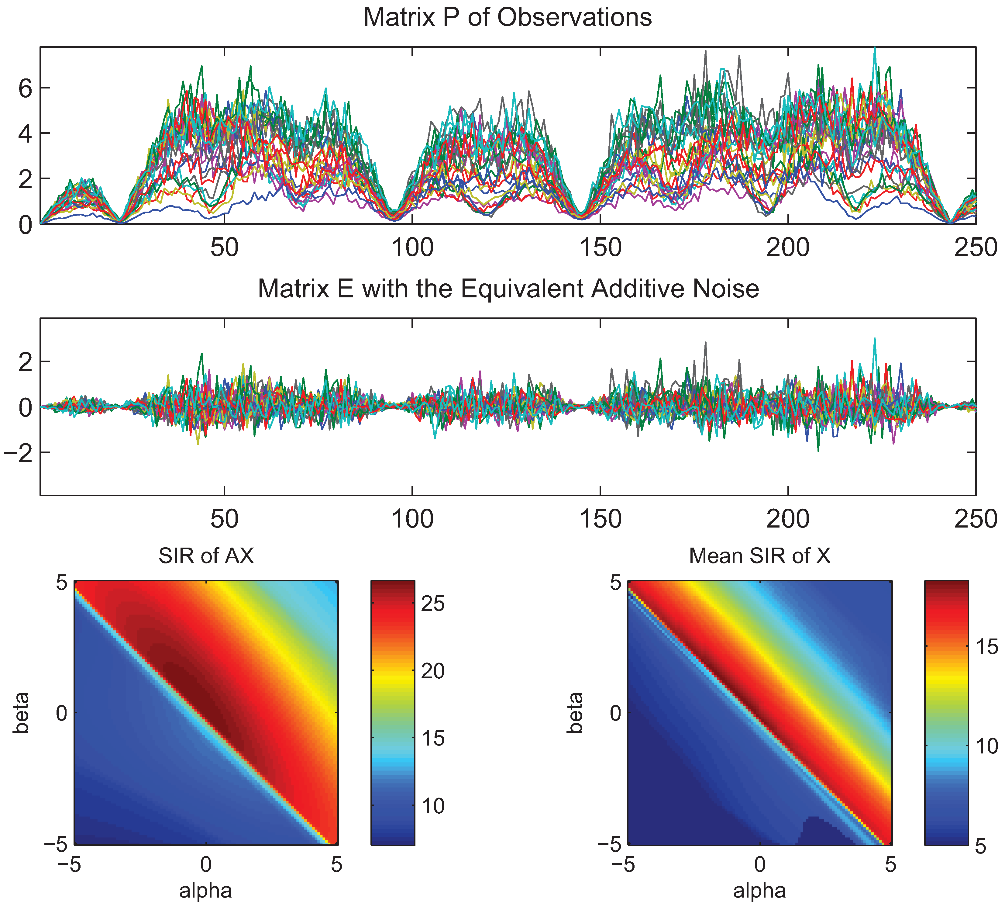
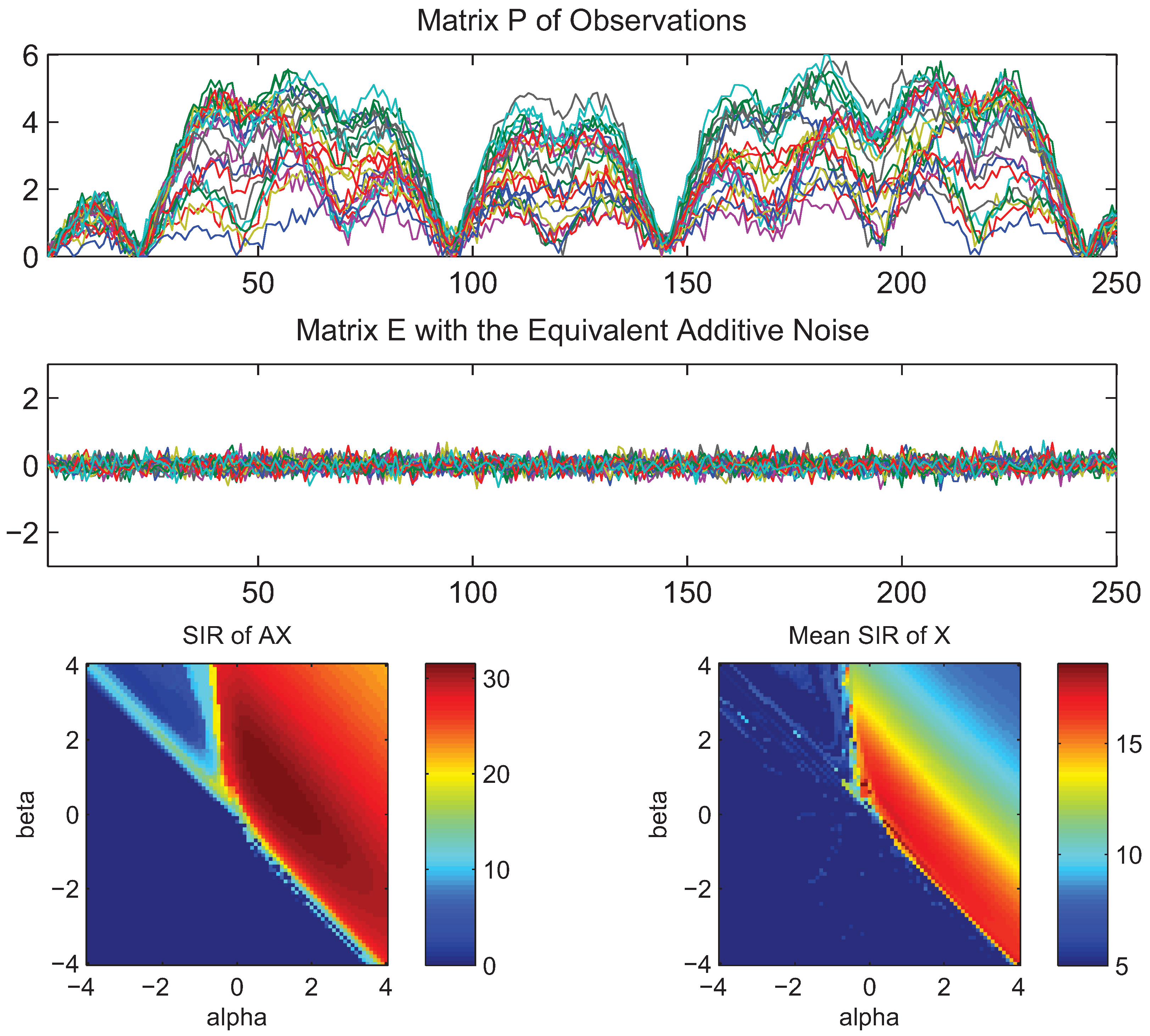
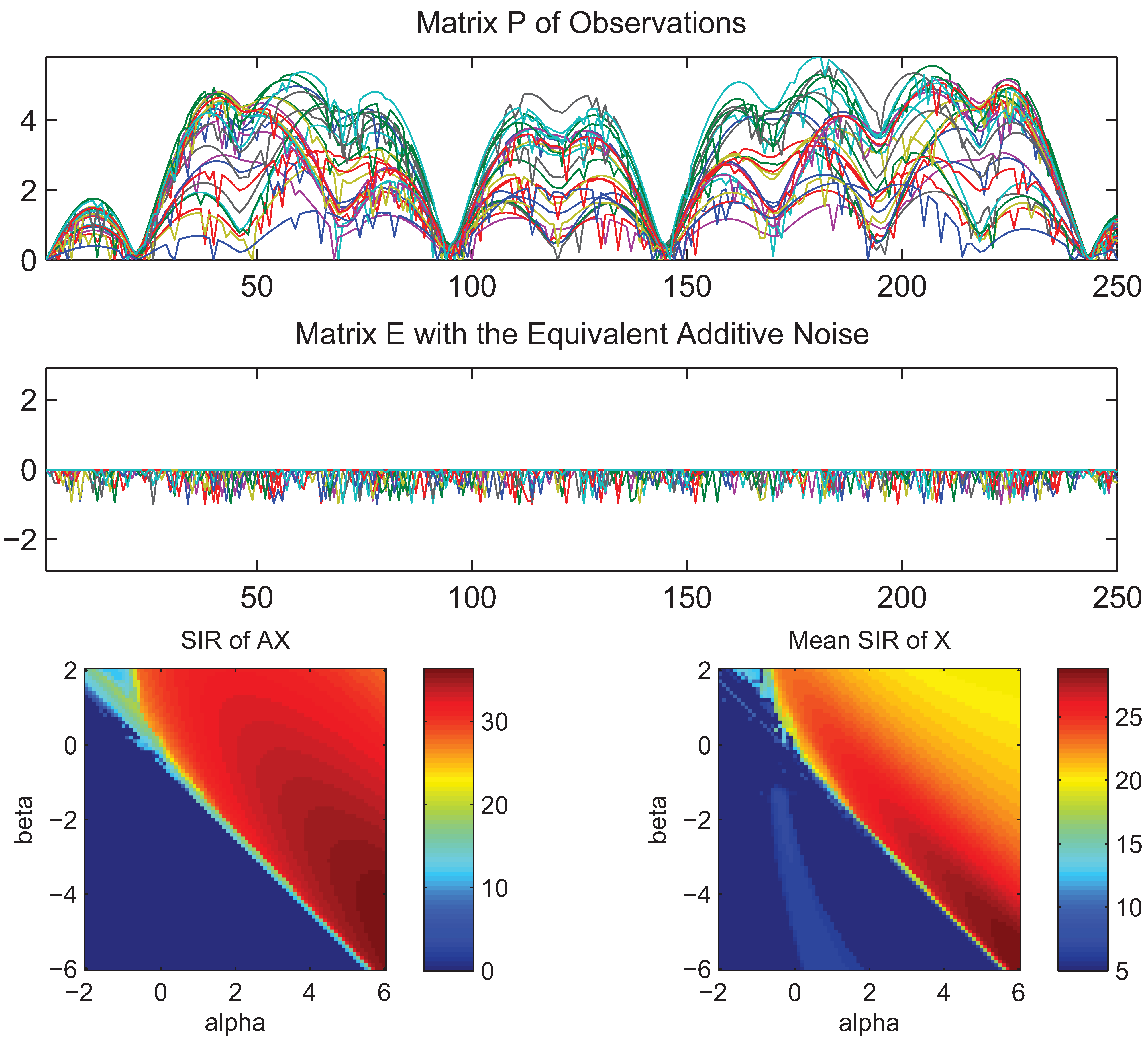
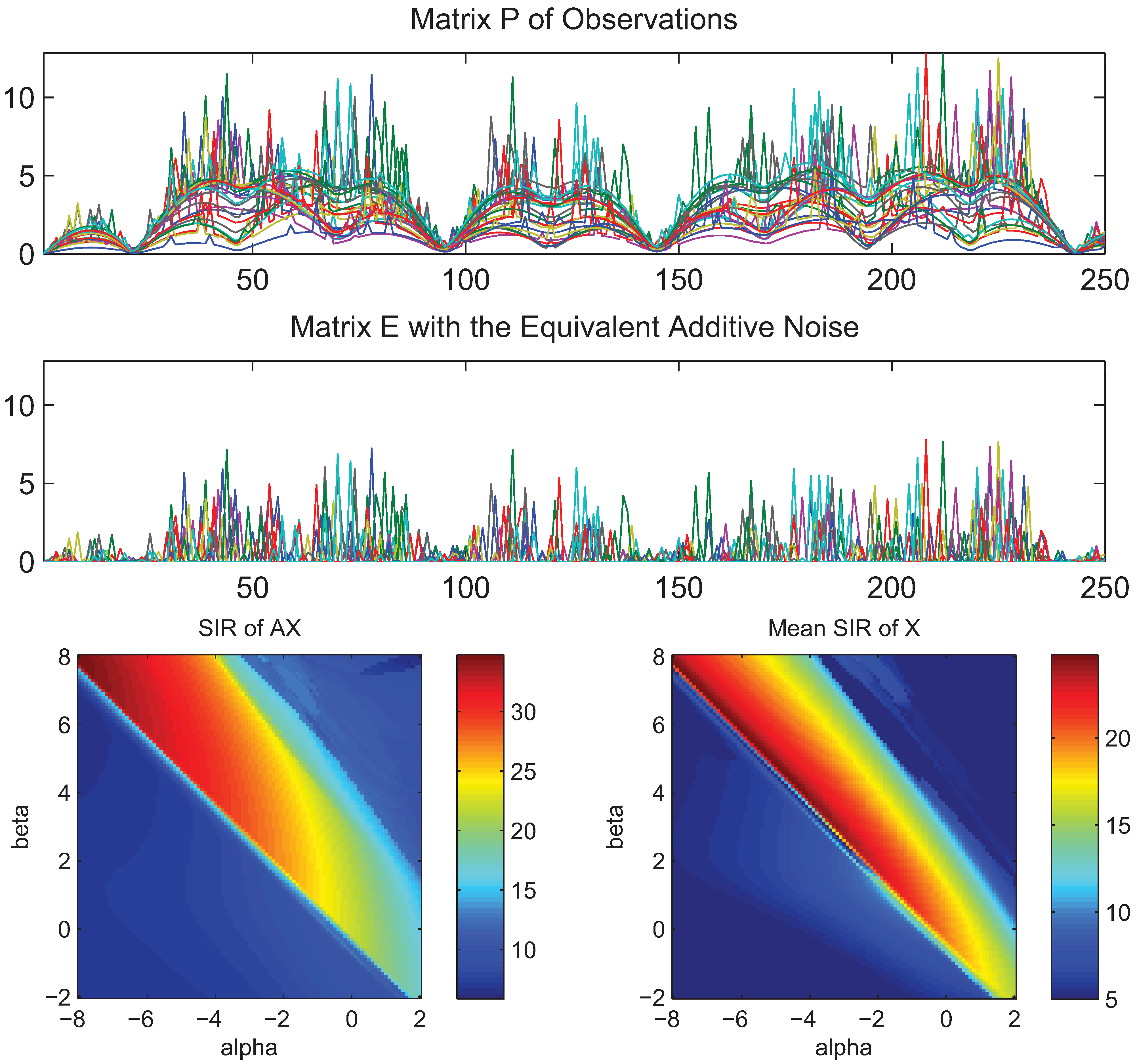
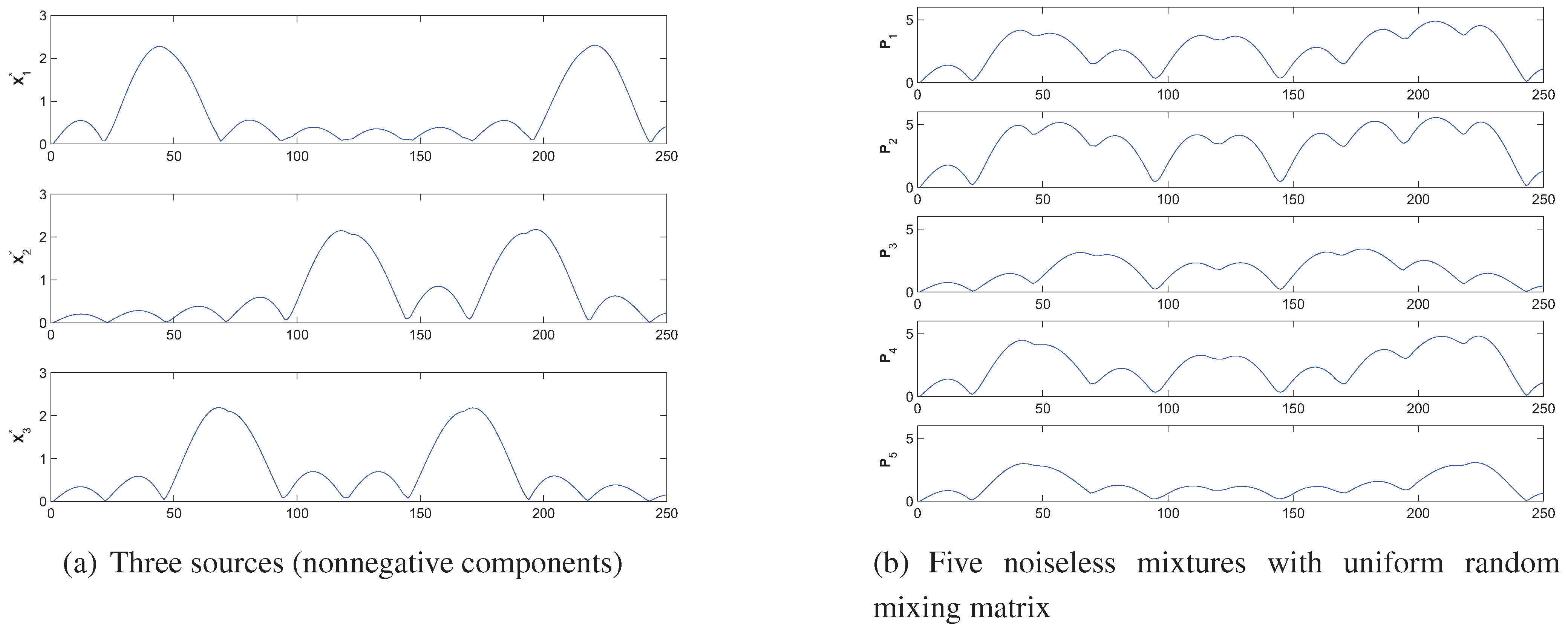
4. Simulations and Experimental Results

We have conducted extensive simulations with experiments designed specifically to address the following aspects:
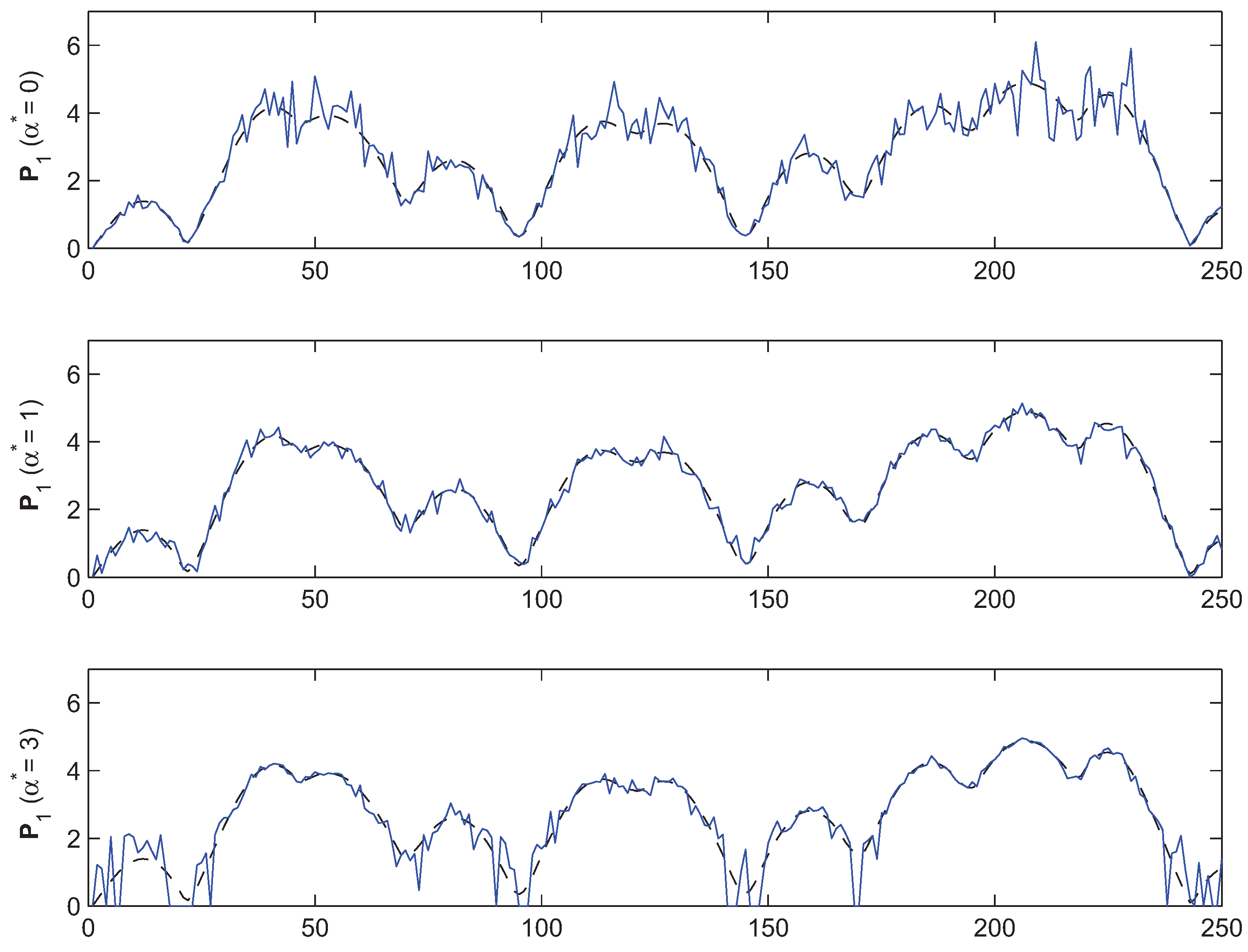
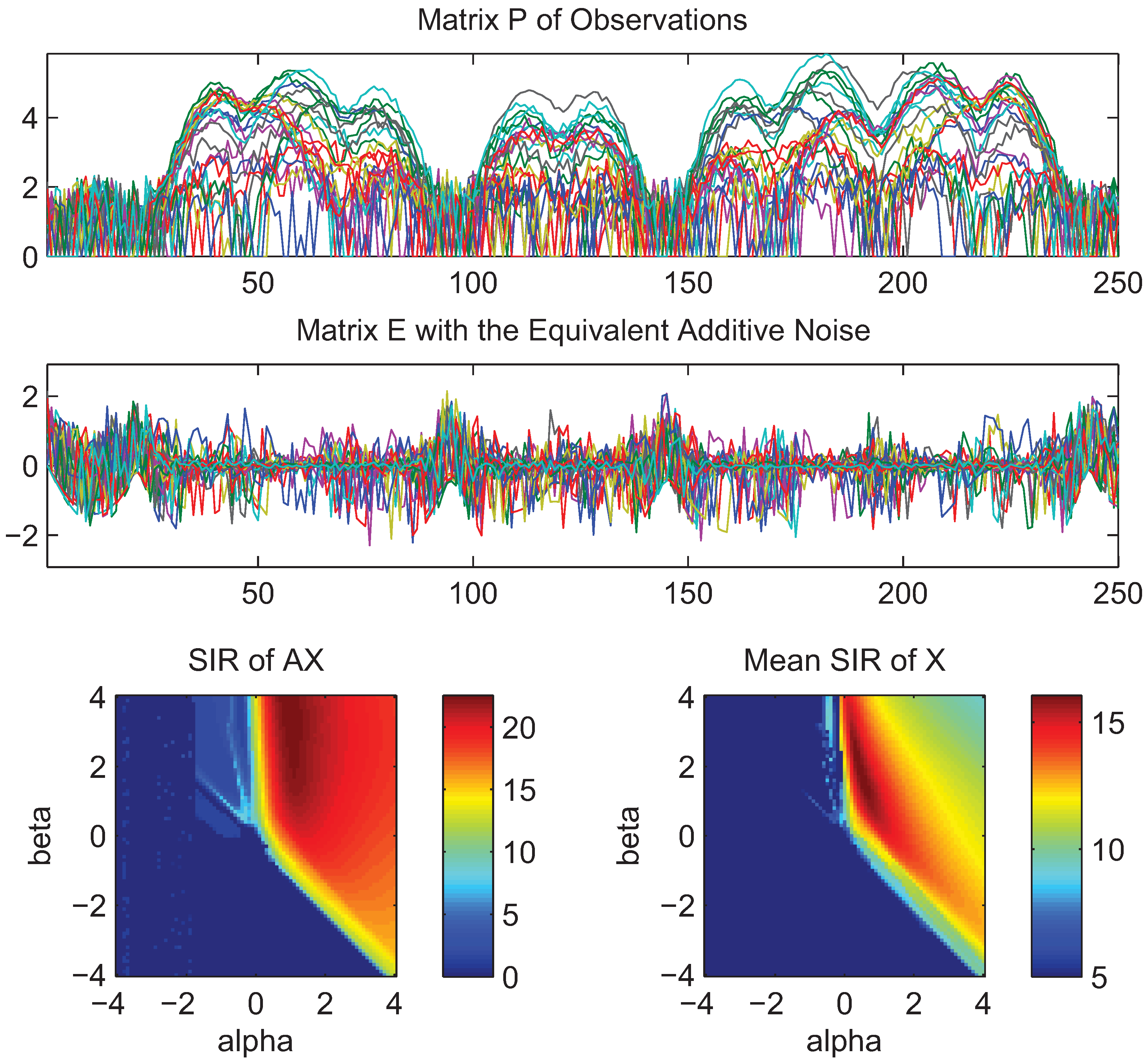
  • What is approximately a range of parameters alpha and beta for which the AB-multiplicative NMF algorithm exhibits the balance between relatively fastest convergence and good performance.
  • What is approximately the range of parameters of alpha and beta for which the AB-multiplicative NMF algorithm provides a stable solution independent of how many iterations are needed.
  • How robust is the AB-multiplicative NMF algorithm to noisy mixtures under multiplicative Gaussian noise, additive Gaussian noise, spiky biased noise? In other words, find a reasonable range of parameters for which the AB-multiplicative NMF algorithm gives improved performance when the data are contaminated by the different types of noise.
In order to test the performance of the AB-divergence for the NMF problem, we considered the matrix X * with three non-negative sources (rows) shown in Figure 7(a). These sources were obtained by superposing pairs of signals from the “ACsincpos10” benchmark of the NMFLAB toolbox and truncating their length to the first 250 samples [7]. We mix these sources with a random mixing matrix A * of dimension 25 × 5 , whose elements were drawn independently from a uniform random distribution in the unit interval. This way, we obtain a noiseless observation matrix P = A * X * whose first five rows are displayed in Figure 7(b).
Figure 7. Illustration of simulation experiments with three nonnegative sources and their typical mixtures using a randomly generated (uniformly distributed) mixing matrix (rows of a data matrix P = A X + E are denoted by p 1 , p 2 , . . . ).
Entropy 13 00134 g007
Our objective is to reconstruct from the noisy data P , the matrix X of the nonnegative sources and the mixing matrix A , by ignoring the scaling and permutation ambiguities.
The performance was evaluated with the mean Signal to Interference Ratio (SIR) of the estimated factorization model A X and the mean SIR of the estimated sources (the rows of the X ) [7].
We evaluate the proposed NMF algorithm in (61) based on the AB-divergence for very large number of pairs of values of ( α , β ) , and a wide range of their values. The algorithm used a single trial random initialization, followed by a refinement which consist of running ten initial iterations of the algorithm with ( α , β ) = ( 0 . 5 , 0 . 5 ) . This initialization phase serves to approach the model to the observations ( A X P ) which is important for guaranteing the posterior monotonic descent in the divergence when the parameters are arbitrary, as discussed in Section 3.3. Then, we ran only 250 iterations of the proposed NMF algorithm for the selected pair of parameters ( α , β ) .
To address the influence of noise, the observations were modeled as P = Q * + E , where Q * = A * X * and E denote, respectively, the desired components and the additive noise. To cater for different types of noises, we assume that the elements of the additive noise e i t are functions of the noiseless model q i t * and of another noise z i t , which was independent of q i t * . Moreover, we also assume that the signal q i t * and the noise z i t combine additively to give the observations in the deformed logarithm domain as
ln 1 α * ( p i t ) = ln 1 α * ( q i t * ) + ln 1 α * ( z i t ) ,
which is controlled by the parameter α * . Solving for the observations, we obtain
p i t = exp 1 α * ln 1 α * ( q i t * ) + ln 1 α * ( z i t ) .
or equivalently,
p i t = l l q i t * z i t , α * = 0 , multiplicative noise , q i t * + z i t , α * = 1 , additive noise , ( q i t * ) α * + ( z i t ) α * 1 α * , α * 0 , additive noise in a deformed log-domain .
Such approach allows us to model, under one single umbrella, noises of multiplicative type, additive noises, and other noises that act additively in a transformed domain, together with their distributions.
In order to generate the observations, we should assume first a probability density function g ( z ¯ i t ) for z ¯ i t ln 1 α * ( z i t ) , the noise in the transformed domain. This distribution is corrected, when necessary, to the nearby distribution that satisfies the positivity constraint of the observations.
In the following, we assume that the noise in the transformed domain z ¯ i t is Gaussian. Figure 8 presents mixtures obtained for this noise under different values of α * . The transformation (106) of the Gaussian density g ( z ¯ i t ) leads to the marginal distribution of the observations
f ( p i t | q i t * ) = 1 2 π σ p i t 1 α * e ln 1 α * ( p i t ) ln 1 α * ( q i t * ) 2 2 σ 2 , p i t > 0 ,
which can be recognized as a deformed log-Gaussian distribution (of order 1 α * ), with mean ln 1 α * ( q i t * ) and variance σ 2 . This distribution is exact for multiplicative noise ( α * = 0 ), since in this case no correction of the distribution is necessary to guarantee the non-negativity of the observations. For the remaining cases the distribution is only approximate, but the approximation improves when α * is not far from zero or when q i t * is sufficient large for all i , t , and for σ 2 sufficient small.
Figure 8. Illustration of the effect of the parameter α * on the noisy observations ( p 1 denotes the first row of the matrix P ). Dashed lines corresponds to noiseless mixtures and solid lines to the noisy mixtures that obtained when adding noise in the deformed logarithm ( ln 1 α * ( · ) ) domain. The noise distribution was Gaussian of zero mean and with a variance chosen so as to obtain an SNR of 20 dB in the deformed logarithm domain. In the top panel the value of the deformation parameter α * = 0 , resulting a multiplicative noise that distorts more strongly signals q i t * with larger values. For the middle panel α * = 1 , resulting in an additive Gaussian noise that equally affects all q i t * independently of their values. For the bottom panel, α * = 3 , distorting more strongly small values of q i t * .
Entropy 13 00134 g008
Interestingly, the log-likelihood of the matrix of observations for mutually independent components, distributed according to (108), is
ln f ( P | Q ) = i , t ln 2 π σ p i t 1 α * 1 σ 2 D A B ( α * , α * ) ( P Q ) .
Therefore, provided that (108) is sufficiently accurate, the maximization of the likelihood of the observations is equivalent to the minimization of the AB-divergence for ( α * , α * ) , that is,
arg max Q ln f ( P | Q ) arg min Q D A B ( α * , α * ) ( P Q ) .
Figure 9 presents the simulation results for mixtures with multiplicative noise. Usually, performances with SIR > 15 dB are considered successful. Observe that the domain where the performance is satisfactory is restricted to α + β 0 . 5 , otherwise some terms could be extremely small due the inversion of the arguments of the AB-divergence. In other words, for α + β < 0 . 5 there is too strong enhancement of the observations that correspond to the values of the model close to zero, deteriorating the performance. In our simulations we restricted the minimum value of entries of the true factorization model to a very small value of 10 7 .
Figure 9. Performance of the AB-multiplicative NMF algorithm in the presence of multiplicative noise ( α * = 0 ). The distribution of the noise in the transformed domain z ¯ i t is Gaussian of zero mean and with variance set to obtain an SNR of 20 dB in the ln ( · ) domain. The rows of the observation matrix are shown in the top panel, the equivalent additive noise E = P Q * is displayed at the middle panel and the performance results are presented at the bottom panels. As theoretically expected, the best SIR of the model ( 26 . 7 dB) was achieved in the neighborhood of ( 0 , 0 ) , the parameters for which the likelihood of these observations is maximized. On the other hand, the best mean SIR of the sources ( 18 . 0 dB) and of the mixture ( 21 . 1 dB) are both obtained for ( α , β ) close to ( 1 . 0 , 1 . 0 ) .
Entropy 13 00134 g009
We confirmed this by extensive computer simulations. As theoretically predicted, for a Gaussian distribution of the noise z ¯ i t with α * = 0 , the best performance in the reconstruction of desired components was obtained in the neighborhood of the origin of the ( α , β ) plane. The generalized Itakura-Saito divergence of Equation (46) gives usually a reasonable or best performance for the estimation of X and A . The result of the simulation can be interpreted in light of the discussion presented in Section 2.3. As the multiplicative noise increases the distortion at large values of the model, the best performance was obtained for those parameters that prevent the inversion of the arguments of the divergence and, at the same time, suppress the observations that correspond with larger values of the model. This leads to the close to optimal choice of the parameters that satisfy equation α + β = 0 .
The performance for the case of additive Gaussian noise ( α * = 1 ) is presented in Figure 10. For an SNR of 20 dB, the distribution of the noisy observations was approximately Gaussian, since only 1 % of the coordinates of the matrix P were rectified to enforce positivity. This justifies the best performance for the NMF model in the neighborhood of the pair ( α , β ) = ( 1 , 1 ) , since according to (110) minimizing this divergence approximately maximizes the likelihood of these observations. Additionally, we observed poor performance for negative values of α, explained by the large ratios p i t / q i t being much more unreliable, due to the distortion of the noise for the small values of q i t * , together with the rectifying of the negative observations.
Figure 10. Performance of the AB-multiplicative NMF algorithm for 25 mixtures with additive Gaussian noise and SNR of 20 dB. The best performance for A X was for an SIR of 31 . 1 dB, obtained for ( α , β ) = ( 0 . 8 , 0 . 7 ) , that is, close to the pair ( 1 , 1 ) that approximately maximizes the likelihood of the observations. The best performance for X and A was obtained in the vicinity of ( 0 . 2 , 0 . 8 ) , with respective mean SIRs of 17 . 7 dB and 20 . 5 dB.
Entropy 13 00134 g010
Figure 11 shows simulation results with α * = 3 , the case for which the effect of the noise was more pronounced for the small values of q i t * . The noise in the transformed domain was again Gaussian and set to an SNR (in this domain) of 20 dB. In this case, the distribution of the observation was no longer sufficiently close to Gaussian because 11 % of the entries of the matrix P were rectified to enforce their positivity. The graphs reveal that the best performance was obtained for the pair ( α , β ) = ( 0 . 9 , 4 . 0 ) that is quite close to a Beta-divergence. As a consequence of the strong distortion by the noise the small values of the factorization model the large and small ratios p i t / q i t were not reliable, leaving as preferable the values of α close to unity. On the other hand, the ratios associated with small q i t should be penalized, what leads to a larger parameter β as a robust choice against the contamination of the small values of the model.
Figure 11. Performance of the AB-multiplicative NMF algorithm when the observations are contaminated with Gaussian noise in the ln 1 α * ( · ) domain, for α * = 3 . The best performance for A X was for an SIR of 22 . 6 dB obtained for ( α , β ) = ( 0 . 9 , 4 . 0 ) . A best SIR of 16 . 1 dB for X was obtained for ( α , β ) = ( 0 . 5 , 1 . 7 ) , which gave an SIR for A of 19 . 1 dB.
Entropy 13 00134 g011
The last two simulations, shown in Figure 12 and Figure 13, illustrate the effect of uniform spiky noise which was activated with a probability of 0 . 1 and contained a bias in its mean. When the observations are biased downwards by the noise the performance improves for a positive α since, as Figure 3 illustrates, in this case the α suppresses the smaller ratios p i t / q i t . On the other hand, for a positive bias we have the opposite effect, resulting in the negative values of α being preferable. With these changes in α, the value of β should be modified accordingly to be in the vicinity of α plus a given offset, so as to avoid an excessive penalty for observations that correspond to the large or small values of the factorization model q i t .
Figure 12. Performance for biased (non-zero mean) and spiky, additive noise. For α * = 1 , we have uniform noise with support in the negative unit interval, which is a spiky or sparse in the sense that it is only activated with a probability of 0 . 1 , i.e., it corrupts only 10 % of observed samples. The best SIR results were obtained around the line ( α , 1 α ) for both positive and large values of α.
Entropy 13 00134 g012
Figure 13. Performance for multiplicative noise that is positively biased and spiky (activated with a probability of 0 . 1 ). For α * = 0 , the noise in the ln ( · ) domain ( z ¯ i t ) followed a uniform distribution with support in the unit interval. The best SIR results were obtained along the line ( α , α ) for negative values of α.
Entropy 13 00134 g013

5. Conclusions

We have introduced the generalized Alpha-Beta divergence which serves as a flexible and robust cost function and forms a basis for the development of a new class of generalized multiplicative algorithms for NMF. Natural extensions of the Lee-Seung, ISRA, EMML and other NMF algorithms have been presented, in order to obtain more flexible and robust solutions with respect to different contaminations of the data by noise. This class of algorithms allows us to reconstruct (recover) the original signals and to estimate the mixing matrices, even when the observed data are imprecise and/or corrupted by noise. The optimal choice of the tuning parameters α and β depends strongly both on the distribution of noise and the way it contaminates the data. However, it should be emphasized that we are not expecting that the AB-multiplicative NMF algorithms proposed in this paper will work well for any set of parameters.
In summary, we have rigorously derived a new family of robust AB-multiplicative NMF algorithms using the generalized Alpha-Beta Divergence which unifies and extends a number of the existing divergences. The proposed AB-multiplicative NMF algorithms have been shown to work for wide sets of parameters and combine smoothly many existing NMF algorithms. Moreover, they are also adopted for large-scale low-rank approximation problems. Extensive simulation results have confirmed that the developed algorithms are efficient, robust and stable for a wide range of parameters. The proposed algorithms can also be extended to Nonnegative Tensor Factorizations and Nonnegative Tucker Decompositions in a straightforward manner.

References

  1. Amari, S. Differential-Geometrical Methods in Statistics; Springer Verlag: New York, NY, USA, 1985. [Google Scholar]
  2. Amari, S. Dualistic geometry of the manifold of higher-order neurons. Neural Network. 1991, 4, 443–451. [Google Scholar] [CrossRef]
  3. Amari, S.; Nagaoka, H. Methods of Information Geometry; Oxford University Press: New York, NY, USA, 2000. [Google Scholar]
  4. Amari, S. Integration of stochastic models by minimizing α-divergence. Neural Comput. 2007, 19, 2780–2796. [Google Scholar] [CrossRef] [PubMed]
  5. Amari, S. Information geometry and its applications: Convex function and dually flat manifold. In Emerging Trends in Visual Computing; Nielsen, F., Ed.; Springer Lecture Notes in Computer Science: Palaiseau, France, 2009a; Volume 5416, pp. 75–102. [Google Scholar]
  6. Amari, S.; Cichocki, A. Information geometry of divergence functions. Bull. Pol. Acad. Sci. Math. 2010, 58, 183–195. [Google Scholar] [CrossRef]
  7. Cichocki, A.; Zdunek, R.; Phan, A.H.; Amari, S. Nonnegative Matrix and Tensor Factorizations; John Wiley & Sons Ltd.: Chichester, UK, 2009. [Google Scholar]
  8. Cichocki, A.; Zdunek, R.; Amari, S. Csiszár’s divergences for nonnegative matrix factorization: Family of new algorithms. In Lecture Notes in Computer Science; Springer: Charleston, SC, USA, 2006; Volume 3889, pp. 32–39. [Google Scholar]
  9. Kompass, R. A Generalized divergence measure for nonnegative matrix factorization. Neural Comput. 2006, 19, 780–791. [Google Scholar] [CrossRef] [PubMed]
  10. Dhillon, I.; Sra, S. Generalized nonnegative matrix approximations with Bregman divergences. Neural Inform. Process. Syst. 2005, 283–290. [Google Scholar]
  11. Amari, S. α-divergence is unique, belonging to both f-divergence and Bregman divergence classes. IEEE Trans. Inform. Theor. 2009b, 55, 4925–4931. [Google Scholar] [CrossRef]
  12. Murata, N.; Takenouchi, T.; Kanamori, T.; Eguchi, S. Convergence-guaranteed multi U-Boost and Bregman divergence. Neural Comput. 2004, 16, 1437–1481. [Google Scholar] [CrossRef] [PubMed]
  13. Fujimoto, Y.; Murata, N. A modified EM Algorithm for mixture models based on Bregman divergence. Ann. Inst. Stat. Math. 2007, 59, 57–75. [Google Scholar] [CrossRef]
  14. Zhu, H.; Rohwer, R. Bayesian invariant measurements of generalization. Neural Process. Lett. 1995, 2, 28–31. [Google Scholar] [CrossRef]
  15. Zhu, H.; Rohwer, R. Measurements of generalisation based on information geometry. In Mathematics of Neural Networks: Model Algorithms and Applications; Ellacott, S.W., Mason, J.C., Anderson, I.J., Eds.; Kluwer: Norwell, MA, USA, 1997; pp. 394–398. [Google Scholar]
  16. Nielsen, F.; Nock, R. Sided and symmetrized Bregman centroids. IEEE Trans. Inform. Theor. 2009, 56, 2882–2903. [Google Scholar] [CrossRef]
  17. Boissonnat, J.D.; Nielsen, F.; Nock, R. Bregman Voronoi diagrams. Discrete Comput. Geom. 2010, 44, 281–307. [Google Scholar] [CrossRef]
  18. Yamano, T. A generalization of the Kullback-Leibler divergence and its properties. J. Math. Phys. 2009, 50, 85–95. [Google Scholar] [CrossRef]
  19. Minami, M.; Eguchi, S. Robust blind source separation by Beta-divergence. Neural Comput. 2002, 14, 1859–1886. [Google Scholar]
  20. Bregman, L. The relaxation method of finding a common point of convex sets and its application to the solution of problems in convex programming. Comp. Math. Phys. USSR 1967, 7, 200–217. [Google Scholar] [CrossRef]
  21. Csiszár, I. Eine Informations Theoretische Ungleichung und ihre Anwendung auf den Beweiss der Ergodizität von Markoffschen Ketten. Magyar Tud. Akad. Mat. Kutató Int. Közl 1963, 8, 85–108. [Google Scholar]
  22. Csiszár, I. Axiomatic characterizations of information measures. Entropy 2008, 10, 261–273. [Google Scholar] [CrossRef]
  23. Csiszár, I. Information measures: A critial survey. In Proceedings of the Transactions of the 7th Prague Conference, Prague, Czechoslovakia, 18–23 August 1974; pp. 83–86.
  24. Ali, M.; Silvey, S. A general class of coefficients of divergence of one distribution from another. J. Roy. Stat. Soc. 1966, Ser B, 131–142. [Google Scholar]
  25. Hein, M.; Bousquet, O. Hilbertian metrics and positive definite kernels on probability measures. In Proceedings of the Tenth International Workshop on Artificial Intelligence and Statistics, Barbados, 6–8 January 2005; pp. 136–143.
  26. Zhang, J. Divergence function, duality, and convex analysis. Neural Comput. 2004, 16, 159–195. [Google Scholar] [CrossRef] [PubMed]
  27. Zhang, J.; Matsuzoe, H. Dualistic differential geometry associated with a convex function. In Springer Series of Advances in Mechanics and Mathematics; 2008; Springer: New York, NY, USA; pp. 58–67. [Google Scholar]
  28. Lafferty, J. Additive models, boosting, and inference for generalized divergences. In Proceedings of the Twelfth Annual Conference on Computational Learning Theory (COLT’99), Santa Cruz, CA, USA, 7-9 July 1999.
  29. Banerjee, A.; Merugu, S.; Dhillon, I.S.; Ghosh, J. Clustering with Bregman divergences. J. Mach. Learn. Res. 2005, 6, 1705–1749. [Google Scholar]
  30. Villmann, T.; Haase, S. Divergence based vector quantization using Fréchet derivatives. Neural Comput. 2011, in press. [Google Scholar]
  31. Villmann, T.; Haase, S.; Schleif, F.M.; Hammer, B. Divergence based online learning in vector quantization. In Proceedings of the International Conference on Artifial Intelligence and Soft Computing (ICAISC’2010), LNAI, Zakopane, Poland, 13–17 June 2010.
  32. Cichocki, A.; Amari, S.; Zdunek, R.; Kompass, R.; Hori, G.; He, Z. Extended SMART algorithms for nonnegative matrix factorization. In Lecture Notes in Artificial Intelligence; Springer: Zakopane, Poland, 2006; Volume 4029, pp. 548–562. [Google Scholar]
  33. Cichocki, A.; Zdunek, R.; Choi, S.; Plemmons, R.; Amari, S. Nonnegative tensor factorization using Alpha and Beta divergences. In IEEE International Conference on Acoustics, Speech, and Signal Processing, Honolulu, Hawaii, USA, 15–20 April 2007; Volume III, pp. 1393–1396.
  34. Cichocki, A.; Zdunek, R.; Choi, S.; Plemmons, R.; Amari, S.I. Novel multi-layer nonnegative tensor factorization with sparsity constraints. In Lecture Notes in Computer Science; Springer: Warsaw, Poland, 2007; Volume 4432, pp. 271–280. [Google Scholar]
  35. Cichocki, A.; Amari, S. Families of Alpha- Beta- and Gamma- divergences: Flexible and robust measures of similarities. Entropy 2010, 12, 1532–1568. [Google Scholar] [CrossRef]
  36. Paatero, P.; Tapper, U. Positive matrix factorization: A nonnegative factor model with optimal utilization of error estimates of data values. Environmetrics 1994, 5, 111–126. [Google Scholar] [CrossRef]
  37. Lee, D.; Seung, H. Learning of the parts of objects by non-negative matrix factorization. Nature 1999, 401, 788–791. [Google Scholar] [PubMed]
  38. Lee, D.; Seung, H. Algorithms for Nonnegative Matrix Factorization; MIT Press: Cambridge MA, USA, 2001; Volume 13, pp. 556–562. [Google Scholar]
  39. Gillis, N.; Glineur, F. Nonnegative factorization and maximum edge biclique problem. ECORE discussion paper 2010. 106 (also CORE DP 2010/59). Available online: http://www.ecore.be/DPs/dp_1288012410.pdf (accessed on 1 November 2008).
  40. Daube-Witherspoon, M.; Muehllehner, G. An iterative image space reconstruction algorthm suitable for volume ECT. IEEE Trans. Med. Imag. 1986, 5, 61–66. [Google Scholar] [CrossRef] [PubMed]
  41. De Pierro, A. On the relation between the ISRA and the EM algorithm for positron emission tomography. IEEE Trans. Med. Imag. 1993, 12, 328–333. [Google Scholar] [CrossRef] [PubMed]
  42. De Pierro, A.R. A Modified expectation maximization algorithm for penalized likelihood estimation in emission tomography. IEEE Trans. Med. Imag. 1995, 14, 132–137. [Google Scholar] [CrossRef] [PubMed]
  43. De Pierro, A.; Yamagishi, M.B. Fast iterative methods applied to tomography models with general Gibbs priors. In Proceedings of the SPIE Technical Conference on Mathematical Modeling, Bayesian Estimation and Inverse Problems, Denver, CO, USA, 21 July 1999; Volume 3816, pp. 134–138.
  44. Lantéri, H.; Roche, M.; Aime, C. Penalized maximum likelihood image restoration with positivity constraints: multiplicative algorithms. Inverse Probl. 2002, 18, 1397–1419. [Google Scholar] [CrossRef]
  45. Byrne, C. Accelerating the EMML algorithm and related iterative algorithms by rescaled block-iterative (RBI) methods. IEEE Trans. Med. Imag. 1998, IP-7, 100–109. [Google Scholar] [CrossRef] [PubMed]
  46. Lewitt, R.; Muehllehner, G. Accelerated iterative reconstruction for positron emission tomography based on the EM algorithm for maximum-likelihood estimation. IEEE Trans. Med. Imag. 1986, MI-5, 16–22. [Google Scholar] [CrossRef] [PubMed]
  47. Byrne, C. Signal Processing: A Mathematical Approach; A.K. Peters, Publ.: Wellesley, MA, USA, 2005. [Google Scholar]
  48. Shepp, L.; Vardi, Y. Maximum likelihood reconstruction for emission tomography. IEEE Trans. Med. Imag. 1982, MI-1, 113–122. [Google Scholar] [CrossRef] [PubMed]
  49. Kaufman, L. Maximum likelihood, least squares, and penalized least squares for PET. IEEE Trans. Med. Imag. 1993, 12, 200–214. [Google Scholar] [CrossRef] [PubMed]
  50. Lantéri, H.; Soummmer, R.; Aime, C. Comparison between ISRA and RLA algorithms: Use of a Wiener filter based stopping criterion. Astron. Astrophys. Suppl. 1999, 140, 235–246. [Google Scholar] [CrossRef]
  51. Cichocki, A.; Zdunek, R.; Amari, S.I. Hierarchical ALS algorithms for nonnegative matrix and 3D tensor factorization. In Lecture Notes on Computer Science; Springer: London, UK, 2007; Volume 4666, pp. 169–176. [Google Scholar]
  52. Minka, T. Divergence measures and message passing. In Microsoft Research Technical Report; MSR-TR-2005-173; Microsoft Research Ltd.: Cambridge, UK, 7 December 2005. [Google Scholar]
  53. Févotte, C.; Bertin, N.; Durrieu, J.L. Nonnegative matrix factorization with the Itakura-Saito divergence with application to music analysis. Neural Comput. 2009, 21, 793–830. [Google Scholar] [CrossRef] [PubMed]
  54. Itakura, F.; Saito, F. Analysis synthesis telephony based on the maximum likelihood method. In Proceedings of the 6th International Congress on Acoustics, Tokyo, Japan, 21–28 August 1968; pp. 17–20.
  55. Basu, A.; Harris, I.R.; Hjort, N.; Jones, M. Robust and efficient estimation by minimising a density power divergence. Biometrika 1998, 85, 549–559. [Google Scholar] [CrossRef]
  56. Jones, M.; Hjort, N.; Harris, I.R.; Basu, A. A comparison of related density-based minimum divergence estimators. Biometrika 1998, 85, 865–873. [Google Scholar] [CrossRef]
  57. Kivinen, J.; Warmuth, M. Exponentiated gradient versus gradient descent for linear predictors. Inform. Comput. 1997, 132, 1–63. [Google Scholar] [CrossRef]
  58. Cichocki, A.; Lee, H.; Kim, Y.D.; Choi, S. Nonnegative matrix factorization with α-divergence. Pattern Recogn. Lett. 2008, 29, 1433–1440. [Google Scholar] [CrossRef]
  59. Févotte, C.; Idier, J. Algorithms for nonnegative matrix factorization with the β-divergence. Technical Report arXiv 2010. Available online: http://arxiv.org/abs/1010.1763 (accessed on 13 October 2010).
  60. Nakano, M.; Kameoka, H.; Le Roux, J.; Kitano, Y.; Ono, N.; Sagayama, S. Convergence-guaranteed multiplicative algorithms for non-negative matrix factorization with β-divergence. In Proceedings of the 2010 IEEE International Workshop on Machine Learning for Signal Processing (MLSP), Kittila, Finland, 29 August–1 September 2010; pp. 283–288.
  61. Badeau, R.; Bertin, N.; Vincent, E. Stability analysis of multiplicative updates algorithms and application to nonnegative matirx factroization. IEEE Trans. Neural Network. 2010, 21, 1869–1881. [Google Scholar] [CrossRef] [PubMed]
  62. Favati, P.; Lotti, G.; Menchi, O.; Romani, F. Performance analysis of maximum likelihood methods for regularization problems with nonnegativity constraints. Inverse Probl. 2010, 28, 85013–85030. [Google Scholar] [CrossRef]
  63. Benvenuto, F.; Zanella, R.; Zanni, L.; Bertero, M. Nonnegative least-squares image deblurring: Improved gradient projection approaches. Inverse Probl. 2010, 26, 25004–25021. [Google Scholar] [CrossRef]

Appendix

A. Non-negativity of the AB-divergence

In this appendix we prove that AB-divergence is nonnegative for any values of α and β, and is equal to zero if and only if P = Q .
For any nonnegative real numbers x and y, and for any positive real numbers a and b that are Hölder conjugate i.e., a 1 + b 1 = 1 , Young’s inequality states that
x y x a a + y b b ,
with equality only for x a = y b .
We shall now show how the non-negativity of the proposed divergence rest on three different inequalities of the Young’s type, each one holding true for a different combination of the signs of the constants: α β , α ( α + β ) and β ( α + β ) .
For α β > 0 , α ( α + β ) > 0 and β ( α + β ) > 0 , we set x = p i t α , y = q i t β , a = ( α + β ) / α and b = ( α + β ) / β , to obtain
1 α β p i t α q i t β 1 α β ( p i t α ) α + β α ( α + β ) α + ( q i t β ) α + β β ( α + β ) β = 1 α β α ( α + β ) p i t α + β + β ( α + β ) q i t α + β .
For α β < 0 , α ( α + β ) > 0 and β ( α + β ) < 0 we set x = p i t α + β q i t β ( α + β ) α , y = q i t β ( α + β ) α , a = α / ( α + β ) and b = α / β , to obtain
1 β ( α + β ) p i t α + β 1 β ( α + β ) p i t α + β q i t β ( α + β ) α α α + β α α + β + q i t β ( α + β ) α α β α β = 1 α β p i t α q i t β + β ( α + β ) q i t ( α + β ) .
Finally, for α β < 0 , α ( α + β ) < 0 and β ( α + β ) > 0 we set x = p i t α ( α + β ) β q i t α + β , y = p i t α ( α + β ) β , a = β / ( α + β ) and b = β / α , to obtain
1 α ( α + β ) q i t α + β 1 α ( α + β ) p i t α ( α + β ) β q i t α + β β α + β β α + β + p i t α ( α + β ) β β α β α = 1 α β p i t α q i t β + α ( α + β ) p i t ( α + β ) .
The three considered cases exhaust all the possibilities for the sign of the constants: α β , α ( α + β ) and β ( α + β ) . Inequalities (112)-(114) can be summarized as the joint inequality:
1 α β p i t α q i t β 1 β ( α + β ) p i t α + β + 1 α ( α + β ) q i t α + β , for α , β , α + β 0 ,
where the equality holds only for p i t = q i t . This above inequality justifies the non-negativity of the divergence defined in (19).

B. Proof of the Conditional Auxiliary Function Character of G ( { Q ( k + 1 ) } , { Q ( k ) } ; P )

The factorization model of the observations Q ( k ) at a k-th iteration is a sum of rank-one matrices, so that
q i t ( k ) = j = 1 J a i j ( k ) x j t ( k ) = j = 1 J γ i t ( j ) ( { Q ( k ) } ) q i t ( k ) ,
where the parameter
γ i t ( j ) ( { Q ( k ) } ) = a i j ( k ) x j t ( k ) q i t ( k ) 0 ,
denotes the normalized contribution of the j th rank-one component to the model q i t ( k ) . For a given auxiliary function and since j γ i t ( j ) ( { Q ( k ) } ) = 1 , the elements of the matrix Q ( k + 1 ) resulting from the minimization in (75) can also be expressed by the convex sum
q i t ( k + 1 ) = j γ i t ( j ) ( { Q ( k ) } ) q ^ i t ( j ) where q ^ i t ( j ) = a i j ( k + 1 ) x j t ( k + 1 ) γ i t ( j ) ( { Q ( k ) } ) , j = 1 , 2 , , J .
In this context the q ^ i t ( j ) elements represent a prediction of q i t ( k + 1 ) obtained from the j th -rank-one component ( a i j ( k + 1 ) x j t ( k + 1 ) ), assuming that proportions of the components in the model are still governed by γ i t ( j ) ( { Q ( k ) } ) .
If, additionally, the convexity of d A B ( α , β ) ( p i t , q ^ i t ) w.r.t. the second argument holds true in the interval [ min j q ^ i t ( j ) , max j q ^ i t ( j ) ] and for each i , t , the function
G ( { Q ( k + 1 ) } , { Q ( k ) } ; P ) = i , t j γ i t ( j ) ( { Q ( k ) } ) d A B ( α , β ) p i t , q ^ i t ( j ) ,
can be lower-bounded by means of Jensen’s inequality
i , t j γ i t ( j ) ( { Q ( k ) } ) d A B ( α , β ) p i t , q ^ i t ( j ) i , t d A B ( α , β ) p i t , j γ i t ( j ) ( { Q ( k ) } ) q ^ i t ( j ) .
>From (118), observe that the previous lower bound is the AB-divergence
i , t d A B ( α , β ) p i t , j γ i t ( j ) ( { Q ( k ) } ) q ^ i t ( j ) = D A B ( α , β ) P | | Q ( k + 1 ) .
thus confirming that
G ( { Q ( k + 1 ) } , { Q ( k ) } ; P ) D A B ( α , β ) ( P | | Q ( k + 1 ) ) = G ( { Q ( k + 1 ) } , { Q ( k + 1 ) } ; P ) ,
and proving the desired result: G ( { Q ( k + 1 ) } , { Q ( k ) } ; P ) is an auxiliary function for the surrogate optimization of the AB-divergence provided that the convexity of d A B ( α , β ) ( p i t , q ^ i t ) for q ^ i t [ min j q ^ i t ( j ) , max j q ^ i t ( j ) ] and each i , t , is guaranteed at each iteration.

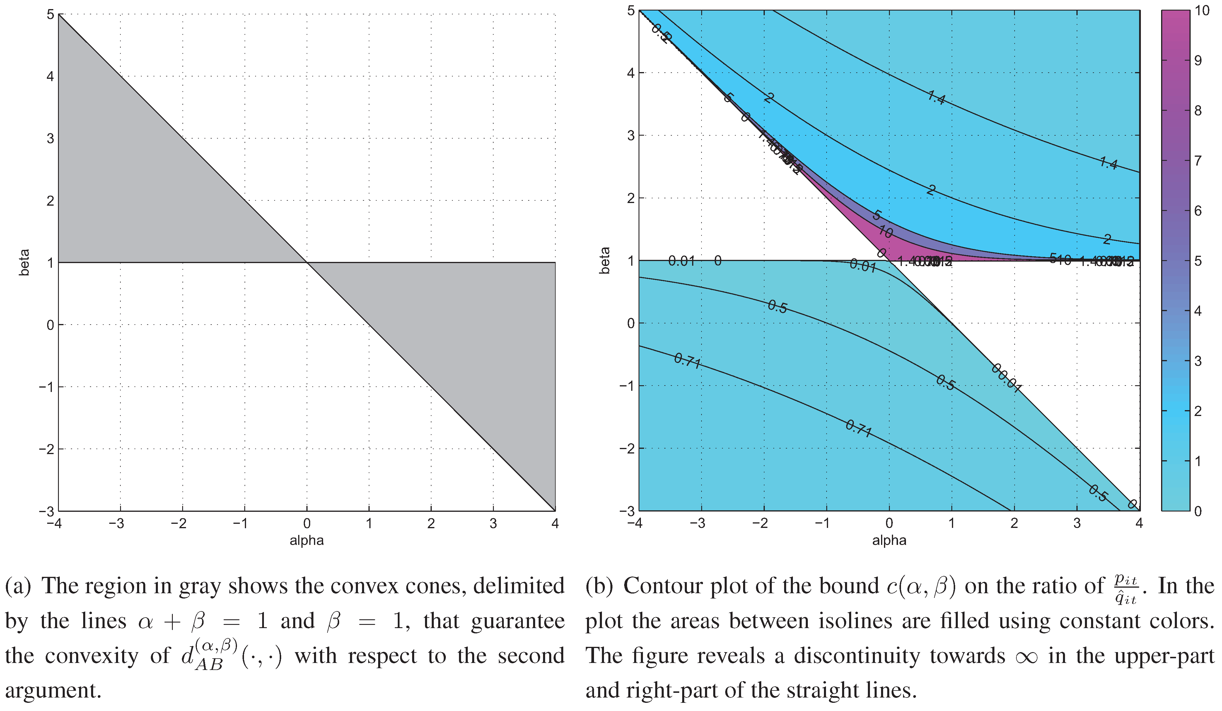
C. Necessary and Sufficient Conditions for Convexity

The convexity of the divergence with respect to the model (the second argument of the divergence) is an important property in the designing of update formulas with monotonic descent. The second order partial derivative of the divergence in (23) with respect to the second argument is given by
2 d A B ( α , β ) ( p i t , q i t ) q i t 2 = 1 + ( 1 β ) ln 1 α p i t q i t q i t α + β 2 .
For α = 0 , the proof of convexity for β = 1 is obvious from Equation (123). On the other hand, for α 0 , after the substitution of the deformed logarithm in (123) by its definition, a sufficient condition for the nonnegativity of the second partial derivative
2 d A B ( α , β ) ( p i t , q i t ) q i t 2 = 1 + 1 β α p i t q i t α 1 q i t α + β 2 ,
1 1 β α q i t α + β 2 ,
0 ,
is given by
1 β α [ 0 , 1 ] .
After combining the cases in a single expression the sufficient condition for the divergence d A B ( α , β ) ( p i t , q i t ) to be convex w.r.t. the second argument becomes
β [ min { 1 , 1 α } , max { 1 , 1 α } ] .
Figure 4(a) illustrates the domain where this sufficient condition is satisfied in the ( α , β ) plane.
We can continue further with the analysis to obtain the necessary and sufficient conditions for the convexity after solving directly (123). Depending on the value of β, one of the following conditions should be satisfied
p i t q i t c ( α , β ) for β < min { 1 , 1 α } , always convex for β [ min { 1 , 1 α } , max { 1 , 1 α } ] , p i t q i t c ( α , β ) for β > max { 1 , 1 α } ,
where the upper and lower bounds depend on the function
c ( α , β ) = exp 1 α 1 β 1 .
A contour plot of c ( α , β ) is shown in Figure 4(b).

