Finite-Time Thermoeconomic Optimization of a Solar-Driven Heat Engine Model

Abstract

In the present paper, the thermoeconomic optimization of an irreversible solar-driven heat engine model has been carried out by using finite-time/finite-size thermodynamic theory. In our study we take into account losses due to heat transfer across finite time temperature differences, heat leakage between thermal reservoirs and internal irreversibilities in terms of a parameter which comes from the Clausius inequality. In the considered heat engine model, the heat transfer from the hot reservoir to the working fluid is assumed to be Dulong-Petit type and the heat transfer to the cold reservoir is assumed of the Newtonian type. In this work, the optimum performance and two design parameters have been investigated under two objective functions: the power output per unit total cost and the ecological function per unit total cost. The effects of the technical and economical parameters on the thermoeconomic performance have been also discussed under the aforementioned two criteria of performance.

1. Introduction

In 2000, Sahin et al. [1] studied the thermoeconomic performance of an endoreversible solar-driven heat engine. In this study, they considered that the heat transfer from the hot reservoir to the working fluid is dominated by radiation because radiation heat transfer plays a key role in the collector ambient heat loss mechanism, while the mode of heat transfer from the working fluid to the cold reservoir is given by a Newtonian heat transfer law. Sahin et al. [1] calculated the optimum temperatures of the working fluid and the optimum efficiency of the engine operating at maximum power conditions. Later, Sahin and Kodal [2], applied this procedure to study the thermoeconomics of an endoreversible heat engine in terms of the maximization of a profit function defined as the quotient of the power output and the annual investment cost. Recently, Barranco-Jiménez et al. [3], studied the optimum operation conditions of an endoreversible heat engine with different heat transfer laws at the thermal couplings but operating under maximum ecological function conditions, and more recently, Barranco-Jiménez et al. [4] also studied the thermoeconomic optimum operation conditions of a solar-driven heat engine. In these studies, Barranco-Jiménez et al. considered three regimes of performance: The maximum power regime (MPR) [5,6,7], the maximum efficient power [8,9] and the maximum ecological function regime (MER) [10,11]. In this work, we study the thermoeconomics of an irreversible heat engine by considering further with losses due to heat transfer across finite time temperature differences [12,13,14,15], heat leakage between thermal reservoirs [16,17,18,19,20,21,22,23,24] and internal irreversibilities [25,26,27] in terms of a parameter which comes from the Clausius inequality. In our study we use two regimes of performance: The maximum power regime, and the so-called ecological function regime. Besides, in our thermoeconomical analysis, conductive-convective and radiative terms are considered by means of a heat transfer law of the Dulong-Petit type [28,29]. Some of our numerical results are compared with data stemming from three power plants [7,30]. The article is organizes as follows: In Section 2 we present the heat engine model; in Section 3 the numerical results and discussion are presented; finally in Section 4 we give the conclusions.

2. Theoretical Model

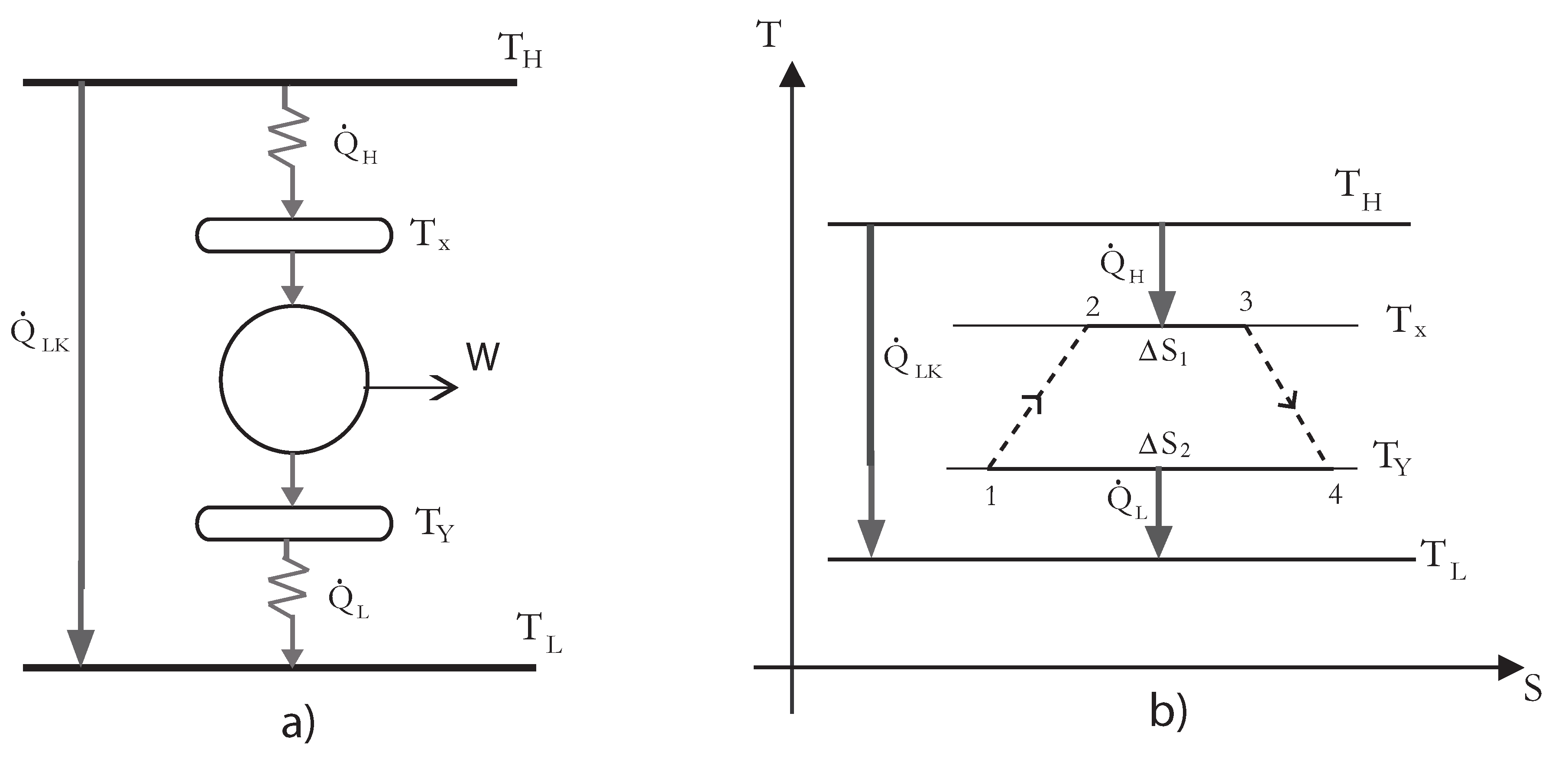
The considered irreversible solar-driven heat engine operates between a heat source of temperature $T_H$ (the collector) and a heat sink of temperature $T_L$ (cooling water), see Figure 1a. The temperatures of the working fluid exchanging heat with the reservoirs at $T_H$ and $T_L$ are $T_X$ and $T_Y$, respectively. A T-S diagram of the model including heat leakage, finite time heat transfer and internal irreversibilities is also shown in Figure 1b. The rate of heat leakage ${\dot{Q}}_{LK}$ from the hot reservoir at temperature $T_H$ to the cold reservoir at temperature $T_L$ with thermal conductance γ is given by,

$${\dot{Q}}_{LK}=\gamma {\left(T_H-T_L\right)}^{\frac{5}{4}}=\xi U_H{A}_H{\left(T_H-T_L\right)}^{\frac{5}{4}},$$

(1)

where γ is the internal conductance of the heat engine and ξ denotes the ratio of the internal conductance with respect to the hot-side convection heat transfer coefficient and heat transfer area, that is, $\xi =\frac{\gamma }{U_H{A}_H}$ [27]. The 5/4 exponent is usual in a Dulong-Petit heat transfer law [28]. The rate of heat flow ${\dot{Q}}_H$ from the hot source to the heat engine is given by,

$${\dot{Q}}_H=U_H{A}_H{\left(T_H-T_X\right)}^{\frac{5}{4}},$$

(2)

where $U_H$ is the hot side heat transfer coefficient and $A_H$ is the heat transfer area of the hot side heat exchanger. Equations (1) and (2) are of the Dulong-Petit type, which include conductive-convective and radiative effects [28], instead of only to use a Stefan-Boltzmann law, which is appropriate for space applications [11], where the effect of atmospheric gases is not present. On the other hand, a Newtonian heat transfer is assumed as the main mode of heat transfer to the low temperature reservoir, therefore the heat flux rate ${\dot{Q}}_L$ from the heat engine to the cold reservoir can be written as,

$${\dot{Q}}_L=U_L{A}_L\left(T_Y-T_L\right),$$

(3)

where $U_L$ is the cold side heat transfer coefficient and $A_L$ is the heat transfer area of the cold side heat exchanger. Then the total heat rate ${\dot{Q}}_{HT}$ transferred from the hot reservoir is,

$${\dot{Q}}_{HT}={\dot{Q}}_H+{\dot{Q}}_{LK}=U_H{A}_H{\left(T_H-T_X\right)}^{\frac{5}{4}}+\xi U_H{A}_H{\left(T_H-T_L\right)}^{\frac{5}{4}},$$

(4)

and the total heat rate ${\dot{Q}}_{LT}$ transferred to the cold reservoir is,

$${\dot{Q}}_{LT}={\dot{Q}}_L+{\dot{Q}}_{LK}={\dot{Q}}_L=U_L{A}_L\left(T_Y-T_L\right)+\xi U_H{A}_H{\left(T_H-T_L\right)}^{\frac{5}{4}}.$$

(5)

Applying the first law of thermodynamics, the power output is given by,

$$W={\dot{Q}}_{HT}-{\dot{Q}}_{LT}={\dot{Q}}_H-{\dot{Q}}_L=U_H{A}_H{\left(T_H-T_X\right)}^{\frac{5}{4}}-U_L{A}_L\left(T_Y-T_L\right).$$

(6)

Applying the second law of thermodynamic to the irreversible part of the model we get,

$$\oint \frac{dQ}{T}=\frac{{\dot{Q}}_H}{T_X}-\frac{{\dot{Q}}_L}{T_Y}<0.$$

(7)

One can rewrite the inequality in Equation (7) as,

$$\frac{{\dot{Q}}_H}{T_X}=R\frac{{\dot{Q}}_L}{T_Y},$$

(8)

where R is the so-called non-endoreversibility parameter [32,33]. Substituting Equations (2) and (3) into Equation (8), a relationship between $T_Y$ and $T_X$ is obtained as,

$$\frac{T_Y}{T_L}=\frac{R{A}_R}{R{A}_R-\beta \frac{{(1-\theta )}^{\frac{5}{4}}}{\theta }};$$

(9)

where $\theta =\frac{T_X}{T_H}$, $A_R$ and β are the ratios of the heat transfer areas and the heat conductance parameter respectively, and are defined as,

$$A_R=\frac{A_L}{A_H},$$

(10)

and

$$\beta =\frac{U_H}{U_L}{T}_H^{\frac{1}{4}}.$$

(11)

These two parameters can be taken as design parameters. The thermal efficiency of the irreversible heat engine is,

$$\eta =1-\frac{{\dot{Q}}_{LT}}{{\dot{Q}}_{HT}}=\frac{{\dot{Q}}_H-{\dot{Q}}_L}{{\dot{Q}}_H+{\dot{Q}}_{LK}}.$$

(12)

Figure 1. Schematic diagram of the irreversible heat engine and its $T-S$ diagram [31].

Figure 1. Schematic diagram of the irreversible heat engine and its $T-S$ diagram [31].

In thermoeconomic analysis of power plant models, an objective function is defined in terms of a characteristic function (power output [6,31,34], ecological function [3,10,29], etc.) and the cost involved in the performance of the power plant. In his early paper on this issue, De Vos [6] studied the thermoeconomics of a Novikov power plant model in terms of the maximization of an objective function defined as the quotient of the power output and the performing costs of the plant. In that paper, De Vos considered a function of costs with two contributions: The cost of the investment which is assumed as proportional to the size of the plant and the cost of the fuel consumption which is assumed to be proportional to the quantity of heat input in the Novikov model. Analogously, Sahin and Kodal made a thermoeconomic analysis of a Curzon and Ahlborn [5] model in terms of an objective function which they defined as power output per unit total cost taking into account both the investment and fuel costs [34], but assuming that the size of the plant can be taken as proportional to the total heat transfer area, instead of the maximum heat input previously considered by De Vos [6]. Following the Sahin et al. procedure [31], the objective function has been defined as the power output per unit investment cost, because a solar driven heat engine does not consume fossil fuels. In order to optimize power output per unit total cost, the objective function is given by [31],

$$F=\frac{W}{C_i},$$

(13)

where $C_i$ refers to annual investment cost. The investment cost of the plant is assumed to be proportional to the size of the plant. The size of the plant can be proportional to the total heat transfer area. Thus, the annual investment cost of the system can be written as [31],

$$C_i=a{A}_H+b{A}_L,$$

(14)

where the investment cost proportionality coefficients for the hot and cold sides a and b respectively are equal to the capital recovery factor times investment cost per unit heat transfer area, and their dimensions are $ncu/(year·m^2)$, ncu being the national current unity. By using Equations (2), (6), (9), (13) and (14), we get a normalized expression for the objective function associated to the power output given by [31],

$${\overline{F}}_{mp}=\frac{\overline{\dot{W}}}{C}=\frac{\tau {(1-\theta )}^{\frac{1}{4}}-\frac{A_R}{\beta }\left(\frac{T_Y}{T_L}-1\right)}{\frac{A_R}{\beta }\left(\frac{1-f}{f}\right)+1},$$

(15)

where $\tau =\frac{T_H}{T_L}$ and the parameter f, is the relative investment cost of the hot size heat exchanger defined as [31],

$$f=\frac{a}{a+b}.$$

(16)

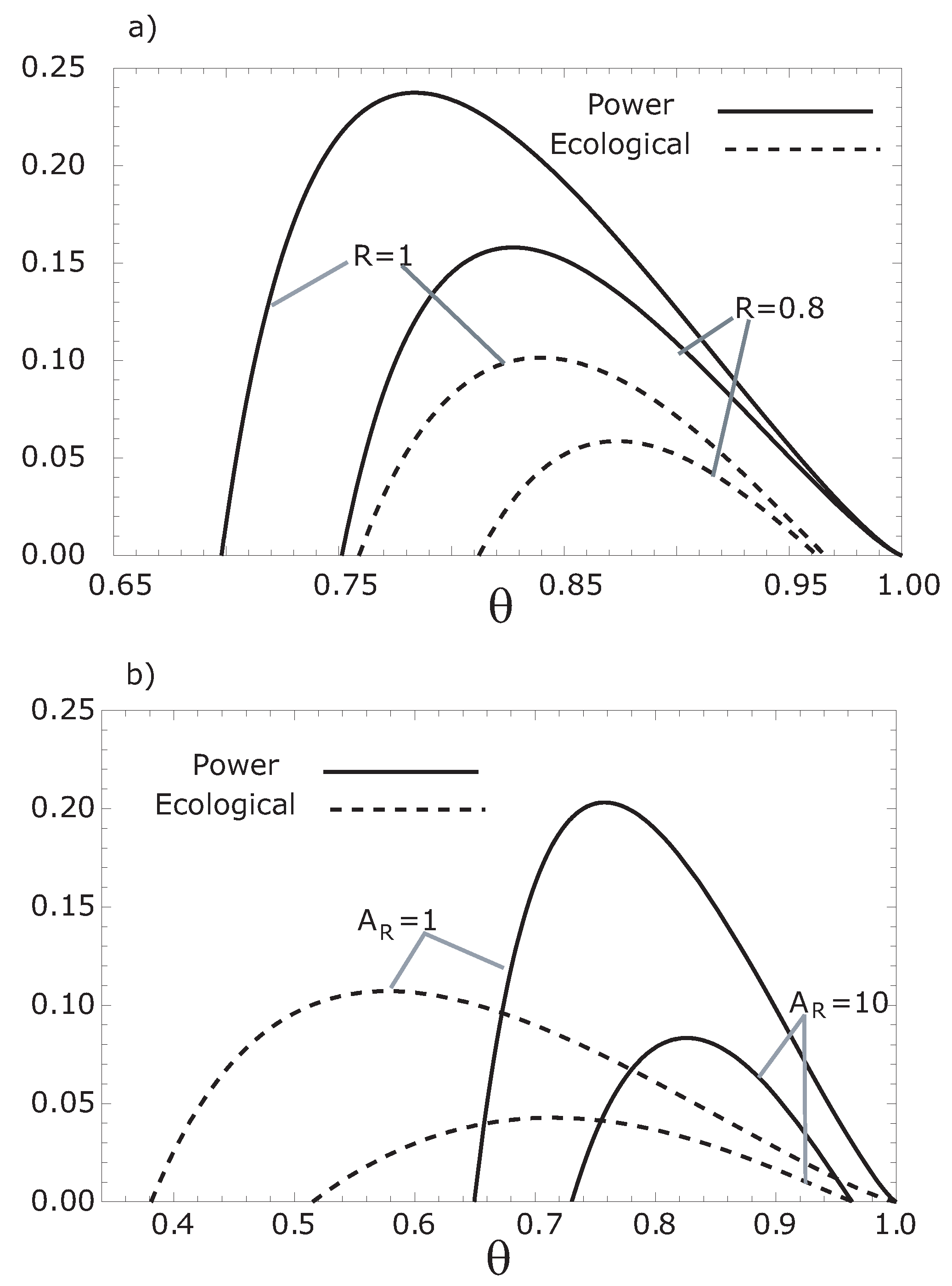
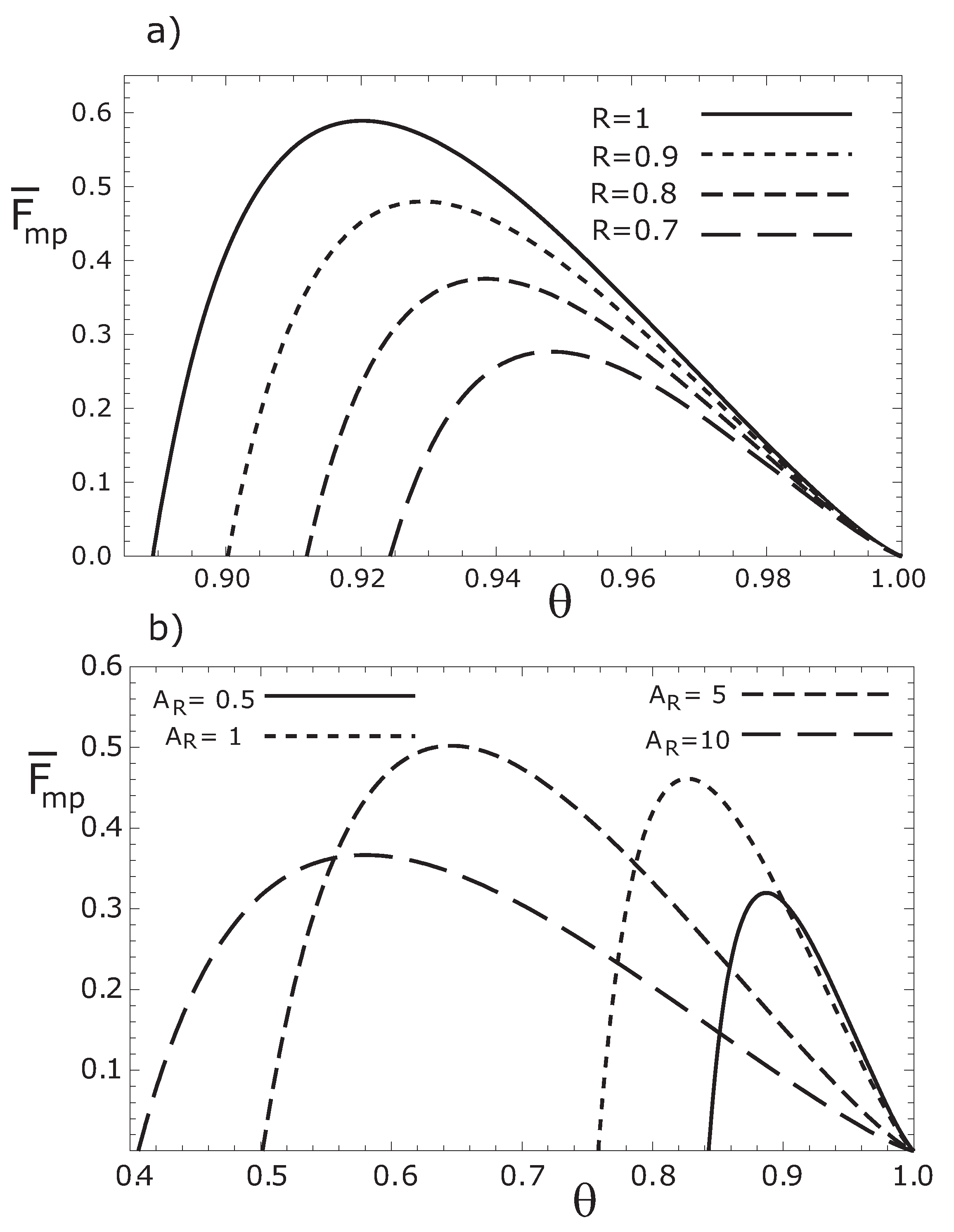
In Figure 2a, we depict the objective function given by Equation (15) versus θ, for several values of the parameter R. In Figure 2b we show the function $F_{mp}$ for several values of the parameter $A_R$.

Figure 2. Variation of the thermoeconomic objective function ${\overline{F}}_{mp}$ respect to $\theta =\frac{T_X}{T_H}$, for (a) different values of the parameter R with $A_R=1$, and for (b) several values of $A_R$ with $R=1$.

Figure 2. Variation of the thermoeconomic objective function ${\overline{F}}_{mp}$ respect to $\theta =\frac{T_X}{T_H}$, for (a) different values of the parameter R with $A_R=1$, and for (b) several values of $A_R$ with $R=1$.

For our thermoeconomic optimization approach, we define another objective function in terms of the so-called ecological function [10,29], divided by the annual investment cost, that is, $F_E=\frac{W-T_L\Sigma }{C_i}$, where Σ is the total entropy production of the engine model. Analogously to Equation (15), the normalized objective function associated to the ecological function is given by,

$$\begin{array}{c}\hfill {\overline{F}}_E=\frac{b{F}_E}{U_L{T}_L}=\frac{1}{1+\frac{A_R(1-f)}{f}}{[(1-\theta )}^{5/4}(\tau +1)-\xi (\tau -1){\left(\frac{\tau -1}{\tau }\right)}^{5/4}-\\ \hfill 2\left[\frac{A_R}{\beta }\left(\frac{T_Y}{T_L}-1\right)\right]-\frac{{(1-\theta )}^{5/4}}{\theta }+\frac{A_R}{\beta }\left(1-\frac{T_L}{T_Y}\right)].\end{array}$$

(17)

And, by using Equations (1–3), the thermal efficiency, η, of the irreversible heat engine can be expressed by,

$$\eta =\frac{\tau \beta {(1-\theta )}^{\frac{5}{4}}-A_R\left(\frac{T_Y}{T_L}-1\right)}{\tau \beta {(1-\theta )}^{\frac{5}{4}}+ϵ\tau {\left(\frac{\tau -1}{\tau }\right)}^{\frac{5}{4}}}.$$

(18)

In Equation (17) we have applied the second law of thermodynamics to calculate the total entropy production given by $\Sigma =\frac{{\dot{Q}}_L}{T_L}-\frac{{\dot{Q}}_H}{T_H}+\frac{Q_H}{T_x}-\frac{Q_L}{T_y}-\frac{Q_{LK}}{T_H}+\frac{Q_{LK}}{T_L}$ (see Figure 1). The dimensionless thermoeconomic objective functions [Equations (15) and (17)], can be plotted with respect to $\theta =T_X/T_H$, for given values of $A_R$ and f as shown in Figure 2a and Figure 2b, and Figure 3a and Figure 3b for the cases of the maximum power output and maximum ecological function conditions, respectively. In all cases we use $\tau =4$, as in [31], where $T_L\approx 300$K and therefore $T_H\approx 1200$K, this value of τ is for comparison with [31], however a more realistic value of $T_H$ could be of the order of 431K [7], which is the effective sky temperature stemming from the dilution of solar energy.

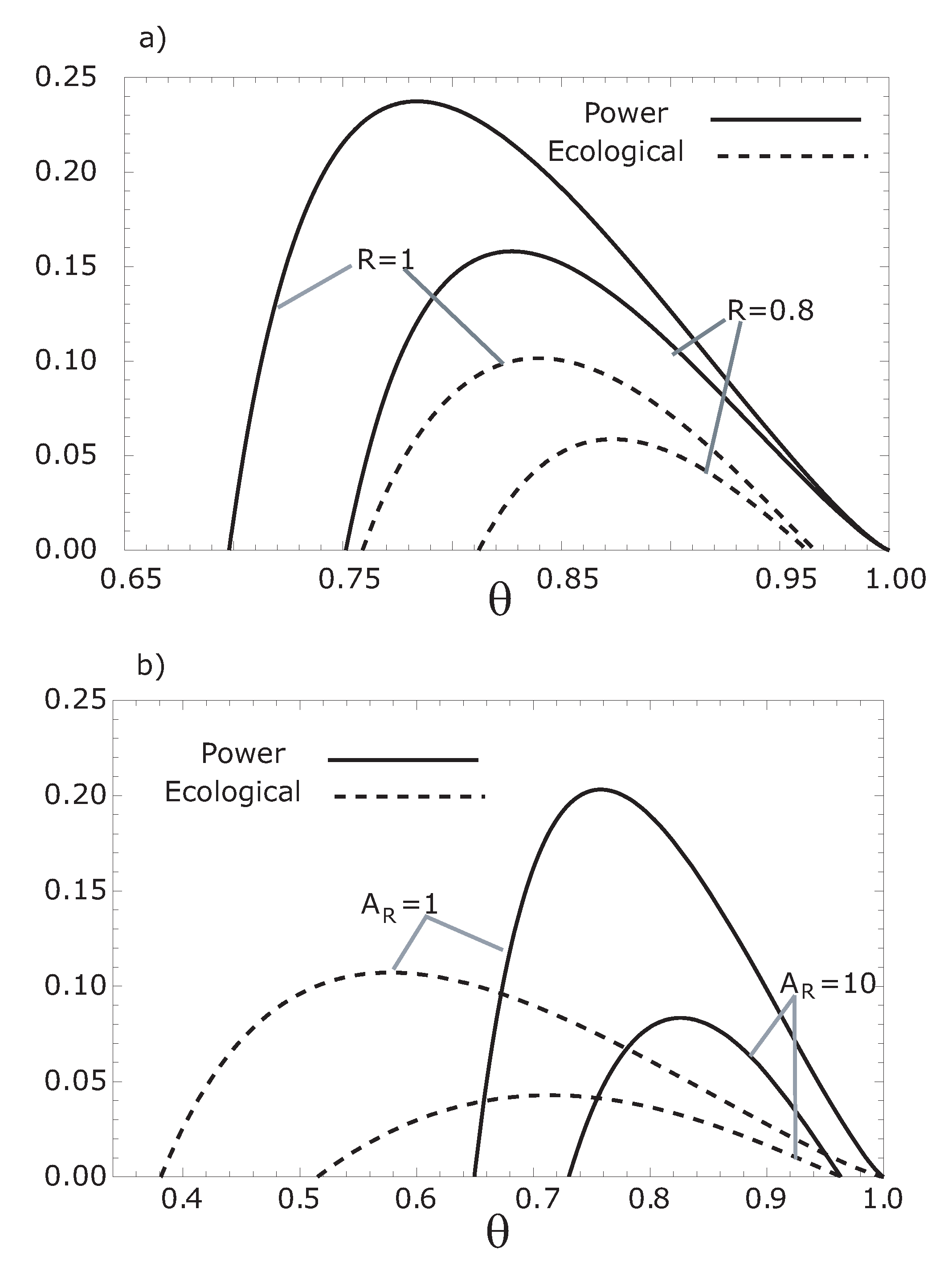
Figure 3. Variation of the thermoeconomic objective function ${\overline{F}}_E$ respect to $\theta =\frac{T_X}{T_H}$, for (a) different values of the parameter R with $A_R=1$, and for (b) several values of $A_R$ with $R=0.8$.

Figure 3. Variation of the thermoeconomic objective function ${\overline{F}}_E$ respect to $\theta =\frac{T_X}{T_H}$, for (a) different values of the parameter R with $A_R=1$, and for (b) several values of $A_R$ with $R=0.8$.

As it could be seen from Figure 2a–Figure 3b, there is a value of θ that maximizes the objective functions for given f, $A_R$ and τ values. In Figure 4, we show the comparison of the aforementioned two objective functions. Since the two objective functions and thermal efficiency depend on the working fluid temperatures $(T_X,T_Y)$, the objective functions given by Equations (15) and (17) can be maximized with respect to $T_X$ or $T_Y$, that is, we calculate $\frac{dF}{d\theta }{|}_{\theta ={\theta }^{*}}=0$, the ${\theta }^{*}$ values obtained give us the maximum values for ${\overline{F}}_{mp}$ and ${\overline{F}}_E$ functions, respectively. This optimization procedure has been numerically carried out in the next section [3,31].

Figure 4. Comparison of both the thermoeconomic objective functions, ${\overline{F}}_{mp}$ and ${\overline{F}}_E$, respect to $\theta =\frac{T_X}{T_H}$, for (a) different values of the parameter R and for (b) several values of $A_R$.

Figure 4. Comparison of both the thermoeconomic objective functions, ${\overline{F}}_{mp}$ and ${\overline{F}}_E$, respect to $\theta =\frac{T_X}{T_H}$, for (a) different values of the parameter R and for (b) several values of $A_R$.

3. Numerical Results and Discussion

We can observe from Figure 2 and Figure 3 that the maximum thermoeconomic objective functions (${\overline{F}}_{mp}$ and ${\overline{F}}_E$) diminish while the corresponding optimum hot working fluid temperatures shift towards $T_H$ when the internal irreversibility parameter R decreases. On the other hand, the thermoeconomic objective function at MER is less than the thermoeconomic objective function at MPR (see Figure 4). 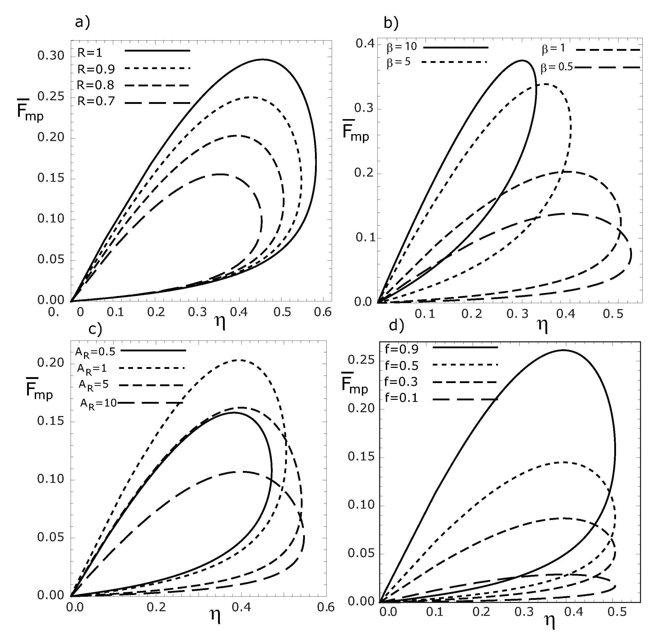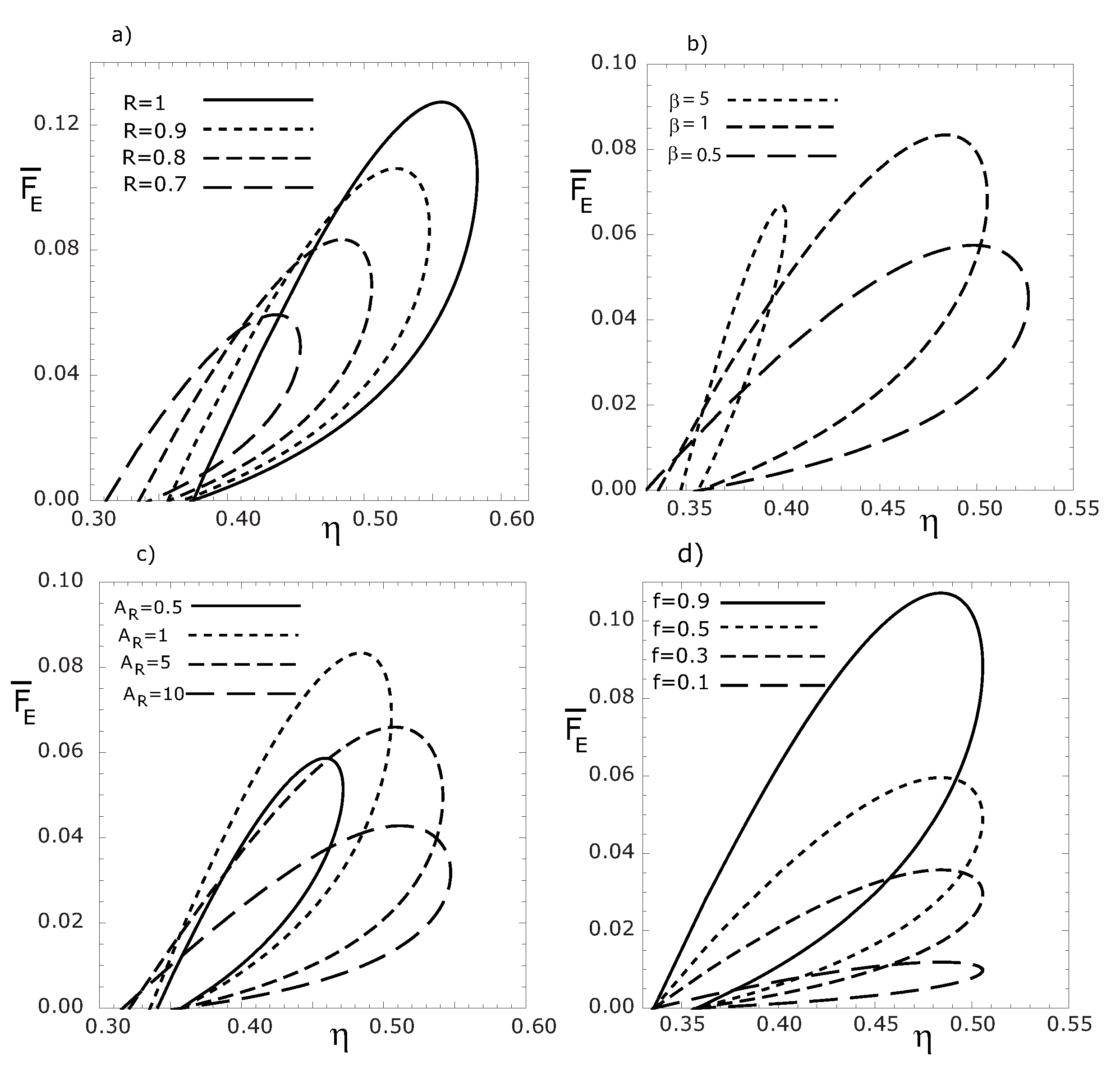In Figure 5 and Figure 6, for both MPR and MER cases, the variation of the dimensionless thermoeconomic objective functions with respect to thermal efficiency for several values of R, β, $A_R$, and f are presented. From Figure 5a–Figure 5d, we see that the loop shaped curves become smaller as f, β and $A_R$ decrease. We can also see that the maximum thermal efficiency is independent of f values, while the maximum ${\overline{F}}_{mp}$ (or ${\overline{F}}_E$), decreases for decreasing f values (see Figure 5d and Figure 6d).

Figure 5. Variations of the dimensionless thermoeconomic objective function ${\overline{F}}_{mp}$, with respect to thermal efficiency for various R (a), β (b), $A_R$ (c) and f (d) values, respectively. ($\xi =0.02$).

Figure 5. Variations of the dimensionless thermoeconomic objective function ${\overline{F}}_{mp}$, with respect to thermal efficiency for various R (a), β (b), $A_R$ (c) and f (d) values, respectively. ($\xi =0.02$).

Figure 6. Variations of the dimensionless thermoeconomic objective function ${\overline{F}}_E$, with respect to thermal efficiency for various R (a), β (b), $A_R$ (c) and f (d) values, respectively. ($\xi =0.02$).

Figure 6. Variations of the dimensionless thermoeconomic objective function ${\overline{F}}_E$, with respect to thermal efficiency for various R (a), β (b), $A_R$ (c) and f (d) values, respectively. ($\xi =0.02$).

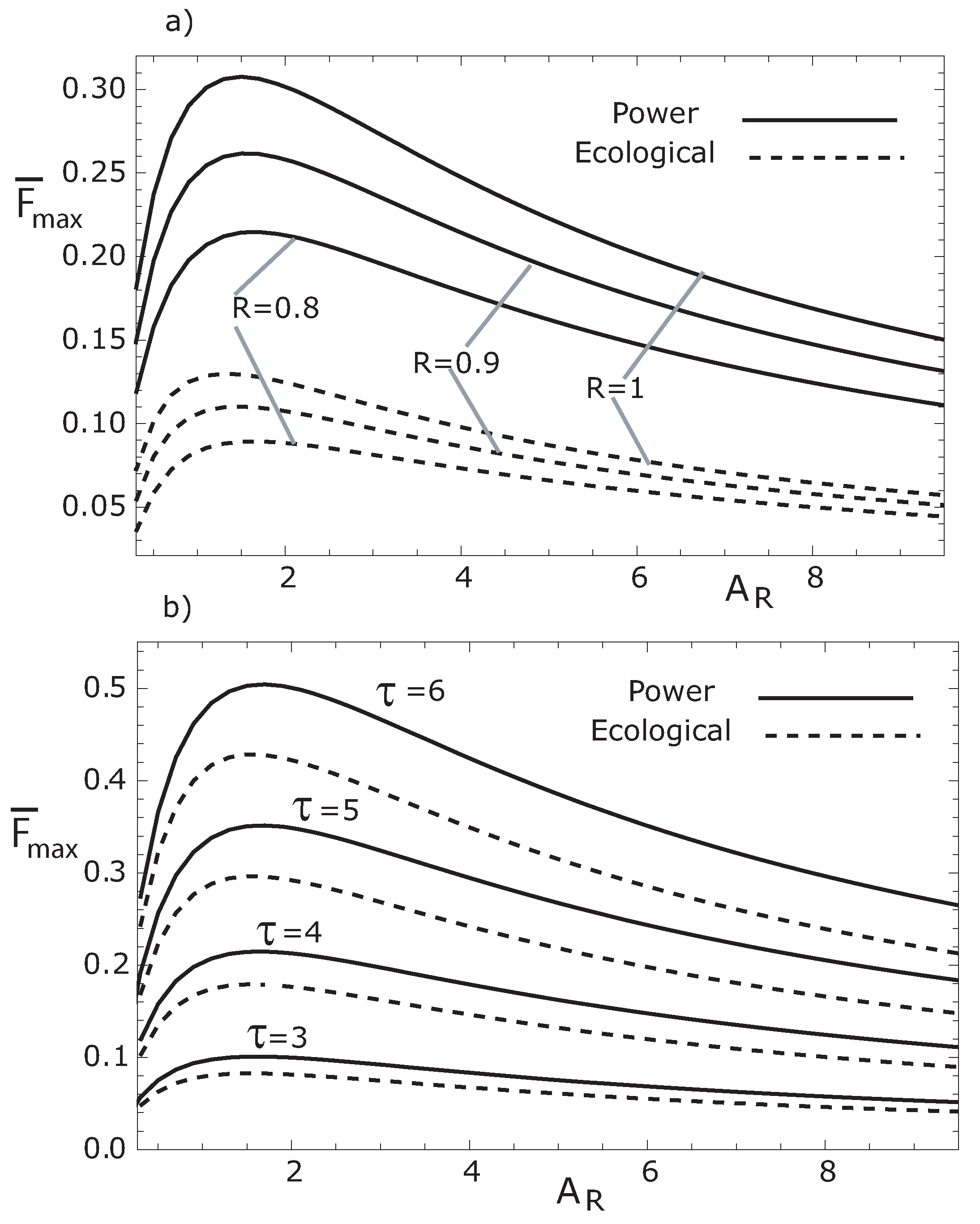
In Figure 7 we show the variation of the maximum dimensionless thermoeconomic objective functions (${\overline{F}}_{max}$, for both MPR and MER cases) with respect to the ratio $A_R=\frac{A_L}{A_H}$ for different values of the parameter R (see Figure 7a) and for several values of the temperature ratio $\tau =\frac{T_H}{T_L}$ (see Figure 7b). We can observe in Figure 7, for both MPR and MER, that as $A_R$ increases, ${\overline{F}}_{max}$ increases to its peak value, and then smoothly decreases. We can also observe that ${\overline{F}}_{max}$ increases and the optimal $A_R$ value considerably decreases for increasing R and τ values.

Figure 7. Variation of the two maximum thermoeconomic objective functions with respect to $A_R$ for: (a) two values of R with $\tau =4$, and (b) for several values of τ with $R=0.8$. In both cases, $\beta =1$, $f=0.7$ and $\xi =0.02$.

Figure 7. Variation of the two maximum thermoeconomic objective functions with respect to $A_R$ for: (a) two values of R with $\tau =4$, and (b) for several values of τ with $R=0.8$. In both cases, $\beta =1$, $f=0.7$ and $\xi =0.02$.

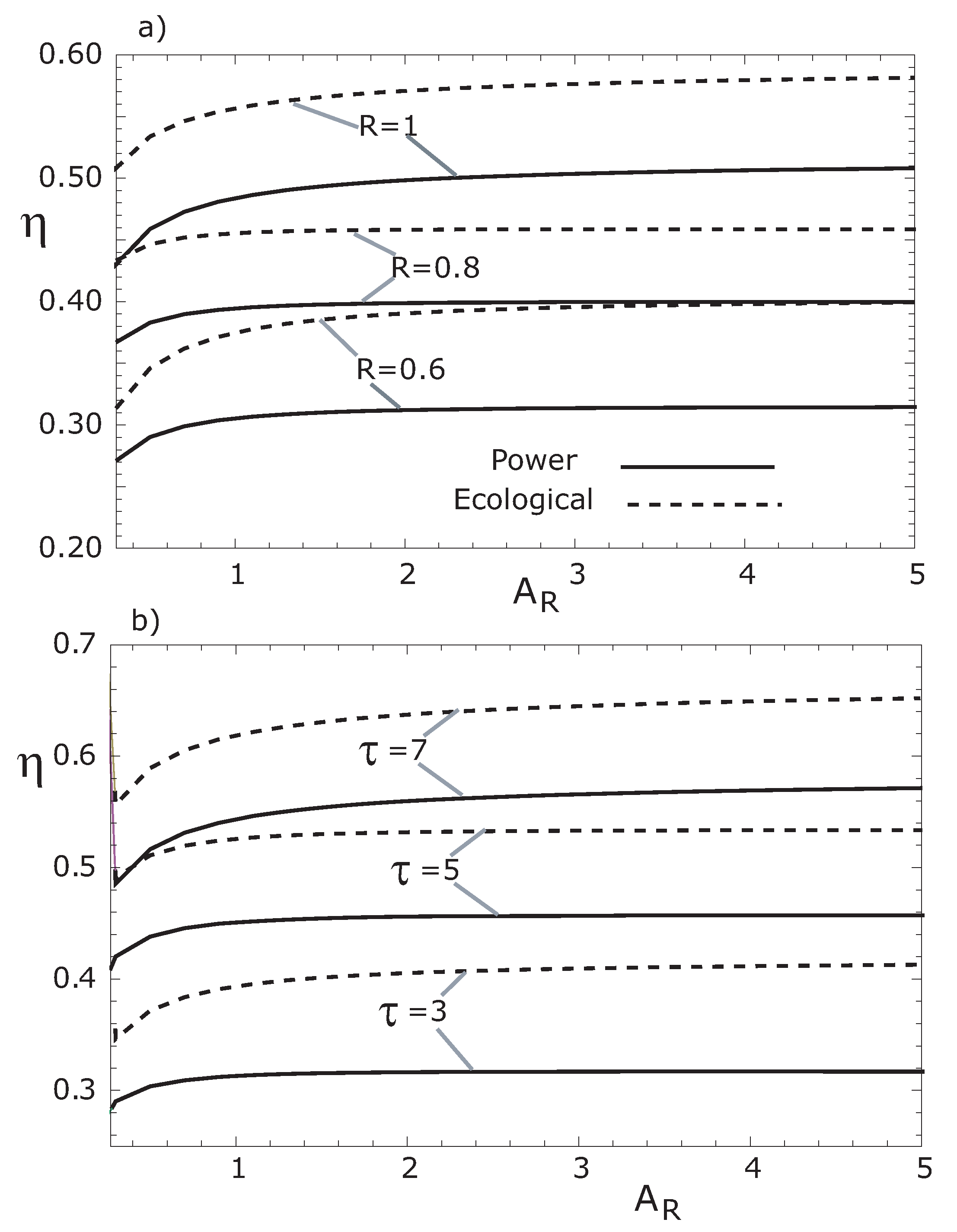
In Figure 8, we show the optimal thermal efficiencies for both MPR and MER cases. In this figure, we can observe that the optimal thermal efficiencies under MER (for all values of the parameter R, see Figure 8a) and for several values of the parameter τ, see Figure 8b) are bigger than the optimal thermal efficiencies at MPR. Besides, these optimal efficiencies satisfy the following inequality:

$${\eta }_C>{\eta }_{opt}^{MER}>{\eta }_{opt}^{MPR}>{\eta }_{CA},$$

(19)

where the subscripts C and $CA$ refer to Carnot and Curzon-Ahlborn respectively. The previous inequality was recently obtained by Barranco-Jiménez et al. for the case of an endoreversible model of a solar driven-heat engine [4].

Figure 8. Optimal thermal efficiencies vs. $A_R$ for the two regimes. (a) For three values of R with $\tau =4$ and (b) For three values of τ with $R=0.8$. In both cases, $\beta =1$, $f=0.7$ and $\xi =0.02$ (these optimal thermal efficiencies were obtained by substituting ${\theta }^{*}$ in Equation (18)).

Figure 8. Optimal thermal efficiencies vs. $A_R$ for the two regimes. (a) For three values of R with $\tau =4$ and (b) For three values of τ with $R=0.8$. In both cases, $\beta =1$, $f=0.7$ and $\xi =0.02$ (these optimal thermal efficiencies were obtained by substituting ${\theta }^{*}$ in Equation (18)).

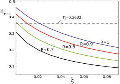
On the other hand, regarding actual photothermal converters, their thermal efficiencies are not easily available in the technical literature. A reported case is that corresponding to the solar power plant Eurelios at Adrano (Italy) [7]. The experimental efficiency for this plant is around 0.13, which is smaller than the theoretical value (around 0.68) given by the De Vos model [7]. For the model of the present work, we can see in Figure 8 that for $\tau =3$ we obtain efficiencies around 0.3, which is bigger than the experimental one, but remarkably smaller than the De Vos value. 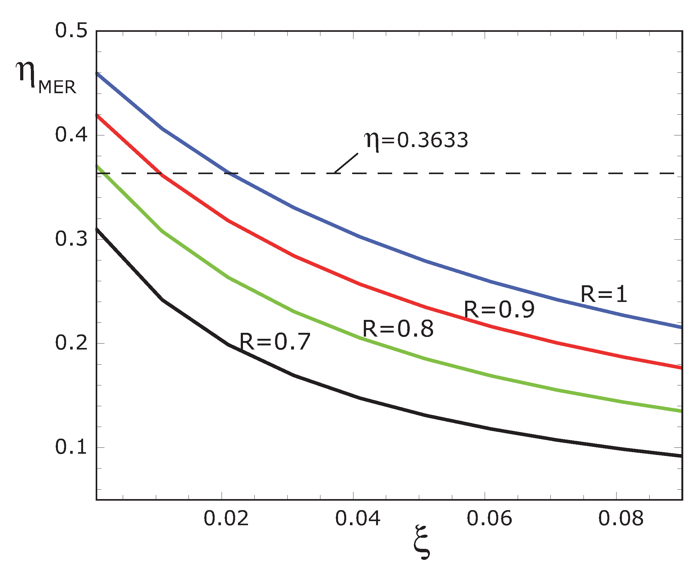If we locate the 0.13 point in Figure 6 (a, b, c or d) it corresponds to a negative ecological function, that is, this plant seemingly has a dissipation larger than its power output. Thus, under the perspective here formulated, some solar power plants have yet a large range of efficiencies to be reached by means of design improvements. As it was asserted by Wu [30], there are few solar engine data to compare with TTF corresponding models. However, Wu took two solar thermal power generation plants given by Hsieh with efficiency values of 0.36 and 0.37, respectively [35]. Wu [30] proposed a simple endoreversible model of the Curzon-Ahlborn type to compare with Hsieh’s data. His numerical comparison is very good and this author concludes that these solar power plants should be operated closer to the CA-efficiency. However, in Figure 9 we show a numerical result corresponding to our model working at maximum ecological regime but with several irreversibilities, which in this case are: $R=0.9$, $\xi =0.11$ and $R=1$, $\xi =0.023$, respectively. As it can be seen, we obtain efficiencies very close to the experimental ones but under some more realistic conditions. Thus, this scenario is also possible to describe the performance regime to the Hsieh’s plants.

Figure 9. Optimal thermal efficiencies vs. ξ at maximum ecological regime, for four values of R with $\tau =2.46$, $A_R=1$ and $\beta =4.1373$ for comparison with the values reported by Wu [30].

Figure 9. Optimal thermal efficiencies vs. ξ at maximum ecological regime, for four values of R with $\tau =2.46$, $A_R=1$ and $\beta =4.1373$ for comparison with the values reported by Wu [30].

4. Conclusions

In this work, a thermoeconomic performance analysis using finite time/finite size thermodynamics has been carried out for an irreversible solar-driven heat engine model in terms of the maximization of two objective functions. The objective functions have been defined as the quotient between power output and the ecological function per unit total investment cost, respectively. By means of the maximization of these objective functions, the optimum thermoeconomic performance and the corresponding best design parameters of the solar-driven heat engine were determined. In this context, the effects of the economic parameter, f, and the ratio of heat transfer areas, $A_R$, on the optimal thermoeconomic performance have been investigated. For the model here studied which uses a Dulong-Petit heat transfer law (convective-conductive plus radiative effects) at the superior thermal coupling (see Figure 1) instead of only the simultaneous conduction and radiation modes as in [27], we systematically obtain lower values for $T_X$ and $A_R$. That is, for a fixed value of $A_H$, our model leads to smaller heat transfer areas for the cold-side heat exchanger. On the other hand, we show how the optimal thermal efficiencies under maximum ecological conditions are bigger than the optimal thermal efficiencies at maximum power conditions. This result has been observed in all kind of thermal engine models operating under maximum ecological conditions. Our model takes into account several irreversibilities, which are not usually considered in solar driven heat-engine models. Additionally, we have presented some numerical comparisons of our results with efficiencies of three actual solar driven power plants.