Wavelet-Based Multi-Scale Entropy Analysis of Complex Rainfall Time Series

Abstract

This paper presents a novel framework to determine the number of resolution levels in the application of a wavelet transformation to a rainfall time series. The rainfall time series are decomposed using the à trous wavelet transform. Then, multi-scale entropy (MSE) analysis that helps to elucidate some hidden characteristics of the original rainfall time series is applied to the decomposed rainfall time series. The analysis shows that the Mann-Kendall (MK) rank correlation test of MSE curves of residuals at various resolution levels could determine the number of resolution levels in the wavelet decomposition. The complexity of rainfall time series at four stations on a multi-scale is compared. The results reveal that the suggested number of resolution levels can be obtained using MSE analysis and MK test. The complexity of rainfall time series at various locations can also be analyzed to provide a reference for water resource planning and application.

1. Introduction

Many new methods and models are available for analyzing and simulating hydrological time series. In practice, studying hydrological time series is difficult because they are affected by complex factors. Each hydrological time series contains several frequency components which are governed by their own factors. Use of only single resolution components to model a hydrological time series does not allow the easy elucidation of the internal mechanism. Wavelet-based multi-resolution analysis must be employed in the modeling of hydrological time series. Wavelet transform and multi-scale entropy can be adopted in analyzing multi-scale time series.

This investigation applies a wavelet transform and MSE to the rainfall time series. Wavelets have been extensively used in the modeling, analysis and forecasting of rainfall time series. The most important feature of a wavelet is its multi-resolution property, which increasingly is being exploited in processing images and signals. Labat [1] has reviewed the wavelet applications in the field of earth science and has illustrated new wavelet analysis methods in the field of hydrology. Partal and Kişi [2] have combined a discrete wavelet transform with neuro-fuzzy systems to forecast precipitation. Their wavelet-neuro-fuzzy model fits observed data very closely, especially when the time series have zero precipitation in the summer months and peaks in the testing period.

Sang et al. [3] have developed a new method of hydrological series data study, main series spectral analysis (MSSA), which is based on two conventional hydrologic series analysis methods: wavelet analysis (WA) and maximum entropy spectral analysis (MESA). MSSA improves the identification of periods by effectively reducing the effect of hydrological noise. Mishra et al. [4] have exploited the concept of entropy to examine the spatial and temporal variability of precipitation time series for the state of Texas, USA. In their study, marginal entropy has been employed to elucidate the variability associated with monthly, seasonal, and annual time series. They have also used apportionment entropy to study the intra-annual and decadal distributions of monthly and annual precipitation, and used intensity entropy to study the numbers of rainy days in a year and decade. Brunsell [5] has utilized information theory metrics to determine the spatial and temporal variability of daily precipitation over the continental US. Entropy is determined from the daily precipitation records and the distribution of sizes of precipitation events. Relative entropy is also computed from the two records and the Hurst exponent is calculated for comparison. Wavelet multi-resolution analysis and relative entropy are applied to identify the breakpoint, which the Hurst exponent cannot be used to resolve.

MSE analysis is usually applied to the analysis of multi-scale time series. Entropy is commonly used to characterize the complexity of a signal. Kolmogorov-Sinai (KS) entropy can be used to represent complexity and is computed from the average production rate of new information. KS entropy is the basis of approximate entropy. Approximate entropy is effective for analyzing the complexity of short time series. Richman and Moorman [6] have defined the sample entropy which is a modification of approximate entropy. Both KS entropy and approximate entropy determined use a single scale. They neglect the characteristics when the number of scales exceeds one. Costa et al. [7] have defined and applied MSE, which is based on sample entropy and is effective in analyzing the complexity of physiological signals. Their results have demonstrated that MSE curve identified diseased hearts to have a significant decrease in the sample entropy on multiple time scales, indicating a lower degree of complexity.

The number of resolution levels to be used in the application of a wavelet transform to a rainfall time series should be determined. The smoothing of the detailed signals and the residual improve as the number of resolution levels increases. However, greater resolution level takes more models for modeling and leads to error propagation. The error, i.e., the difference between the estimation and observations, increases with the number of resolution levels. This investigation proposes a new framework for determining the number of resolution levels required in the application of a wavelet transform to rainfall time series analysis. The number of resolution levels can be determined by MSE analysis and MK test. The central concept of this study is that an original rainfall time series can be decomposed into residuals and detailed signals using redundant wavelet transforms. Then, MSE analysis and MK test is applied to the decomposed rainfall time series.

The following sections define the redundant wavelet transform, describe the structure of the MSE, present a case study of four rainfall stations in Taiwan to demonstrate the effectiveness of the presented method, and, discuss the results to draw the conclusions.

2. Wavelet Transform

2.1. Introduction of Wavelet Transform

The continuous wavelet transform of a continuous function outputs a continuum of scales. However, the input data are generally discretely sampled, and may be in the form of hydrological time series. The discrete wavelet transform (DWT) of a vector is the outcome of a linear transformation that yields a new vector whose dimensions are equal to those of the primeval vector. This transformation is also called decomposition and can be performed efficiently using Mallat’s MRA algorithm [8].

Nevertheless, the orthonormal DWT requires that the input data have a number of values which is an integer power of two. The number of resolution levels is naturally limited by log₂ of the number of values in the input. This limitation is inappropriate for a hydrological time series, especially during the short duration of typhoon events in Taiwan.

Aussem and Murtagh [9] have introduced the “à trous” wavelet decomposition. The fundamental idea that underlies MRA or multi-scale analysis is the application of a wavelet transform to decompose signals into different resolution levels or scales. The signal, which decomposes into coarse resolution level, is either an approximation signal or a smooth trend. The signal decomposes into fine resolution level, and is called a detailed signal. The wavelet transform can be considered as a bridge among signals at various resolution levels. In contrast, the input data of the à trous wavelet transform may take any values, such that the number of resolution levels is unlimited. Not only is this à trous wavelet transform parsimonious but the filter outputs can also be meaningfully interpreted [9]. The calculation of the wavelets is trivially performed in a cascaded scheme, and involves an appealing reconstruction formula that will be exploited.

Other advantages of the à trous wavelet transform are as follows [10]: (1) The evolution of the wavelet decomposition can be followed from level to level; (2) The algorithm generates a single wavelet coefficient series at each level of the decomposition; (3) The wavelet coefficients are computed for each location, facilitating the detection of a dominant feature; (4) The algorithm is easily implemented. Additionally, the recursive computation of this algorithm is very effective and can be achieved using filter banks [11].

2.2. Redundant Wavelet Transform

The à trous algorithm is a redundant wavelet transform [10,11,12]. The wavelet transform decomposes the input hydrological time series into detailed signals and a residual (or an approximation) so the original hydrological time series is expressed as an additive combination of wavelet coefficients at various resolution levels. The procedure for decomposing the discrete hydrological time series $s(k)$ is to perform successive convolutions using a discrete low-pass filter c [9]:

$$s_{i+1}(k)={\displaystyle \sum _{l=-\infty }^{\infty }c(l)}{s}_i(k+2^{i}l)$$

(1)

where $s_i$ denotes the approximation signal at revolution level i. The finest scale is used to specify the original hydrological time series x(k), i.e., $s_0$(k) = x(k). The increase in distances between the sampled points ($2^{i}l$) explains the application of the name “à trous” to this method [9]. A $B_3$ spline, defined as (1/16, 1/4, 3/8, 1/4, 1/16), is generally used in a low-pass filter c [9,11], to fulfill the compact support condition (required for a wavelet transform), and to be point-symmetric. Wavelet coefficients $w_i$ are obtained from determining the differences among successive smoothed versions of the signal, as shown below [9]:

$$w_i(k)=s_{i-1}(k)-s_i(k)$$

(2)

Wavelet coefficients provide the “detailed” signal, which in practice can be used to capture the tiny but meaningful characteristics in the data. Such a characterization can cause information loss if the original data vector cannot be reconstructed from the wavelet components. In addition, the “residual” terms $s_p$, representing the “background” data, are added to the wavelet coefficients. The set $\Re =\{w_1,w_2,\dots ,w_p,s_p\}$ represents the wavelet transform of the data, i.e., wavelet coefficients, up to a resolution level of p. Aussem and Murtagh [9] have presented the wavelet expansion of time series, in terms of wavelet coefficients:

$$x(k)=s_p(k)+{\displaystyle \sum _{i=1}^p{w}_i(k)}$$

(3)

3. Multi-Scale Entropy Analysis

3.1. Sample Entropy

Richman and Moorman [6] defined the so-call sample entropy which provides a measure of an “orderly structure” in a time series by testing if there are any repeated patterns of various lengths. The sample entropy is the exact value of the negative average natural log of the conditional probability. Suppose that the data length of the original time series $x\text{(1), }x\text{(2),}\mathrm{...}\text{, }x\text{(}N\text{)}$ is N; the sample entropy of the time series is calculated below [6,13].

(I) The m-dimensional vector, $X\text{(}i\text{)}=\left[x\text{(}i\text{), }x\text{(}i+\text{1),}\mathrm{...}\text{, }x\text{(}i+m\text{-1)}\right]$, comprises a time series, where i = 1,2,…,N – m + 1.

(II) Define the distance $d\left[X\text{(}i\text{), }X\text{(}j\text{)}\right]$ between X(i) and X(j) as follows.

$$d\left[X\text{(}i\text{), }X\text{(}j\text{)}\right]=\text{max}\left[\left|x\text{(}i+k\text{)-}x\text{(}j+k\text{)}\right|\right]$$

(4)

where k = 0,1,2,…, m − 1. Calculate the distance $d\left[X\text{(}i\text{), }X\text{(}j\text{)}\right]$ between X(i) and other vector X(j), where j= 1,2,…,N – m + 1, but j ≠ i.

(III) Count the $d\left[X\text{(}i\text{), }X\text{(}j\text{)}\right]$ that are less small than a given threshold r. Then compute the ratio of this number to the total number N − m, as follows:

$${\text{C}}_i^m\text{(}r\text{)}=\left\{\text{the number of }d\right[X\text{(}i\text{), }X\text{(}j\text{)}]<r\}\text{ / (}N-m\text{, }i=\text{1,2,…,}N–m+1.$$

(5)

(IV) Find the average ${\text{C}}_i^m\text{(}r\text{)}$ for all i, as follows:

$${\text{C}}^m\text{(}r\text{)}=\frac{{\displaystyle \sum {\text{C}}_i^m\text{(}r\text{)}}}{N\text{-}m+1}\text{, i = 1,2,…,}N–m+1.$$

(6)

(V) Add one to the number of dimensions of the vector, yielding m + 1 dimensions. Repeat step (I) to step (IV), yielding ${\text{C}}^{m+\text{1}}\text{(}r\text{)}$.

(VI) The theoretical sample entropy of the time series is given by:

$$\text{SampEn (}m\text{,}r\text{,}N\text{)}=\text{-ln}\left[{\text{C}}^{m+\text{1}}\text{(}r{\text{)/C}}^m\text{(}r\text{)}\right]$$

(7)

3.2. Multi-Scale Entropy

The parameters of sample entropy are determined by a single differentiation. The sample entropy, which is used in the analysis of a single scale factor, does not include the characteristics of the time series when the number of scale factor exceeds one. Costa et al. [7] developed a multi-scale entropy analysis building upon the definition of the so call sample entropy proposed by Richman and Moorman [6]. Suppose that $x\text{(1), }x\text{(2),}\mathrm{...}\text{, }x\text{(}N\text{)}$ is the original time series. The time series at various scale factors, {$y^{\text{(}\tau \text{)}}$}, could be obtained using the following procedure [7,13]:

(I) Let $y_j^{\text{(}\tau \text{)}}=\frac{{\displaystyle \sum x\text{(}i\text{)}}}{\tau }$, where $i=\text{(}j\text{ -1)}\tau +\text{1,}\mathrm{...}\text{,}j\tau$, j = 1,2,…,N/τ. The data length of the time series equals that of the original time series divided by the scale factor τ.

(II) Compute the sample entropy {$y^{\text{(}\tau \text{)}}$} for all scale factors τ.

The above procedure, called multi-scale entropy analysis, is used to analyze entropy when the scale factor exceeds one. When τ = 1, {$y^{\text{(}\tau \text{)}}$} equals the original time series.

4. Application and Analysis

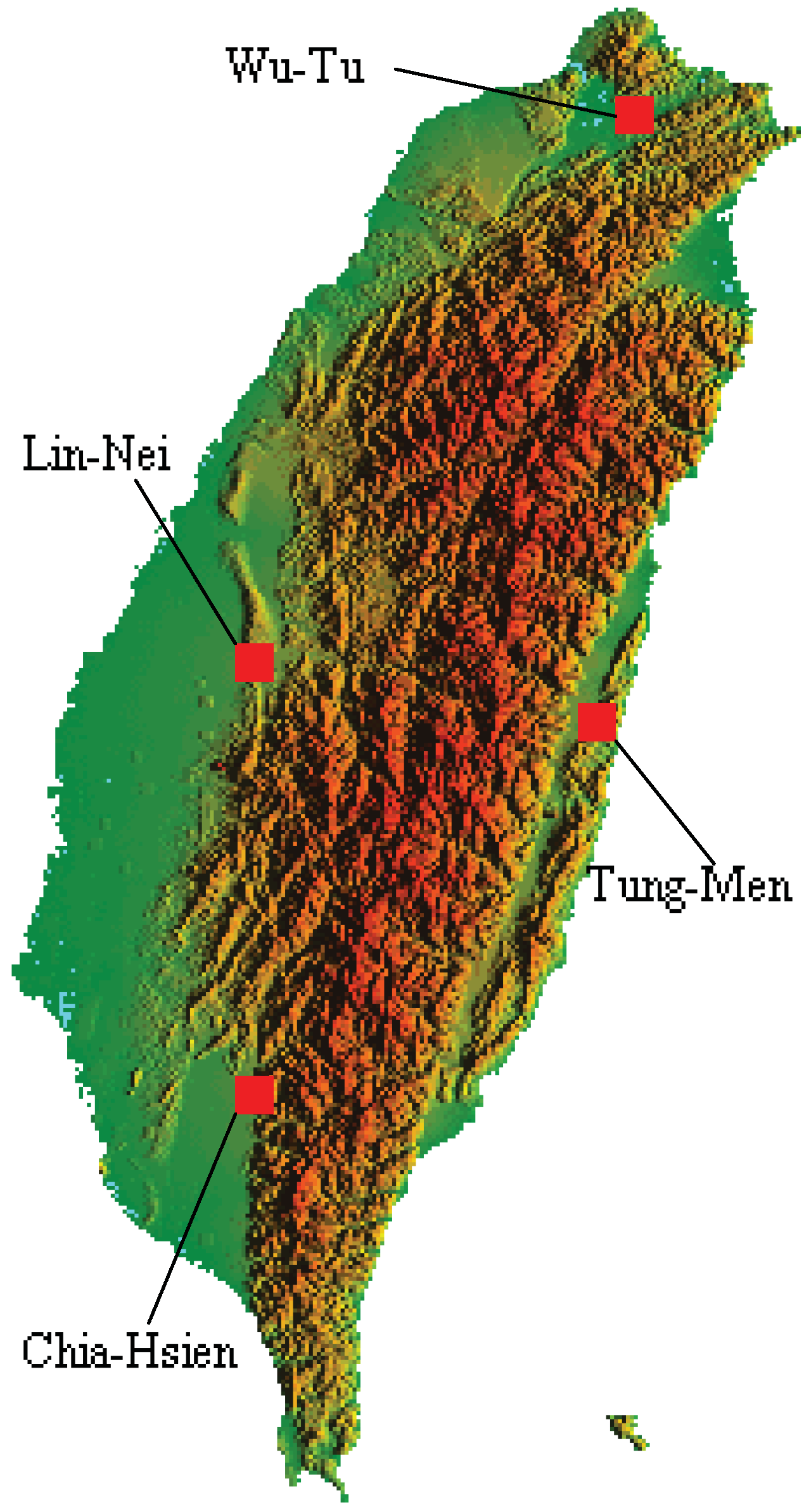
This investigation involves the Wu-Tu (No. 01B030), Lin-Nei (No. 01J930), Chia-Hsien (No. 01P660), and Tung-Men (No. 01T070) rainfall stations, located in northern, middle, southern, and eastern Taiwan, respectively, as shown in Figure 1. The monthly rainfall data from these four rainfall stations from 1963 to 2000 are used in the case study. The series average was subtracted from the monthly rainfall time series.

The à trous redundant wavelet transform has been applied to the four monthly rainfall time series. The number of resolution levels has been set to five in advance. The original rainfall time series have been decomposed into the residuals and wavelet coefficients. The MSE analysis has then been applied to the above residuals to extract some of the hidden characteristics of the original rainfall time series.

To quantitatively determine the suggested resolution level and test the robustness of proposed method, the MK test [14] is applied to MSE curve. The graph of sample entropy as a function of τ is referred to as the MSE curve, which can be interpreted as a measure of information content on multiple time series [15]. MK test is suitable to detect the obvious trend in a series using the order of data. Assume that there are N samples, X(i) ($i=1,\cdots ,N$), the standard normal variate T is defined as [14]:

$$T=\frac{r^{*}}{\sqrt{{{\sigma }^2}_{r^{*}}}}, r^{*}=\left[\frac{4p}{\left\{N\left(N-1\right)\right\}}\right]-1\mathrm{and} {{\sigma }^2}_{r^{*}}=\frac{2(2N+5)}{\left[9N(N-1)\right]}.$$

(8)

where p is the number of times in all pairs of observations when X(i) is less than X(j) for i < j.

Figure 1. The locations of the four rainfall stations [16].

Figure 1. The locations of the four rainfall stations [16].

The trend of the series is significant at the threshold $T_{\alpha /2}$ if $\left|T\right|>T_{\alpha /2}$. An increasing trend is significant when T is positive and a decrease trend is significant when T is negative. For the standard significance level at $\alpha$ = 0.05 the threshold is $T_{0.05/2}$ = 1.96. In this study, when entropy measure of the residual at M-level increases with scale factor (i.e., $T>T_{0.05/2}$), a statistically significant increase trend (or complexity) exists and the M-level decomposition is not suggested to carry out.

5. Results and Discussion

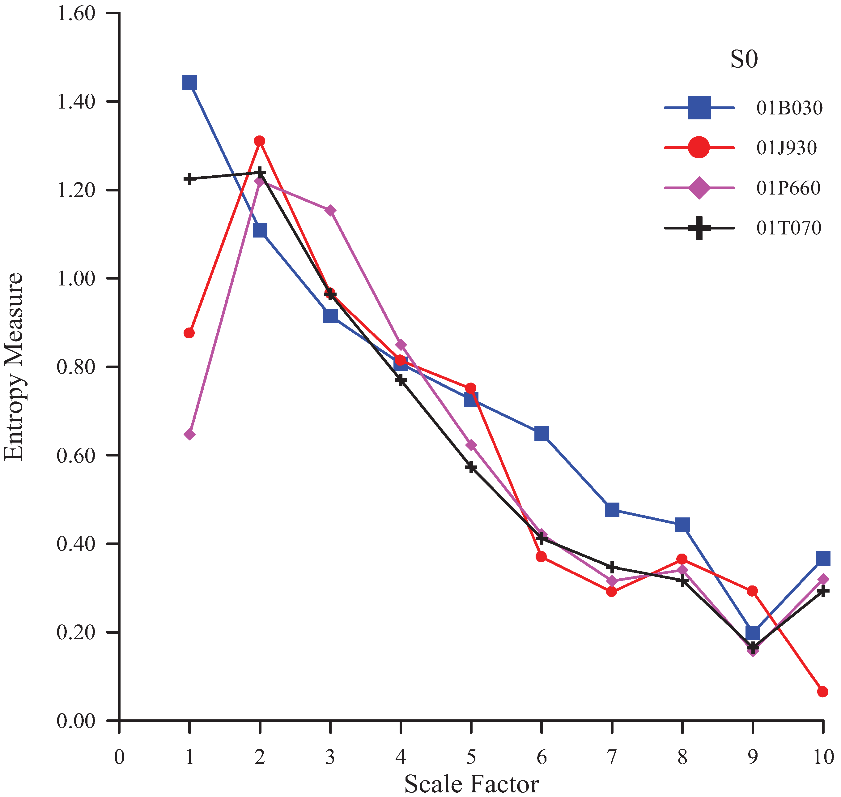
The MSE curves of the original rainfall time series at the four stations have been obtained (Figure 2). The scale factor τ, the number of dimensions m and threshold r are 10, 2 and 0.15 SD (Standard Deviation), respectively [13]. To quantitatively compare the rainfall characteristics among the regions, the MSE analyses for the four stations have been obtained (Table 1). Table 1 demonstrates that the average measured entropy of S0 at the Wu-Tu station (No. 01B030) exceeds those at other stations. Higher entropy corresponds to greater uncertainty. The results show that the rainfall time series at the Wu-Tu station have the most complex structure.

Figure 2. The MSE curves of the original signal (S0) at various stations.

Figure 2. The MSE curves of the original signal (S0) at various stations.

Table 1. The entropy measures of the original signal (S0) at various scale factors for four stations.

Scale Factor	01B030	01J930	01P660	01T070
1	1.44280	0.87499	0.64722	1.22523
2	1.10868	1.30938	1.21979	1.23958
3	0.91505	0.96548	1.15350	0.96414
4	0.80653	0.81377	0.85012	0.76989
5	0.72637	0.75014	0.62295	0.57343
6	0.64986	0.36981	0.42154	0.41224
7	0.47673	0.29079	0.31590	0.34716
8	0.44270	0.36412	0.34077	0.31724
9	0.19843	0.29225	0.15761	0.16510
10	0.36687	0.06402	0.31995	0.29353
Average	0.71340	0.60948	0.60494	0.63075

Table 1. The entropy measures of the original signal (S0) at various scale factors for four stations.

Scale Factor	01B030	01J930	01P660	01T070
1	1.44280	0.87499	0.64722	1.22523
2	1.10868	1.30938	1.21979	1.23958
3	0.91505	0.96548	1.15350	0.96414
4	0.80653	0.81377	0.85012	0.76989
5	0.72637	0.75014	0.62295	0.57343
6	0.64986	0.36981	0.42154	0.41224
7	0.47673	0.29079	0.31590	0.34716
8	0.44270	0.36412	0.34077	0.31724
9	0.19843	0.29225	0.15761	0.16510
10	0.36687	0.06402	0.31995	0.29353
Average	0.71340	0.60948	0.60494	0.63075

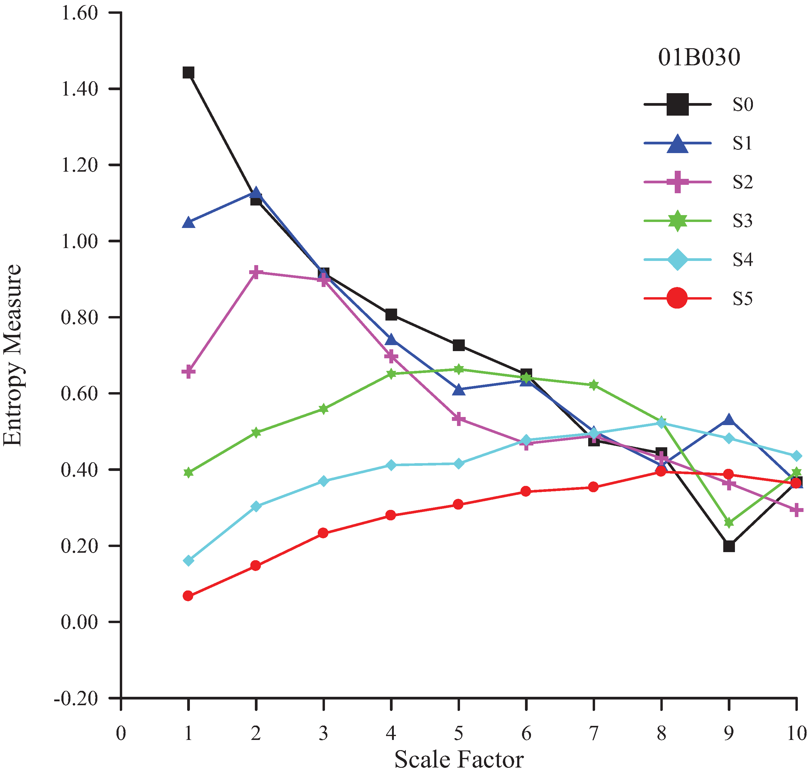
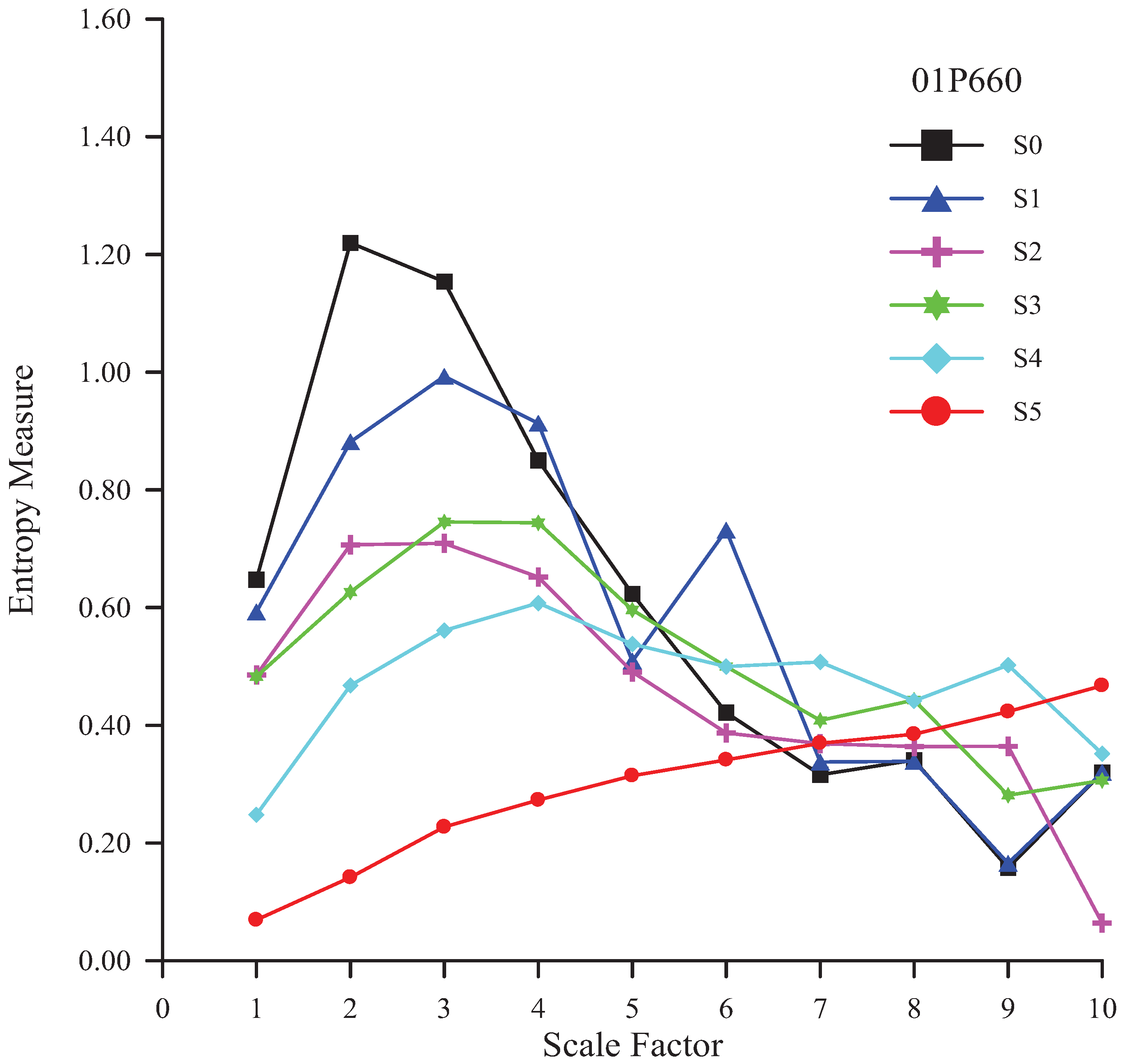
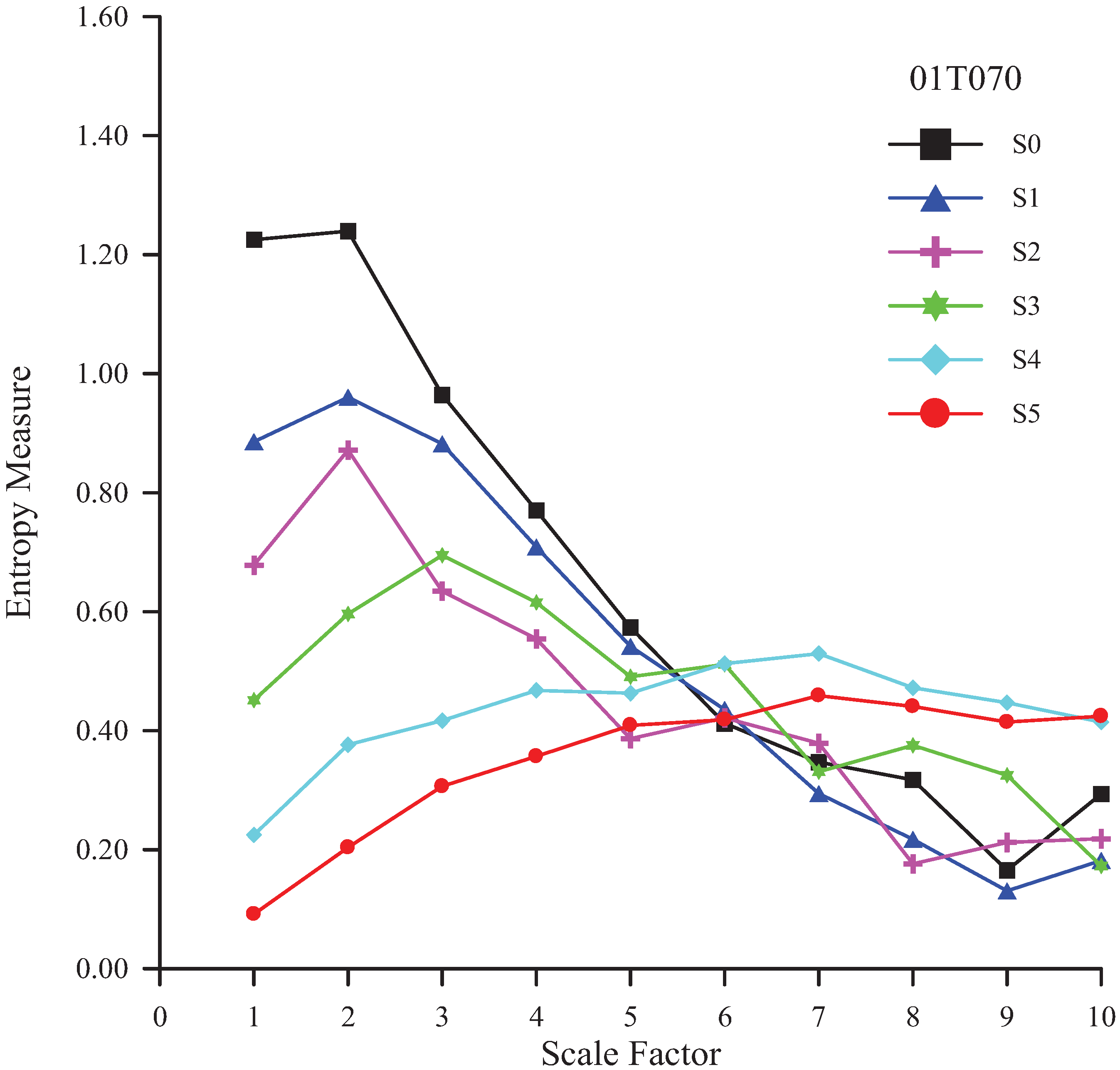
The original time series can be decomposed into the residual S1 and the wavelet coefficient W1. The residual S1 can be decomposed again. The suggested number of resolution levels for a wavelet transform to a rainfall time series should be determined. An MSE analysis of the residuals at various resolution levels (from 1 to 5) for each station is conducted to determine the number of resolution levels. The scale factor, the number of dimensions, and threshold are 10, 2, and 0.15 SD, respectively [13]. S0 denotes the original rainfall time series. S1, S2, S3, S4 and S5 represent the residual with one, two, three, four, and five resolution levels, respectively. The MSE curves of various residuals for the four rainfall stations are shown in Figure 3, Figure 4, Figure 5 and Figure 6.

Figure 3. MSE analysis of various residuals of rainfall time series at the Wu-Tu station.

Figure 3. MSE analysis of various residuals of rainfall time series at the Wu-Tu station.

Figure 4. MSE analysis of various residuals of rainfall time series at the Lin-Nei station.

Figure 4. MSE analysis of various residuals of rainfall time series at the Lin-Nei station.

Figure 5. MSE analysis of various residuals of rainfall time series at the Chia-Hsien station.

Figure 5. MSE analysis of various residuals of rainfall time series at the Chia-Hsien station.

Figure 6. MSE analysis of various residuals of rainfall time series at the Tung-Men station.

Figure 6. MSE analysis of various residuals of rainfall time series at the Tung-Men station.

The number of resolution levels should be determined when applying a wavelet transform to the hydrological time series modeling or rainfall-runoff processes. The smoothing of the detailed signals and the residual improve as the number of resolution levels increases. However, a greater resolution level takes more models for modeling and leads to the error propagation. The error, i.e., the difference between the estimation and observations, increases with the number of resolution levels. Therefore, the number of resolution levels used in the wavelet decomposition need to be accurate. Table 2 shows the standard normal variate of different MSE curves at the four stations. When entropy measure of the residual at M-level increases with scale factor (i.e., $T>T_{0.05/2}$) the M-level decomposition does not carry out. The suggested resolution levels for the four rainfall stations are shown in the last column of Table 2.

Table 2. The standard normal variate of different MSE curves for four stations (m = 2 and r = 0.15SD).

	S0	S1	S2	S3	S4	S5	Suggested Level
01B030	−3.846	−3.309	−3.309	−0.447	2.952	3.488	3
01J930	−3.309	−2.773	−2.952	−1.699	2.952	4.025	3
01P660	−2.952	−2.415	−2.952	−2.415	−0.626	4.025	4
01T070	−3.667	−3.667	−3.130	−2.415	1.342	2.952	4

Table 2. The standard normal variate of different MSE curves for four stations (m = 2 and r = 0.15SD).

	S0	S1	S2	S3	S4	S5	Suggested Level
01B030	−3.846	−3.309	−3.309	−0.447	2.952	3.488	3
01J930	−3.309	−2.773	−2.952	−1.699	2.952	4.025	3
01P660	−2.952	−2.415	−2.952	−2.415	−0.626	4.025	4
01T070	−3.667	−3.667	−3.130	−2.415	1.342	2.952	4

To test the robustness of MSE results, the same analyses have also been performed via removing 25% of the time series (Table 3). The results for Wu-Tu (No. 01B030), Lin-Nei (No. 01J930), and Chia-Hsien (No. 01P660) rainfall stations have not changed. Only the suggested level for Tung-Men (No. 01T070) rainfall station has changed slightly to be 3.

Table 3. The standard normal variate of different MSE curves at four stations when removing 25% of the time series.

	S0	S1	S2	S3	S4	S5	Suggested Level
01B030	−3.488	−3.667	−3.130	−2.057	3.130	3.130	3
01J930	−3.130	−3.309	−2.773	−1.521	3.488	4.025	3
01P660	−2.773	−2.594	−2.773	−2.415	0.626	2.594	4
01T070	−3.667	−3.130	−3.667	−2.415	2.594	2.236	3

Table 3. The standard normal variate of different MSE curves at four stations when removing 25% of the time series.

	S0	S1	S2	S3	S4	S5	Suggested Level
01B030	−3.488	−3.667	−3.130	−2.057	3.130	3.130	3
01J930	−3.130	−3.309	−2.773	−1.521	3.488	4.025	3
01P660	−2.773	−2.594	−2.773	−2.415	0.626	2.594	4
01T070	−3.667	−3.130	−3.667	−2.415	2.594	2.236	3

To illustrate the influence of the sampling rate on MSE results, the same analyses have also been repeated with bi-monthly data (Table 4). The results for all four rainfall stations have not changed.

Table 4. The standard normal variate of different MSE curves at four stations with bi-monthly data.

	S0	S1	S2	S3	S4	S5	Suggested Level
01B030	−3.488	−3.488	−2.415	0.268	3.667	3.846	3
01J930	−1.163	−1.342	0.089	0.805	2.594	4.025	3
01P660	−0.268	−0.089	0.805	0.447	1.521	3.846	4
01T070	−2.952	−2.415	−1.699	−1.878	1.699	4.025	4

Table 4. The standard normal variate of different MSE curves at four stations with bi-monthly data.

	S0	S1	S2	S3	S4	S5	Suggested Level
01B030	−3.488	−3.488	−2.415	0.268	3.667	3.846	3
01J930	−1.163	−1.342	0.089	0.805	2.594	4.025	3
01P660	−0.268	−0.089	0.805	0.447	1.521	3.846	4
01T070	−2.952	−2.415	−1.699	−1.878	1.699	4.025	4

To test the robustness of MSE results, the same analyses have also been performed for r = 0.20SD (Table 5). However, while the overall MSE values shows the expected increase with increasing r, the results for Wu-Tu (No. 01B030) and Lin-Nei (No. 01J930) rainfall stations have not changed. The suggested level for Chia-Hsien (No. 01P660) and Tung-Men (No. 01T070) rainfall stations have changed slightly to be 3.

Table 5. The standard normal variate of different MSE curves at the four stations (m = 2 and r = 0.20SD).

	S0	S1	S2	S3	S4	S5	Suggested Level
01B030	−3.846	−3.130	−2.057	0.805	3.309	3.846	3
01J930	−2.952	−2.594	−0.805	0.089	4.025	4.025	3
01P660	−2.594	−2.236	−1.878	−1.342	2.594	3.846	3
01T070	−3.488	−3.309	−2.952	−0.626	2.594	3.846	3

Table 5. The standard normal variate of different MSE curves at the four stations (m = 2 and r = 0.20SD).

	S0	S1	S2	S3	S4	S5	Suggested Level
01B030	−3.846	−3.130	−2.057	0.805	3.309	3.846	3
01J930	−2.952	−2.594	−0.805	0.089	4.025	4.025	3
01P660	−2.594	−2.236	−1.878	−1.342	2.594	3.846	3
01T070	−3.488	−3.309	−2.952	−0.626	2.594	3.846	3

The same analyses have also been performed for m = 3 and r = 0.25SD (Table 6), with no change of results at all four rainfall stations. In this study, the MSE values with m = 2 and r = 0.15SD can be used to robustly determine the suggested number of resolution levels.

Table 6. The standard normal variate of different MSE curves at the four stations (m = 3 and r = 0.25SD).

	S0	S1	S2	S3	S4	S5	Suggested Level
01B030	−3.667	−2.415	−3.309	−0.626	3.488	3.667	3
01J930	−2.952	−2.952	−2.952	−1.699	4.025	4.025	3
01P660	−3.130	−2.773	−2.594	−2.594	1.699	3.846	4
01T070	−2.952	−3.488	−3.309	−2.236	0.984	4.025	4

Table 6. The standard normal variate of different MSE curves at the four stations (m = 3 and r = 0.25SD).

	S0	S1	S2	S3	S4	S5	Suggested Level
01B030	−3.667	−2.415	−3.309	−0.626	3.488	3.667	3
01J930	−2.952	−2.952	−2.952	−1.699	4.025	4.025	3
01P660	−3.130	−2.773	−2.594	−2.594	1.699	3.846	4
01T070	−2.952	−3.488	−3.309	−2.236	0.984	4.025	4

6. Conclusions

The à trous redundant wavelet transform has been used to decompose monthly rainfall time series. Then, MSE analysis has been applied to residuals at various resolution levels to yield the sample entropy of residuals at different scale factors at stations Wu-Tu, Lin-Nei (located in northern and middle Taiwan), Chia-Hsien, and Tung-Men (located in southern and eastern Taiwan) rainfall stations. Based on MSE analysis, the number of resolution levels in the wavelet transformation of rainfall time series can be determined according to MK test. The suggested number of resolution levels is 3 for Wu-Tu and Lin-Nei and 4 for Chia-Hsien and Tung-Men.

Rainfall time series study is difficult because such series are governed by complex factors. The results obtained via conventional rainfall models are overall results that cannot readily be used to explore the internal dynamic mechanism of the rainfall model. The original rainfall time series has components at various resolution levels, which are been determined by wavelet decomposition. The à trous wavelet transform used in this research is redundant and can provide detail signals in terms of wavelet coefficients to captures small ‘‘features’’ of the data with interpretational value. In addition, the data length of the decomposed components is the same as that of original rainfall time series, and so is suitable for MSE analysis of monthly rainfall time series at all resolution levels.

The analysis of sample entropy with a single scale neglects the multi-scale hidden characteristics in rainfall time series. This study indicates that the variation in the entropy measures of residuals as scale factor increases can be obtained using MSE analysis. The study also establishes that MSE supports a more complete complexity analysis than does sample entropy using only one scale factor. Analyzing rainfall time series using MSE analysis also help to extract some of their hidden characteristics, due to its capability of expressing complex time series.

References

- Labat, D. Recent advances in wavelet analyses: Part 1. A review of concepts. J. Hydrol. 2005, 314, 275–288. [Google Scholar] [CrossRef]
- Partal, T.; Kişi, Ö. Wavelet and neuro-fuzzy conjunction model for precipitation forecasting. J. Hydrol. 2007, 342, 199–212. [Google Scholar] [CrossRef]
- Sang, Y.F.; Wang, D.; Wu, J.C.; Zhu, Q.P.; Wang, L. The relation between periods’ identification and noises in hydrologic series data. J. Hydrol. 2009, 368, 165–177. [Google Scholar] [CrossRef]
- Mishra, A.K.; Özger, M.; Singh, V.P. An entropy-based investigation into the variability of precipitation. J. Hydrol. 2009, 370, 139–154. [Google Scholar] [CrossRef]
- Brunsell, N.A. A multiscale information theory approach to assess spatial-temporal variability of daily precipitation. J. Hydrol. 2010, 385, 165–172. [Google Scholar] [CrossRef]
- Richman, J.S.; Moorman, J.R. Physiological time-series analysis using approximate entropy and sample entropy. Am. J. Physiol. Heart Circ. Physiol. 2000, 278, H2039–H2049. [Google Scholar] [PubMed]
- Costa, M.; Goldberger, A.L.; Peng, C.K. Multiscale entropy analysis of complex physiologic time series. Phys. Rev. Lett. 2002, 89, 068102. [Google Scholar] [CrossRef] [PubMed]
- Mallat, S.G. A theory for multiresolution signal decomposition: The wavelet representation. IEEE Trans. Patt. Anal. Machine Intell. 1989, 11(7), 674–693. [Google Scholar] [CrossRef]
- Aussem, A.; Murtagh, F. Web traffic demand forecasting using wavelet-based multiscale decomposition. Int. J. Intell. Syst. 2001, 16, 215–236. [Google Scholar] [CrossRef]
- Chibani, Y.; Houacine, A. Redundant versus orthogonal wavelet decomposition for multisensor image fusion. Pattern Recogn. 2003, 36, 879–887. [Google Scholar] [CrossRef]
- Lee, X.B.; Zheng, J.; Lee, H.Q. Combination forecasting using ANN based on wavelet transform series (In Chinese). J. Hydraul. Eng. 1999, 2, 1–4. [Google Scholar]
- Bijaoui, A.; Rué, F. A multiscale vision model adapted to the astronomical images. Signal Process. 1995, 46(3), 345–362. [Google Scholar] [CrossRef]
- Cai, R.; Bian, C.H.; Ning, X.B. Multiscale entropy analysis of complex physiological time series (In Chinese). Beijing Biomed. Eng. 2007, 26(5), 543–547. [Google Scholar]
- Giakoumakis, S.G.; Baloutsos, G. Investigation of trend in hydrological time series of the Evinos River basin. J. Hydrolog. Sci. 1997, 42(1), 81–88. [Google Scholar] [CrossRef]
- Durate, M.; Sternad, D. Complexity of human postural control in young and older adults during prolonged standing. Exp. Brain Res. 2008, 191, 265–276. [Google Scholar] [CrossRef] [PubMed]
- Song, S.R. HotSpot—volcanoes online. Available online: http://volcano.gl.ntu.edu.tw/worldwide/taiwan_digitalmap.htm (accessed on 24 October 2010).
© 2011 by the authors; licensee MDPI, Basel, Switzerland. This article is an open access article distributed under the terms and conditions of the Creative Commons Attribution license (http://creativecommons.org/licenses/by/3.0/).
Share and Cite
MDPI and ACS Style
Chou, C.-M. Wavelet-Based Multi-Scale Entropy Analysis of Complex Rainfall Time Series. Entropy 2011, 13, 241-253. https://doi.org/10.3390/e13010241
AMA Style
Chou C-M. Wavelet-Based Multi-Scale Entropy Analysis of Complex Rainfall Time Series. Entropy. 2011; 13(1):241-253. https://doi.org/10.3390/e13010241
Chicago/Turabian StyleChou, Chien-Ming. 2011. "Wavelet-Based Multi-Scale Entropy Analysis of Complex Rainfall Time Series" Entropy 13, no. 1: 241-253. https://doi.org/10.3390/e13010241