A Characterization of Entropy in Terms of Information Loss

1
Department of Mathematics, University of California, Riverside, CA 92521, USA
2
Centre for Quantum Technologies, National University of Singapore, 117543, Singapore
3
Institut de Ciències Fotòniques, Mediterranean Technology Park, 08860 Castelldefels (Barcelona), Spain
4
School of Mathematics and Statistics, University of Glasgow, Glasgow G12 8QW, UK
*
Author to whom correspondence should be addressed.
Entropy 2011, 13(11), 1945-1957; https://doi.org/10.3390/e13111945
Submission received: 11 October 2011
/
Revised: 18 November 2011
/
Accepted: 21 November 2011
/
Published: 24 November 2011
Abstract
:There are numerous characterizations of Shannon entropy and Tsallis entropy as measures of information obeying certain properties. Using work by Faddeev and Furuichi, we derive a very simple characterization. Instead of focusing on the entropy of a probability measure on a finite set, this characterization focuses on the “information loss”, or change in entropy, associated with a measure-preserving function. Information loss is a special case of conditional entropy: namely, it is the entropy of a random variable conditioned on some function of that variable. We show that Shannon entropy gives the only concept of information loss that is functorial, convex-linear and continuous. This characterization naturally generalizes to Tsallis entropy as well.
Classification:
MSC Primary: 94A17; Secondary: 62B10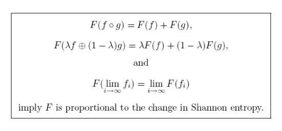
1. Introduction
The Shannon entropy [1] of a probability measure p on a finite set X is given by:
There are many theorems that seek to characterize Shannon entropy starting from plausible assumptions; see for example the book by Aczél and Daróczy [2]. Here we give a new and very simple characterization theorem. The main novelty is that we do not focus directly on the entropy of a single probability measure, but rather, on the change in entropy associated with a measure-preserving function. The entropy of a single probability measure can be recovered as the change in entropy of the unique measure-preserving function onto the one-point space.
A measure-preserving function can map several points to the same point, but not vice versa, so this change in entropy is always a decrease. Since the second law of thermodynamics speaks of entropy increase, this may seem counterintuitive. It may seem less so if we think of the function as some kind of data processing that does not introduce any additional randomness. Then the entropy can only decrease, and we can talk about the “information loss” associated with the function.
Some examples may help to clarify this point. Consider the only possible map . Suppose p is the probability measure on such that each point has measure , while q is the unique probability measure on the set . Then , while . The information loss associated with the map f is defined to be , which in this case equals . In other words, the measure-preserving map f loses one bit of information.
On the other hand, f is also measure-preserving if we replace p by the probability measure for which a has measure 1 and b has measure 0. Since , the function f now has information loss . It may seem odd to say that f loses no information: after all, it maps a and b to the the same point. However, because the point b has probability zero with respect to , knowing that lets us conclude that with probability one.
The shift in emphasis from probability measures to measure-preserving functions suggests that it will be useful to adopt the perspective of category theory [3], where one has objects and morphisms between them. However, the reader need only know the definition of “category” to understand this paper.
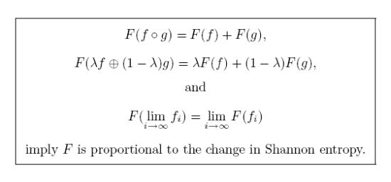
Our main result is that Shannon entropy has a very simple characterization in terms of information loss. To state it, we consider a category where a morphism is a measure-preserving function between finite sets equipped with probability measures. We assume F is a function that assigns to any such morphism a number , which we call its information loss. We also assume that F obeys three axioms. If we call a morphism a “process” (to be thought of as deterministic), we can state these roughly in words as follows. For the precise statement, including all the definitions, see Section 2.
The charm of this result is that the first two hypotheses look like linear conditions, and none of the hypotheses hint at any special role for the function , but it emerges in the conclusion. The key here is a result of Faddeev [4] described in Section 4.
- (i)
- Functoriality. Given a process consisting of two stages, the amount of information lost in the whole process is the sum of the amounts lost at each stage:
- (ii)
- Convex linearity. If we flip a probability-λ coin to decide whether to do one process or another, the information lost is λ times the information lost by the first process plus times the information lost by the second:
- (iii)
- Continuity. If we change a process slightly, the information lost changes only slightly: is a continuous function of f.
For many scientific purposes, probability measures are not enough. Our result extends to general measures on finite sets, as follows. Any measure on a finite set can be expressed as for some scalar λ and probability measure p, and we define . In this more general setting, we are no longer confined to taking convex linear combinations of measures. Accordingly, the convex linearity condition in our main theorem is replaced by two conditions: additivity () and homogeneity (). As before, the conclusion is that, up to a multiplicative constant, F assigns to each morphism the information loss .
It is natural to wonder what happens when we replace the homogeneity axiom by a more general homogeneity condition:
for some number . In this case we find that is proportional to , where is the so-called Tsallis entropy of order α.
2. The Main Result
We work with finite sets equipped with probability measures. All measures on a finite set X will be assumed nonnegative and defined on the σ-algebra of all subsets of X. Any such measure is determined by its values on singletons, so we will think of a probability measure p on X as an X-tuple of numbers () satisfying .
Definition 1. Let be the category where an object is given by a finite set X equipped with a probability measure p, and where a morphism is a measure-preserving function from to , that is, a function such that
for all .
We will usually write an object as p for short, and write a morphism as simply .
There is a way to take convex linear combinations of objects and morphisms in . Let and be finite sets equipped with probability measures, and let . Then there is a probability measure
on the disjoint union of the sets X and Y, whose value at a point k is given by
Given morphisms and , there is a unique morphism
that restricts to f on the measure space p and to g on the measure space q.
The same notation can be extended, in the obvious way, to convex combinations of more than two objects or morphisms. For example, given objects of and nonnegative scalars summing to 1, there is a new object .
Recall that the Shannon entropy of a probability measure p on a finite set X is
with the convention that .
Theorem 2. Suppose F is any map sending morphisms in to numbers in and obeying these three axioms:
where is the Shannon entropy of p. Conversely, for any constant , this formula determines a map F obeying Conditions (i)–(iii).
- (i)
- Functoriality:whenever are composable morphisms.
- (ii)
- Convex linearity:for all morphisms and scalars .
- (iii)
- Continuity: F is continuous.
We need to explain Condition (iii). A sequence of morphisms
in converges to a morphism if:
- for all sufficiently large n, we have , , and for all ;
- and pointwise.
The proof of Theorem 2 is given in Section 5. First we show how to deduce a characterization of Shannon entropy for general measures on finite sets.
The following definition is in analogy to Definition 1:
Definition 3. Let be the category whose objects are finite sets equipped with measures and whose morphisms are measure-preserving functions.
There is more room for maneuver in than in : we can take arbitrary nonnegative linear combinations of objects and morphisms, not just convex combinations. Any nonnegative linear combination can be built up from direct sums and multiplication by nonnegative scalars, which are defined as follows.
- For direct sums, first note that the disjoint union of two finite sets equipped with measures is another object of the same type. We write the disjoint union of as . Then, given morphisms , there is a unique morphism that restricts to f on the measure space p and to g on the measure space q.
- For scalar multiplication, first note that we can multiply a measure by a nonnegative real number and get a new measure. So, given an object and a number we obtain an object with the same underlying set and with . Then, given a morphism , there is a unique morphism that has the same underlying function as f.
We wish to give some conditions guaranteeing that a map sending morphisms in to nonnegative real numbers comes from a multiple of Shannon entropy. To do this we need to define the Shannon entropy of a finite set X equipped with a measure p, not necessarily a probability measure. Define the total mass of to be
If this is nonzero, then p is of the form for a unique probability measure space . In that case we define the Shannon entropy of p to be . If the total mass of p is zero, we define its Shannon entropy to be zero.
We can define continuity for a map sending morphisms in to numbers in just as we did for , and show:
Corollary 4. Suppose F is any map sending morphisms in to numbers in and obeying these four axioms:
where is the Shannon entropy of p. Conversely, for any constant , this formula determines a map F obeying Conditions (i)–(iv).
- (i)
- Functoriality:whenever are composable morphisms.
- (ii)
- Additivity:for all morphisms .
- (iii)
- Homogeneity:for all morphisms f and all .
- (iv)
- Continuity: F is continuous.
Proof. Take a map F obeying these axioms. Then F restricts to a map on morphisms of obeying the axioms of Theorem 2. Hence there exists a constant such that whenever is a morphism between probability measures. Now take an arbitrary morphism in . Since f is measure-preserving, , say. If then , and for some morphism in ; then by homogeneity,
If then , so by homogeneity. So in either case. The converse statement follows from the converse in Theorem 2. ☐
3. Why Shannon Entropy Works
To prove the easy half of Theorem 2, we must check that really does determine a functor obeying all the conditions of that theorem. Since all these conditions are linear in F, it suffices to consider the case where . It is clear that F is continuous, and Equation (1) is also immediate whenever , , are morphisms in :
The work is to prove Equation (2).
We begin by establishing a useful formula for , where as usual f is a morphism in . Since f is measure-preserving, we have
So
where in the last step we note that summing over all i that map to j and then summing over all j is the same as summing over all i. So,
and thus
where the quantity in the sum is defined to be zero when . If we think of p and q as the distributions of random variables and with , then is exactly the conditional entropy of x given y. So, what we are calling “information loss” is a special case of conditional entropy.
This formulation makes it easy to check Equation (2),
simply by applying (5) on both sides.
In the proof of Corollary 4 (on ), the fact that satisfies the four axioms was deduced from the analogous fact for . It can also be checked directly. For this it is helpful to note that
It can then be shown that Equation (5) holds for every morphism f in . The additivity and homogeneity axioms follow easily.
4. Faddeev’s Theorem
To prove the hard part of Theorem 2, we use a characterization of entropy given by Faddeev [4] and nicely summarized at the beginning of a paper by Rényi [5]. In order to state this result, it is convenient to write a probability measure on the set as an n-tuple . With only mild cosmetic changes, Faddeev’s original result states:
Theorem 5. (Faddeev) Suppose I is a map sending any probability measure on any finite set to a nonnegative real number. Suppose that:
- (i)
- I is invariant under bijections.
- (ii)
- I is continuous.
- (iii)
- For any probability measure p on a set of the form , and any number ,
In Condition (i) we are using the fact that given a bijection between finite sets and a probability measure on X, there is a unique probability measure on such that p is measure-preserving; we demand that I takes the same value on both these probability measures. In Condition (ii), we use the standard topology on the simplex
to put a topology on the set of probability distributions on any n-element set.
The most interesting condition in Faddeev’s theorem is (iii). It is known in the literature as the “grouping rule” ([6], Section 2.179)or “recursivity” ([2], Section 1.2.8). It is a special case of “strong additivity” ([2], Section 1.2.6), which already appears in the work of Shannon [1] and Faddeev [4]. Namely, suppose that p is a probability measure on the set . Suppose also that for each , we have a probability measure on a finite set . Then is again a probability measure space, and the Shannon entropy of this space is given by the strong additivity formula:
This can easily be verified using the definition of Shannon entropy and elementary properties of the logarithm. Moreover, Condition (iii) in Faddeev’s theorem is equivalent to strong additivity together with the condition that , allowing us to reformulate Faddeev’s theorem as follows:
Theorem 6. Suppose I is a map sending any probability measure on any finite set to a nonnegative real number. Suppose that:
- (i)
- I is invariant under bijections.
- (ii)
- I is continuous.
- (iii)
- , where is our name for the unique probability measure on the set .
- (iv)
- For any probability measure p on the set and probability measures on finite sets, we have
Proof. Since we already know that the multiples of Shannon entropy have all these properties, we just need to check that Conditions (iii) and (iv) imply Faddeev’s equation (7). Take , and for : then Condition (iv) gives
which by Condition (iii) gives Faddeev’s equation.
It may seem miraculous how the formula
emerges from the assumptions in either Faddeev’s original Theorem 5 or the equivalent Theorem 6. We can demystify this by describing a key step in Faddeev’s argument, as simplified by Rényi [5]. Suppose I is a function satisfying the assumptions of Faddeev’s result. Let
equal I applied to the uniform probability measure on an n-element set. Since we can write a set with elements as a disjoint union of m different n-element sets, Condition (iv) of Theorem 6 implies that
The conditions of Faddeev’s theorem also imply
and the only solutions of both these equations are
This is how the logarithm function enters. Using Condition (iii) of Theorem 5, or equivalently Conditions (iii) and (iv) of Theorem 6, the value of I can be deduced for probability measures p such that each is rational. The result for arbitrary probability measures follows by continuity.
5. Proof of the Main Result
Now we complete the proof of Theorem 2. Assume that F obeys Conditions (i)–(iii) in the statement of this theorem.
Recall that denotes the set equipped with its unique probability measure. For each object , there is a unique morphism
We can think of this as the map that crushes p down to a point and loses all the information that p had. So, we define the “entropy” of the measure p by
Given any morphism in , we have
So, by our assumption that F is functorial,
or in other words:
To conclude the proof, it suffices to show that I is a multiple of Shannon entropy.
We do this by using Theorem 6. Functoriality implies that when a morphism f is invertible, . Together with (8), this gives Condition (i) of Theorem 6. Since is invertible, it also gives Condition (iii). Condition (ii) is immediate. The real work is checking Condition (iv).
Given a probability measure p on together with probability measures on finite sets , respectively, we obtain a probability measure on the disjoint union of . We can also decompose p as a direct sum:
Define a morphism
Then by convex linearity and the definition of I,
But also
by (8) and (9). Comparing these two expressions for gives Condition (iv) of Theorem 6, which completes the proof of Theorem 2.
6. A Characterization of Tsallis Entropy
Since Shannon defined his entropy in 1948, it has been generalized in many ways. Our Theorem 2 can easily be extended to characterize one family of generalizations, the so-called “Tsallis entropies”. For any positive real number α, the Tsallis entropy of order α of a probability measure p on a finite set X is defined as:
The peculiarly different definition when is explained by the fact that the limit exists and equals the Shannon entropy .
Although these entropies are most often named after Tsallis [7], they and related quantities had been studied by others long before the 1988 paper in which Tsallis first wrote about them. For example, Havrda and Charvát [8] had already introduced a similar formula, adapted to base 2 logarithms, in a 1967 paper in information theory, and in 1982, Patil and Taillie [9] had used itself as a measure of biological diversity.
The characterization of Tsallis entropy is exactly the same as that of Shannon entropy except in one respect: in the convex linearity condition, the degree of homogeneity changes from 1 to α.
Theorem 7. Let . Suppose F is any map sending morphisms in to numbers in and obeying these three axioms:
where is the order α Tsallis entropy of p. Conversely, for any constant , this formula determines a map F obeying Conditions (i)–(iii).
- (i)
- Functoriality:whenever are composable morphisms.
- (ii)
- Compatibility with convex combinations:for all morphisms and all .
- (iii)
- Continuity: F is continuous.
Proof. We use Theorem V.2 of Furuichi [10]. The statement of Furuichi’s theorem is the same as that of Theorem 5 (Faddeev’s theorem), except that Condition (iii) is replaced by
and Shannon entropy is replaced by Tsallis entropy of order α. The proof of the present theorem is thus the same as that of Theorem 2, except that Faddeev’s theorem is replaced by Furuichi’s. ☐
As in the case of Shannon entropy, this result can be extended to arbitrary measures on finite sets. For this we need to define the Tsallis entropies of an arbitrary measure on a finite set. We do so by requiring that
for all and all . When this is the same as the Shannon entropy, and when , we have
(which is analogous to (6)). The following result is the same as Corollary 4 except that, again, the degree of homogeneity changes from 1 to α.
Corollary 8. Let . Suppose F is any map sending morphisms in to numbers in , and obeying these four properties:
where is the Tsallis entropy of order α. Conversely, for any constant , this formula determines a map F obeying Conditions (i)–(iv).
- (i)
- Functoriality:whenever are composable morphisms.
- (ii)
- Additivity:for all morphisms .
- (iii)
- Homogeneity of degree:for all morphisms f and all .
- (iv)
- Continuity: F is continuous.
Proof. This follows from Theorem 7 in just the same way that Corollary 4 follows from Theorem 2. ☐
Acknowledgements
We thank the denizens of the n-Category Café, especially David Corfield, Steve Lack, Mark Meckes and Josh Shadlen, for encouragement and helpful suggestions. Tobias Fritz is supported by the EU STREP QCS. Tom Leinster is supported by an EPSRC Advanced Research Fellowship.
References
- Shannon, C.E. A mathematical theory of communication. Bell Syst. Tech. J. 1948, 27, 379–423. [Google Scholar] [CrossRef]
- Aczél, J.; Daróczy, Z. On Measures of information and their characterizations. In Mathematics in Science and Engineering; Academic Press: New York, NY, USA, 1975; Volume 15. [Google Scholar]
- Mac Lane, S. Categories for the working mathematician. In Graduate Texts in Mathematics 5; Springer: Berlin, Germany, 1971. [Google Scholar]
- Faddeev, D.K. On the concept of entropy of a finite probabilistic scheme. Uspehi Mat. Nauk (N.S.) 1956, 1, 227–231. (In Russian) [Google Scholar]
- Rényi, A. Measures of information and entropy. In Proceedings of the 4th Berkeley Symposium on Mathematical Statistics and Probability, Statistical Laboratory of the University of California, Berkeley, CA, USA, June 20–July 30, 1960; University of California Press: Berkeley, CA, USA, 1961; pp. 547–561. [Google Scholar]
- Cover, T.M.; Thomas, J.A. Elements of Information Theory; Wiley Series in Telecommunications and Signal Processing; Wiley-Interscience: New York, NY, USA, 2006. [Google Scholar]
- Tsallis, C. Possible generalization of Boltzmann-Gibbs statistics. J. Stat. Phys. 1988, 52, 479–487. [Google Scholar] [CrossRef]
- Havrda, J.; Charvát, F. Quantification method of classification processes: concept of structural α-entropy. Kybernetika 1967, 3, 30–35. [Google Scholar]
- Patil, G.P.; Taillie, C. Diversity as a concept and its measurement. J. Am. Stat. Assoc. 1982, 77, 548–561. [Google Scholar] [CrossRef]
- Furuichi, S. On uniqueness theorems for Tsallis entropy and Tsallis relative entropy. IEEE Trans. Infor. Theor. 2005, 51, 3638–3645. [Google Scholar] [CrossRef]
© 2011 by the authors; licensee MDPI, Basel, Switzerland. This article is an open access article distributed under the terms and conditions of the Creative Commons Attribution license (http://creativecommons.org/licenses/by/3.0/).
Share and Cite
MDPI and ACS Style
Baez, J.C.; Fritz, T.; Leinster, T. A Characterization of Entropy in Terms of Information Loss. Entropy 2011, 13, 1945-1957. https://doi.org/10.3390/e13111945
AMA Style
Baez JC, Fritz T, Leinster T. A Characterization of Entropy in Terms of Information Loss. Entropy. 2011; 13(11):1945-1957. https://doi.org/10.3390/e13111945
Chicago/Turabian StyleBaez, John C., Tobias Fritz, and Tom Leinster. 2011. "A Characterization of Entropy in Terms of Information Loss" Entropy 13, no. 11: 1945-1957. https://doi.org/10.3390/e13111945