Fluctuation, Dissipation and the Arrow of Time

Abstract

The recent development of the theory of fluctuation relations has led to new insights into the ever-lasting question of how irreversible behavior emerges from time-reversal symmetric microscopic dynamics. We provide an introduction to fluctuation relations, examine their relation to dissipation and discuss their impact on the arrow of time question.

1. Introduction

Irreversibility enters the laws of thermodynamics in two distinct ways:

Equilibrium Principle 

An isolated, macroscopic system which is placed in an arbitrary initial state within a finite fixed volume will attain a unique state of equilibrium.

Second Law (Clausius) 

For a non-quasi-static process occurring in a thermally isolated system, the entropy change between two equilibrium states is non-negative.

The first of these two principles is the Equilibrium Principle [1], whereas the second is the Second Law of Thermodynamics in the formulation given by Clausius [2,3]. Very often the Equilibrium Principle is loosely referred to as the Second Law of Thermodynamics, thus creating a great confusion in the literature. So much that proposing to raise the Equilibrium Principle to the rank of one of the fundamental laws of thermodynamic became necessary [1]. Indeed it was argued that this Law of Thermodynamics, defining the very concept of state of equilibrium, is the most fundamental of all the Laws of Thermodynamics (which in fact are formulated in terms of equilibrium states) and for this reason the nomenclature Minus-First Law of Thermodynamics was proposed for it.

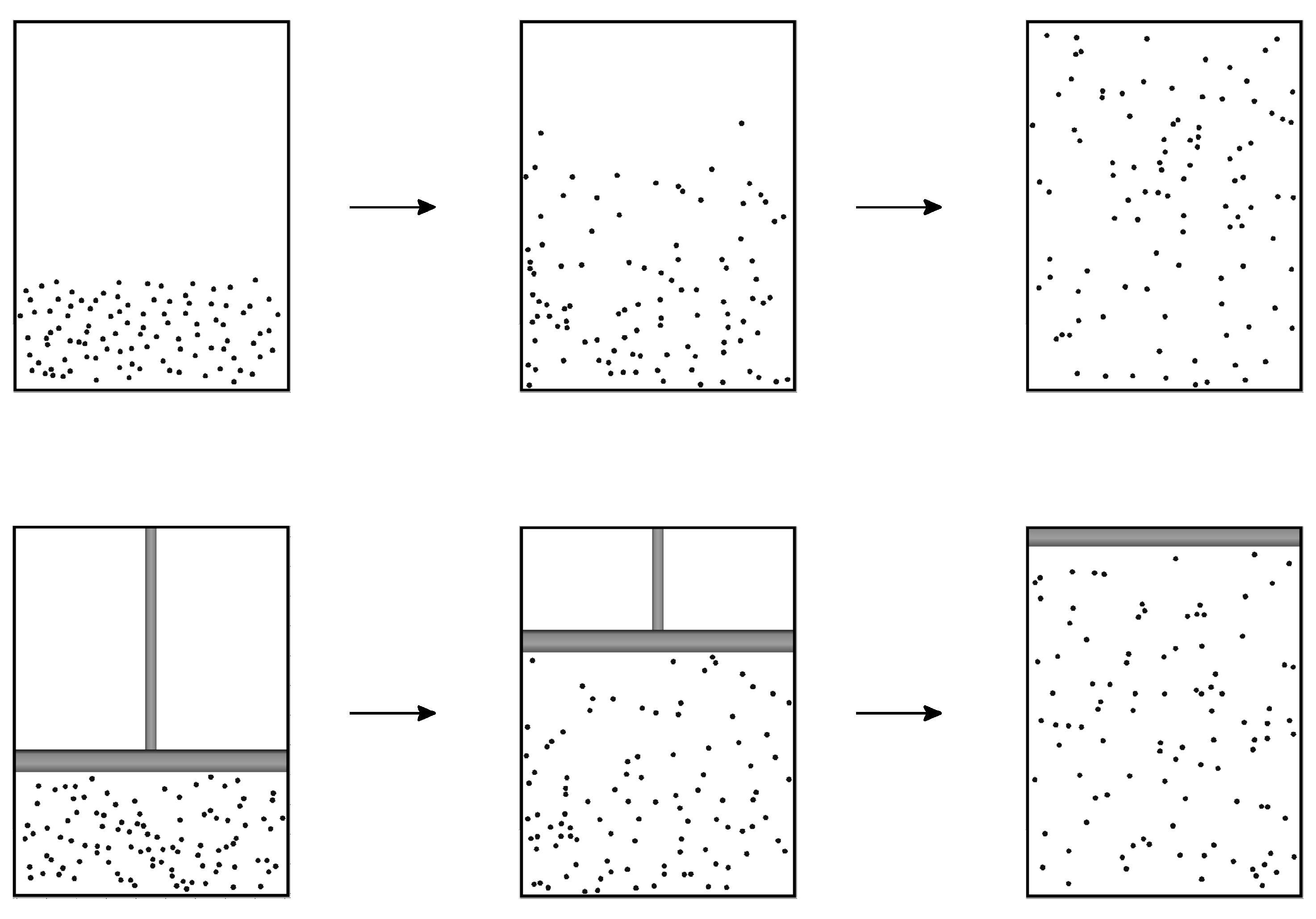
The Minus-First Law of Thermodynamics and the Second Law of Thermodynamics consider two very different situations, see Figure 1. The Minus-First Law deals with a completely isolated system that begins in non-equilibrium and ends in equilibrium, following its spontaneous and autonomous evolution. In the Second Law one considers a thermally (but not mechanically) isolated system that begins in equilibrium. A time-dependent mechanical action perturbs the initial equilibrium, the action is then turned off and a final equilibrium will be reached, corresponding to higher entropy [4]. At variance with the Minus-First Law, here the system does not evolve autonomously, but rather in response to a driving: we speak in this case of nonautonomous evolution.

The use of the qualifiers “autonomous” and “nonautonomous” reflects here the fact that the set of differential equations describing the microscopic evolution of the system are autonomous (i.e., they do not contain time explicitly) in cases of the type depicted in Figure 1, top, and are nonautonomous (i.e., they contain time explictely) in cases of the type depicted in Figure 1, bottom. Accordingly the Hamilton function is time independent in the former cases and time dependent in the latter ones (see Section 2 below).

Figure 1. Autonomous vs. nonautonomous dynamics. Top: Autonomous evolution of a gas from a non-equilibrium state to an equilibrium state (Minus-First Law). Bottom: Nonautonomous evolution of a thermally isolated gas between two equilibrium states. The piston moves according to a pre-determined protocol specifying its position ${\lambda }_t$ in time. The entropy change is non-negative (Second Law).

Figure 1. Autonomous vs. nonautonomous dynamics. Top: Autonomous evolution of a gas from a non-equilibrium state to an equilibrium state (Minus-First Law). Bottom: Nonautonomous evolution of a thermally isolated gas between two equilibrium states. The piston moves according to a pre-determined protocol specifying its position ${\lambda }_t$ in time. The entropy change is non-negative (Second Law).

In order to illustrate the necessity of clearly distinguishing between the two prototypical evolutions depicted in Figure 1, let us analyze one statement which is often referred to as the second law: after the removal of a constraint, a thermally isolated system that is initially in equilibrium reaches a new equilibrium at higher entropy [5]. While, after the removal of the constraint the system evolves autonomously (hence, in accordance to the equilibrium principle it will eventually reach a unique equilibrium state), it is often overlooked the fact that the overall process is nevertheless described by a set of nonautonomous differential equations (because the removal of the constraint is an instance of an external time-dependent mechanical intervention) with the constrained equilibrium as initial state. Then, in accordance with Clausius principle the final state is of higher or same entropy. Thus, this formulation of the second law can be seen as a special case of Clausius formulation that considers only those external interventions which are called constraint removals.

Both the Minus-First Law and the Second Law have to do with irreversibility and the arrow of time. While since the seminal works of Boltzmann, the main efforts of those working in the foundations of statistical mechanics were directed to reconcile the Minus-First Law with the time-reversal symmetric microscopic dynamics, recent developments in the theory of fluctuation relations have brought new and deep insights into the microscopic foundations of the Second Law. As we shall see below, fluctuation theorems highlight in a most clear way the fascinating fact that the Second Law is deeply rooted in the time-reversal symmetric nature of the laws of microscopic dynamics [6,7].

This connection is best seen if one considers the Second Law in the formulation given by Kelvin, which is equivalent to Clausius formulation [8]:

Second Law (Kelvin) 

No work can be extracted from a closed equilibrium system during a cyclic variation of a parameter by an external source.

The field of fluctuation theorems has recently gained much attention. Many fluctuation theorems have been reported in the literature, referring to different scenarios. Fluctuation theorems exist for classical dynamics, stochastic dynamics, and for quantum dynamics; for transiently driven systems, as well as for non-equilibrium steady states; for systems prepared in canonical, micro-canonical, grand-canonical ensembles, and even for systems initially in contact with “finite heat baths” [9]; they can refer to different quantities like work (different kinds), entropy production, exchanged heat, exchanged charge, and even information, depending on different set-ups. All these developments including discussions of the experimental applications of fluctuation theorems have been summarized in a number of reviews [6,7,10,11].

In Section 2 we will give a brief introduction to the classical work Fluctuation Theorem of Bochkov and Kuzovlev [12], which is the first fluctuation theorem reported in the literature. The discussion of this theorem suffices for our purpose of highlighting the impact of fluctuation theory on dissipation (Section 3) and on the arrow of time issue (Section 4). Remarks of the origin of time’s arrow in this context are collected in Section 5.

2. The Fluctuation Theorem

2.1. Autonomous Dynamics

Consider a completely isolated mechanical system composed of f degrees of freedom. Its dynamics are dictated by some time independent Hamiltonian $H(\mathbf{q},\mathbf{p})$, which we assume to be time reversal symmetric; i.e.,

$$H(\mathbf{q},\mathbf{p})=H(\mathbf{q},-\mathbf{p})$$

(1)

Here $(\mathbf{q},\mathbf{p})=(q_1\cdots q_f,p_1\cdots p_f)$ denotes the conjugate pairs of coordinates and momenta describing the microscopic state of the system.

The assumption of time-reversal symmetry implies that if $[\mathbf{q}(t),\mathbf{p}(t)]$ is a solution of Hamilton equations of motion, then, for any τ, $[\mathbf{q}(\tau -t),-\mathbf{p}(\tau -t)]$ is also a solution of Hamilton equations of motion. This is the well known principle of microreversibility for autonomous systems [13].

We assume that the system is at equilibrium described by the Gibbs ensemble:

$$\varrho (\mathbf{q},\mathbf{p})=e^{-\beta H(\mathbf{q},\mathbf{p})}/Z\left(\beta \right)$$

(2)

where $Z\left(\beta \right)=\int d\mathbf{p}d\mathbf{q}{e}^{-\beta H(\mathbf{q},\mathbf{p})}$ is the canonical partition function, and ${\beta }^{-1}=k_{B}T$, with $k_B$ being the Boltzmann constant and T denotes the temperature.

We next imagine to be able to observe the time evolution of all coordinates and momenta within some time span $t\in [0,\tau ]$. Fluctuation theorems are concerned with the probability [14] $P[\Gamma ]$ that the trajectory Γ is observed. We will reserve the symbol Γ to denote the whole trajectory (that is, mathematically speaking, to denote a map from the interval $[0,\tau ]$ to the $2f$ dimensional phase space), whereas the symbol ${\Gamma }_t$ will be used to denote the specific point in phase space visited by the trajectory Γ at time t. The central question is how the probability $P[\Gamma ]$ compares with the probability $P[\tilde{\Gamma }]$ to observe $\tilde{\Gamma }$, the time-reversal companion of Γ: ${\tilde{\Gamma }}_t=\epsilon {\Gamma }_{\tau -t}$ where $\epsilon (\mathbf{q},\mathbf{p})=(\mathbf{q},-\mathbf{p})$ denotes the time reversal operator. The answer is given by the microreversibility principle which implies:

$$P[\Gamma ]=P[\tilde{\Gamma }]$$

(3)

To see this, consider the Hamiltonian dynamics but for the case that the trajectory Γ is not a solution of Hamilton equations, then $\tilde{\Gamma }$ is also not a solution, and both the probabilities $P[\Gamma ]$ and $P[\tilde{\Gamma }]$ are trivially zero. Now consider the case when Γ is solution of Hamilton equations, then also $\tilde{\Gamma }$ is a solution. Since the dynamics are Hamiltonian, there is one and only one solution passing through the point ${\Gamma }_0$ at time $t=0$, then the probability $P[\Gamma ]$ is given by the probability to observe the system at ${\Gamma }_0$ at $t=0$. By our equilibrium assumption this is given by $\varrho \left({\Gamma }_0\right)$ [15]. Likewise the $P[\tilde{\Gamma }]$ is given by $\varrho \left({\tilde{\Gamma }}_0\right)$. Due to time-reversal symmetry and energy conservation we have $H\left({\tilde{\Gamma }}_0\right)=H\left(\epsilon {\Gamma }_{\tau }\right)=H\left({\Gamma }_{\tau }\right)=H\left({\Gamma }_0\right)$ implying $\varrho \left({\tilde{\Gamma }}_0\right)=\varrho \left({\Gamma }_0\right)$, hence Equation (3).

To summarize, the microreversibility principle for autonomous systems in conjunction with the hypothesis of Gibbsian equilibrium implies that the probability to observe a trajectory and its time-reversal companion are equal. There is no way to distinguish between past and future in an autonomous system at equilibrium. Obviously, this is no longer so when the system is prepared out of equilibrium, as in Figure 1, top.

2.2. Nonautonomous Dynamics

Imagine now the nonautonomous case of a thermally insulated system driven through the variation of a parameter ${\lambda }_t$. Thermal insulation guarantees that the dynamics are still Hamiltonian. At variance with the autonomous case though, now the Hamiltonian is time dependent. Without loss of generality we assume that the varying parameter, denoted by ${\lambda }_t$ couples linearly to some system observable $Q(\mathbf{q},\mathbf{p})$, so that the Hamiltonian reads:

$$H(\mathbf{q},\mathbf{p};{\lambda }_t)=H_0(\mathbf{q},\mathbf{p})-{\lambda }_{t}Q(\mathbf{q},\mathbf{p})$$

(4)

This is the traditional form employed in the study of the fluctuation-dissipation theorem [16,17]. In the following we shall reserve the symbol λ (without subscript) to denote the whole parameter variation protocol, and use the symbol ${\lambda }_t$, to denote the specific value taken by the parameter at time t. The succession of parameter values is assumed to be pre-specified (the system evolution does not affect the parameter evolution).

We assume that ${\lambda }_t=0$ for $t=0$ and that the system is prepared at $t=0$ in the equilibrium Gibbs state

$${\varrho }_0(\mathbf{q},\mathbf{p})=e^{-\beta H_0(\mathbf{q},\mathbf{p})}/Z_0\left(\beta \right)$$

(5)

where $Z_0\left(\beta \right)=\int \mathrm{d}\mathbf{q}\mathrm{d}\mathbf{q}{e}^{-\beta H_0(\mathbf{q},\mathbf{p})}$. We further assume that at any fixed value of the parameter the Hamiltonian is time reversal symmetric:

$$H(\mathbf{q},\mathbf{p};{\lambda }_t)=H(\mathbf{q},-\mathbf{p};{\lambda }_t)$$

(6)

Note here the fact that energy is not conserved in the nonautonomous case because the Hamiltonian is time-dependent in this case. Microreveresibility, as we have described it above, also does not hold: Given a protocol λ, if Γ is a solution of the Hamilton equations of motion, in general $\tilde{\Gamma }$ is not. However $\tilde{\Gamma }$ is a solution of the equations of motion generated by the time-reversed protocol $\tilde{\lambda }$, where ${\tilde{\lambda }}_t={\lambda }_{\tau -t}$. This is the microreversibility principle for nonautonmous systems [6]. It is illustrated in Figure 2. Despite its importance we are not aware of any textbooks in classical (or quantum) mechanics that discusses it. A classical proof appears in [18] (Section 1.2.3). Corresponding quantum proofs were given in [19] and in Appendix B of [6].

As with the autonomous case we can ask how the probability distribution $P[\Gamma ,\lambda ]$ that the trajectory Γ is realized under the protocol λ, compares with the probability distribution $P[\tilde{\Gamma },\tilde{\lambda }]$ that the reversed trajectory $\tilde{\Gamma }$ is realized under the reversed protocol $\tilde{\lambda }$. The answer to this was first given by Bochkov and Kuzovlev [12], who showed that

$$P[\Gamma ,\lambda ]=P[\tilde{\Gamma },\tilde{\lambda }]e^{\beta W_0}$$

(7)

where

$$W_0={\int }_0^{\tau }dt{\lambda }_t{\dot{Q}}_t$$

(8)

Here, $Q_t=Q\left({\Gamma }_t\right)$ denotes the evolution of the quantity Q along the trajectory Γ and $W_0$ is the so called “exclusive work”. As discussed in [6,20,21,22] yet another definition of work is possible, the so called “inclusive work” $W=-\int dt{\dot{\lambda }}_t{Q}_t$, leading to a different and equally important fluctuation theorem involving free energy differences [6,23,24]. Without entering the question about the physical meaning of the two quantities W and $W_0$, it suffices for the present purpose to notice that for a cyclic transformation $W_0=W$ [25]. In the remaining of this section we will restrict our analysis to cyclic transformations (${\lambda }_0={\lambda }_{\tau }$) in order to make contact with Kelvin postulate and to avoid any ambiguity regarding the usage of the word “work”.

Figure 2. Microreversibility for nonautonomous classical (Hamiltonian) systems. The initial condition ${\Gamma }_0$ evolves to ${\Gamma }_{\tau }$ under the protocol λ, following the path Γ. The time-reversed final condition $\epsilon {\Gamma }_{\tau }$ evolves to the time-reversed initial condition $\epsilon {\Gamma }_0$ under the protocol $\tilde{\lambda }$, following the path $\tilde{\Gamma }$.

Figure 2. Microreversibility for nonautonomous classical (Hamiltonian) systems. The initial condition ${\Gamma }_0$ evolves to ${\Gamma }_{\tau }$ under the protocol λ, following the path Γ. The time-reversed final condition $\epsilon {\Gamma }_{\tau }$ evolves to the time-reversed initial condition $\epsilon {\Gamma }_0$ under the protocol $\tilde{\lambda }$, following the path $\tilde{\Gamma }$.

Just like Equation (3) constitutes a direct expression of the principle of microreversibility for autonomous systems, so is Equation (7) a direct expression of the more general principle of microreversibility for nonautonomous systems. Remarkably it expresses the second law in a most clear and refined way.

In order to see this, it is important to realize that the work $W_0$ is odd under time-reversal. This is so because $W_0$ is linear in a quantity ${\dot{Q}}_t$, which is the time derivative of an even observable Q. The theorem says that the probability to observe a trajectory corresponding to some work $W_0>0$ under the driving λ is exponentially larger than the probability to observe the reversed trajectory (corresponding to $-W_0$) under the driving $\tilde{\lambda }$. This provides a statistical formulation of the second law

Second Law (Fluctuation Theorem) 

Injecting some amount of energy $W_0$ into a thermally insulated system at equilibrium at temperature T by the cyclic variation of a parameter, is exponentially (i.e., by a factor $e^{W_0/\left(k_{B}T\right)}$) more probable than withdrawing the same amount of energy from it by the reversed parameter variation.

Multiplying Equation (7) by $e^{-\beta W_0}$ and integrating over all Γ-trajectories leads to the relation [12]:

$${\langle e^{-\beta W_0}\rangle }_{\lambda }=1$$

(9)

The subscript λ in Equation (9) is there to recall that the average is taken over the trajectories generated by the protocol λ. In particular, the notation ${\langle ·\rangle }_{\lambda }$ denotes a nonequilibrium average [26]. Combining Equation (9) with Jensen’s inequality, $\langle exp\left(x\right)\rangle \ge exp(\langle x\rangle )$ leads to

$${\langle W_0\rangle }_{\lambda }\ge 0$$

(10)

which now expresses Kelvin’s postulate as a nonequilibrium inequality [12]. The quantum version of the fluctuation theorem by Bochkov and Kuzovlev has been given only recently in [22]. This latter reference in addition reports its microcanonical variant, which applies to the case when the system begins in a state of well defined energy.

3. Dissipation: Kubo’s Formula

Before we continue with the implications of the fluctuation theorem for the arrow of time question, it is instructive to see in which way the fluctuation theorem relates to dissipation.

Given the distribution $P[\Gamma ,\lambda ]$, the distribution $p[Q,\lambda ]$ that a trajectory Q of the observable $Q(\mathbf{q},\mathbf{p})$ occurs in the time span $[0,\tau ]$ can be formally expressed as:

$$p[Q,\lambda ]=\int \mathcal{D}\Gamma P[\Gamma ,\lambda ]\delta (Q-Q[\Gamma ])$$

(11)

where δ denotes Dirac’s delta in the Q-trajectory space, the integration is a functional integration over all Γ-trajectories, and $Q[\Gamma ]$ is defined as $Q{[\Gamma ]}_t\doteq Q[{\Gamma }_t]$.

Multiplying Equation (3) by $e^{-\beta \int {\lambda }_s{\dot{Q}}_{s}ds}\delta (Q-Q[\Gamma ])$ and integrating over all Γ-trajectories, one finds:

$$p[Q,\lambda ]e^{-\beta \int {\lambda }_s{\dot{Q}}_{s}ds}=p[\tilde{Q},\tilde{\lambda }]$$

(12)

where $\tilde{Q}$ is the time reversal companion of Q: ${\tilde{Q}}_t=Q_{\tau -t}$. Now multiplying both sides of Equation (12) by $Q_{\tau }$ and integrating over all Q-trajectories, one obtains:

$${\langle Q_{\tau }{e}^{-\beta \int {\lambda }_s{\dot{Q}}_{s}ds}\rangle }_{\lambda }={\langle {\tilde{Q}}_{\tau }\rangle }_{\tilde{\lambda }}$$

(13)

Note that ${\langle {\tilde{Q}}_{\tau }\rangle }_{\tilde{\lambda }}={\langle Q_0\rangle }_{\tilde{\lambda }}$ and that, due to causality, the value taken by the observable $Q(\mathbf{q},\mathbf{p})$ at time $t=0$ cannot be influenced by the subsequent evolution of the protocol $\tilde{\lambda }$. Therefore, the average presents a manifest equilibrium average; that is to say that it is an average over the initial canonical equilibrium ${\varrho }_0(\mathbf{q},\mathbf{p})$. We denote this equilibrium average by the symbol $\langle ·\rangle$ (with no subscript). Thus, Equation (13) reads

$${\langle Q_{\tau }{e}^{-\beta \int {\lambda }_s{\dot{Q}}_{s}ds}\rangle }_{\lambda }=\langle Q_0\rangle$$

(14)

By expanding the exponential in Equation (14) to first order in λ, one obtains:

$$\begin{array}{cc}\hfill {\langle Q_{\tau }\rangle }_{\lambda }-\langle Q_0\rangle & =\beta {〈Q_{\tau }{\int }_0^{\tau }{\lambda }_s{\dot{Q}}_{s}ds〉}_{\lambda }+O\left({\lambda }^2\right)\hfill \end{array}$$

(15)

Since the bracketed expression on the rhs is already $O\left(\lambda \right)$ we can replace the non-equilibrium average ${\langle ·\rangle }_{\lambda }$ with the equilibrium average $\langle ·\rangle$ on the rhs. Further, since averaging commutes with time integration one arrives, up to order $O\left({\lambda }^2\right)$, at:

$$\begin{array}{cc}\hfill {\langle Q_{\tau }\rangle }_{\lambda }-\langle Q_0\rangle & =\beta {\int }_0^{\tau }\langle Q_{\tau }{\dot{Q}}_s\rangle {\lambda }_{s}ds\hfill \end{array}$$

(16)

$$\begin{array}{cc}& =-\beta {\int }_0^{\tau }\langle {\dot{Q}}_{\tau -s}{Q}_0\rangle {\lambda }_{s}ds\hfill \end{array}$$

(17)

In the second line we made use of the time-homogeneous nature of the equilibrium correlation function. This is the celebrated Kubo formula [16] relating the non-equilibrium linear response of the quantity Q to the equilibrium correlation function $\varphi (s,\tau )=\langle Q_{\tau }{\dot{Q}}_s\rangle$. As Kubo showed it implies the fluctuation-dissipation relation [27], linking, for example, the mobility of a Brownian particle to its diffusion coefficient [28], and the resistance of an electrical circuit to its thermal noise [29,30].

This classical derivation of Kubo’s formula from the fluctuation theorem is a simplified version of the derivation given by Bochkov and Kuzovlev [12]. The corresponding quantum derivation was reported by Andrieux and Gaspard [19].

4. Implications for the Arrow of Time Question

Jarzynski has analyzed in a transparent way how the fluctuation theorem for the inclusive work, W, may be employed to make guesses about the direction of time’s arrow [7]. Here we adapt his reasoning to the case of the exclusive work, $W_0$, which appears in the fluctuation relation of Bochkov and Kuzovlev, Equation (7).

Just imagine we are shown a movie of an experiment in which a system starting at temperature $T={\left(k_B\beta \right)}^{-1}$ is driven by a protocol, and we are asked to guess whether the movie is displayed in the same direction as it was filmed or in the backward direction, knowing that tossing of an unbiased coin decided the direction of the movie. When the outcome is $+(-)$, the movie is shown in the same(opposite) direction as it was filmed. Imagine next that we can infer from the analysis of each single frame t the instantaneous values ${\lambda }_t$ and $Q_t$ taken by the parameter and its conjugate observable, respectively. With these we can evaluate the work $W_0$ for the displayed process using Equation (8). Envision that we find, for the shown movie that $\beta W_0\gg 1$. If the film was shown in the “correct” direction it means that a process corresponding to $\beta W_0\gg 1$ occurred. If the film was shown backward then it means that a process corresponding to $\beta W_0\ll -1$ occurred (recall that $W_0$ is odd under time-reversal). The fluctuation theorem tells us that the former case occurs with an overwhelmingly higher probability relative to the probability of the latter case. Then we can be very much confident that the film was running in the correct direction. Likewise if we observe $\beta W_0\ll -1$, then we can say with very much confidence the the film depicts the process in the opposite direction as it happened. Clearly when intermediate values of $\beta W_0$ are observed we can still make well informed guesses about the direction of the movie, but with less confidence. The worst scenario arises when we observe $W_0=0$, in which case we cannot make any reliable guess. The question then arises of how to quantify the confidence of our guesses. This is a typical problem of Bayesian inference. Before we are shown the movie our degree of belief of the outcome + is given by the prior, $P(+)=1/2$ (likewise, $P(-)=1-P(+)=1/2)$. After we have seen the movie the prior is updated to the posterior, $P(+|W_0)$, which is the degree of belief that the outcome + occurred, given the observed work $W_0$. Using Bayes theorem, the posterior is given by

$$P(+|W_0)=\frac{P\left(W_0\right|+)}{P\left(W_0\right)}P(+)$$

(18)

where $P\left(W_0\right|+)$ is the conditional probability to observe $W_0$ given that + occurred, and $P\left(W_0\right)$ is the probability to observe $W_0$; i.e., $P\left(W_0\right)=P\left(W_0\right|+)P(+)+P\left(W_0\right|-)P(-)$. According to the fluctuation theorem $P\left(W_0\right|+)/P(-W_0|+)=e^{\beta W_0}$ and since $W_0$ is odd under time reversal, $P\left(W_0\right|-)=P(-W_0|+)$. Using these relations together with Equation (18) one obtains:

$$P(+|W_0)=\frac{1}{e^{-\beta W_0}+1}$$

(19)

Figure 3. Degree of belief $P(+|W_0)$ that a movie showing the nonautonomous evolution of a system is shown in the same temporal order as it was filmed, given that the work $W_0$ was observed and that the direction of the movie was decided by the tossing of an unbiased coin.

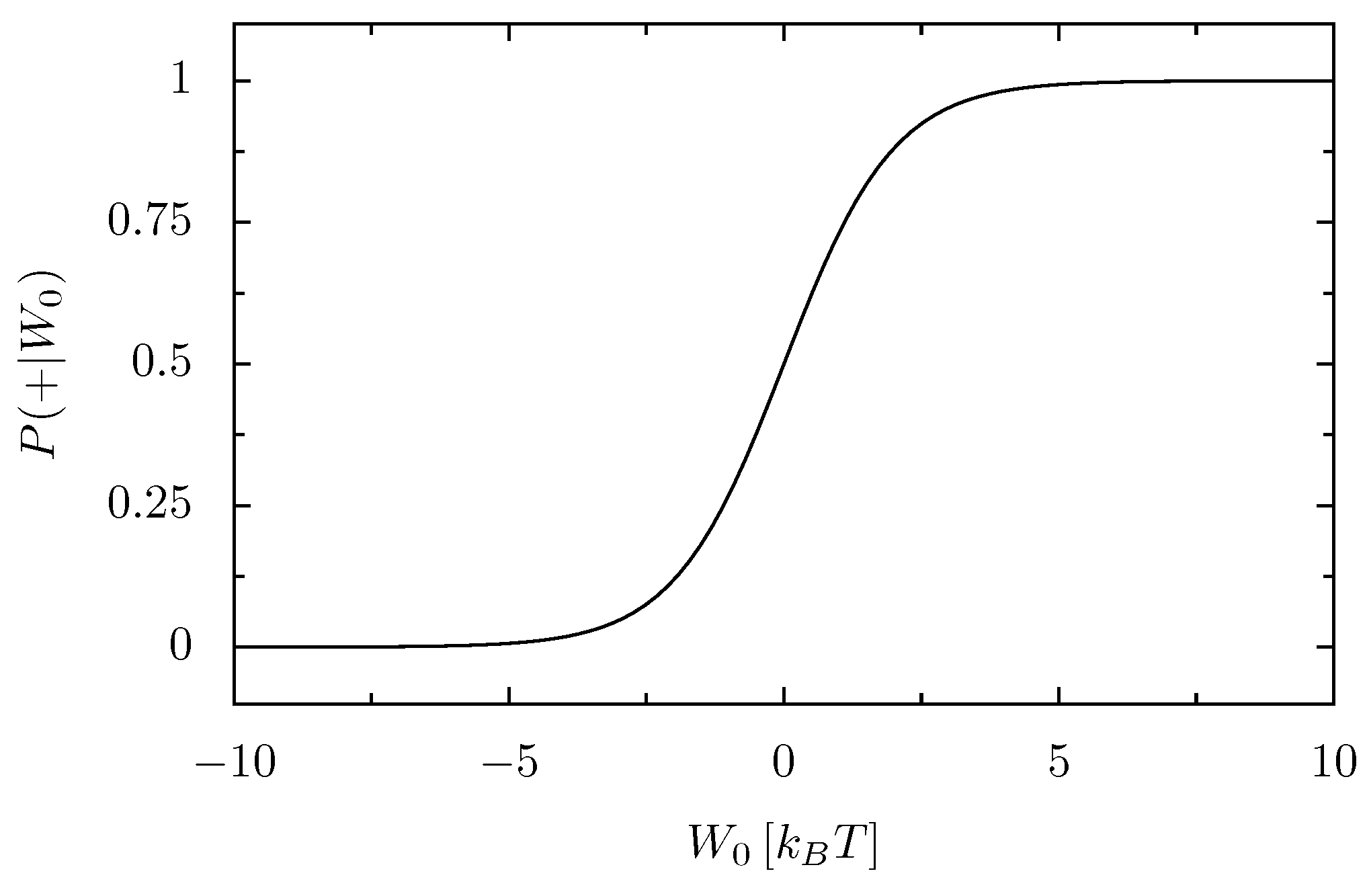
Figure 3. Degree of belief $P(+|W_0)$ that a movie showing the nonautonomous evolution of a system is shown in the same temporal order as it was filmed, given that the work $W_0$ was observed and that the direction of the movie was decided by the tossing of an unbiased coin.

Figure 3 displays $P(+|W_0)$ as a function of $W_0$. As it should be $P(+|W_0)$ is larger than $1/2$ for positive $W_0$ (and vice versa) and is an increasing function of $W_0$. If $W_0$ is large compared to ${\beta }^{-1}$, then $P(+|W_0)\simeq 1$, and we can be almost certain that the movie was shown in the forward direction. Vice versa, if $\beta W_0\ll -1$, then we can say with almost certainty that the movie has been shown backward. The transition to certainty of guess occurs quite rapidly (in fact exponentially) around $|\beta W_0|\simeq 5$. Note that for an autonomous system $W_0=0$, implying $P(+|W_0)=P(-|W_0)=1/2$, meaning that, as we have elaborated above, there is no way to discern the direction of time’s arrow in an autonomous system at equilibrium.

Since the fluctuation theorem (7) holds as a general law regardless of the size of the system, it appears that our ability to discern the direction of time’s arrow does not depend on the system size. It is also worth mentioning the role played by thermal fluctuations in shaping our guesses. Particularly, with a given observed value $W_0$, the lower the temperature, the higher is the confidence (and vice versa).

5. Remarks

It emerges from our discussion regarding the arrow of time (Section 4) that the statistical character of the Second Law becomes visible when the energies injected in a system, $W_0$, are of the same order of magnitude as the thermal fluctuations, $k_{B}T$, regardless of the system size. This means, that, in contrast to what is sometimes believed, work fluctuations happen and are experimentally observable in microscopic and macroscopic systems alike. As a matter of fact, experimental verifications of the fluctuation theorem have been performed involving both microscopic systems, e.g., a single macromolecule [31,32], and macroscopic systems, e.g., a torsional pendulum [33].

As we have mentioned in the introduction, traditionally the question of the emergence of the arrow of time from microscopic dynamics have been addressed within the framework of the Minus-First Law. In all existing approaches the arrow of time emerges from the introduction of some extra ingredient which in turn then dictates the time direction. Typically, one resorts to a coarse-graining procedure of the microscopic phase space to describe some state variables. For example, this is so in the theory of Gibbs and related approaches, see, e.g., in [34]. The time arrow is then generated via the observation that such coarse grained quantities no longer obey time-reversal symmetric Hamiltonian dynamics. More frequently, one resorts to additional assumptions which are of a probabilistic nature: Typical scenarios that come to mind are (i) the use of Boltzmann Stoßahlansatz in the celebrated Boltzmann kinetic theory, (ii) the assumption of initial molecular chaos in more general kinetic theories that are in the spirit of Bogoliubov, or, likewise, with Fokker-Planck and master equation dynamics that no longer exhibit an explicit time-reversal invariant structure [34,35]. All such additional elements then induce the result of a direction in time with future not being equivalent with past any longer.

Having stressed the too often overlooked fact that the Second Law does not refer to the traditionally considered scenario of autonomously evolving systems, but rather to the case of nonautonomous dynamics, here we have focussed on the emergence of time’s arrow in a driven system starting at equilibrium. Having based our derivation on the principle of nonautonomous microreversibility, Figure 2, the question arises naturally regarding the origin of the time asymmetry in this case. It originates from the combination of the following two elements: (i) The introduction of an explicit time dependence of the Hamiltonian, Equation (4), (ii) The particular shape of the initial equilibrium state, Equation (5). The first breaks time homogeneity, thus determining the emergence of an arrow of time, while the second determines its direction. It is in particular the fact that the initial equilibrium is described by a probability density function which is a decreasing function of energy that determines the ≥ sign in Equation (10). An increasing probability density function would result in the opposite sign [8,36,37]. With regard to breaking time homogeneity, it is worth commenting that the assumption of nonautonomous evolution has to be regarded itself as a convenient and often extremely good approximation in which the evolution λ of the external parameter influences the system dynamics without being influenced minimally by the system [38]. This indeed presupposes the intervention of a sort of Maxwell Demon (i.e., the experimentalist), who predisposes things in such a way that the wanted protocol actually occurs. This in turn evidences the phenomenological nature of the Second Law. It is not a law that dictates how things go by themselves, but rather how they go in response to particular experimental investigations.

References and Notes

- Brown, H.R.; Uffink, J. The origins of time-asymmetry in thermodynamics: The minus first law. Stud. Hist. Phil. Mod. Phys. 2001, 32, 525–538. [Google Scholar] [CrossRef]
- Campisi, M. On the mechanical foundations of thermodynamics: The generalized Helmholtz theorem. Stud. Hist. Phil. Mod. Phys. 2005, 36, 275–290. [Google Scholar] [CrossRef]
- Campisi, M.; Kobe, D.H. Derivation of the Boltzmann principle. Am. J. Phys. 2010, 78, 608–615. [Google Scholar] [CrossRef]
- That such final equilibrium state exists is dictated by the Minus-First Law. Here we see clearly the reason for assigning a higher rank to the Equilibrium Principle.
- Callen, H.B. Thermodynamics: An Introduction to the Physical Theories of Equilibrium Thermostatics and Irreversible Thermodynamics; Wiley: New York, NY, USA, 1960. [Google Scholar]
- Campisi, M.; Hänggi, P.; Talkner, P. Colloquium: Quantum fluctuation relations: Foundations and applications. Rev. Mod. Phys. 2011, 83, 771–791. [Google Scholar] [CrossRef]
- Jarzynski, C. Equalities and inequalities: Irreversibility and the second law of thermodynamics at the nanoscale. Annu. Rev. Condens. Matter. Phys. 2011, 2, 329–351. [Google Scholar] [CrossRef]
- Allahverdyan, A.; Nieuwenhuizen, T. A mathematical theorem as the basis for the second law: Thomson’s formulation applied to equilibrium. Physica A 2002, 305, 542–552. [Google Scholar] [CrossRef]
- Campisi, M.; Talkner, P.; Hänggi, P. Finite bath fluctuation theorem. Phys. Rev. E 2009, 80, 031145. [Google Scholar] [CrossRef]
- Esposito, M.; Harbola, U.; Mukamel, S. Nonequilibrium fluctuations, fluctuation theorems, and counting statistics in quantum systems. Rev. Mod. Phys. 2009, 81, 1665–1702. [Google Scholar] [CrossRef]
- Seifert, U. Stochastic thermodynamics: Principles and perspectives. Eur. Phys. J. B 2008, 64, 423–431. [Google Scholar] [CrossRef]
- Bochkov, G.N.; Kuzovlev, Y.E. General theory of thermal fluctuations in nonlinear systems. Sov. Phys. JETP 1977, 45, 125–130. [Google Scholar]
- Messiah, A. Quantum Mechanics; North Holland: Amsterdam, The Netherlands, 1962. [Google Scholar]
- To be more precise, the probability density functional (PDFL).
- To be more precise P[Γ]Γ=ϱ(Γ0)dΓ0 where Γ is the measure on the Γ-trajectory space, and dΓ0 is the measure in phase space.
- Kubo, R. Statistical-mechanical theory of irreversible processes. I. J. Phys. Soc. Jpn. 1957, 12, 570–586. [Google Scholar] [CrossRef]
- For the sake of clarity we remark that the Hamiltonian describing the expansion of a gas, as depicted in Figure 1, bottom, is not of this form. Our arguments however can be generalized to nonlinear couplings [12].
- Stratonovich, R.L. Nonlinear nonequilibrium thermodynamics II: Advanced theory. In Springer Series in Synergetics; Springer-Verlag: Berlin, Germany, 1994; Volume 59. [Google Scholar]
- Andrieux, D.; Gaspard, P. Quantum work relations and response theory. Phys. Rev. Lett. 2008, 100, 230404. [Google Scholar] [CrossRef] [PubMed]
- Jarzynski, C. Comparison of far-from-equilibrium work relations. C. R. Phys. 2007, 8, 495–506. [Google Scholar] [CrossRef]
- Horowitz, J.; Jarzynski, C. Comparison of work fluctuation relations. J. Stat. Mech. Theor. Exp. 2007, 2007, P11002. [Google Scholar] [CrossRef]
- Campisi, M.; Talkner, P.; Hänggi, P. Quantum Bochkov-Kuzovlev work fluctuation theorems. Phil. Trans. R. Soc. A 2011, 369, 291–306. [Google Scholar] [CrossRef] [PubMed]
- Jarzynski, C. Nonequilibrium equality for free energy differences. Phys. Rev. Lett. 1997, 78, 2690–2693. [Google Scholar] [CrossRef]
- Crooks, G.E. Entropy production fluctuation theorem and the nonequilibrium work relation for free energy differences. Phys. Rev. E 1999, 60, 2721–2726. [Google Scholar] [CrossRef]
- For a detailed discussion on the differences between the two work expressions we refer the readers to Section III. A in the colloquium [6].
- The nonequilibrium average 〈·〉λ can be understood as an average over the work probability density function p[W0; λ], that is the probability that the energy W0 is injected in the system during one realization of the driving protocol. It formally reads [6]: p[W0; λ] = ∫ dq0dp0ρ0(q0, p0)δ[W0 − λt(qt, pt)], where δ denotes Dirac’s delta function, and (qt, pt) is the evolved of its initial (q0, p0) under the driving protocol λ.
- Callen, H.B.; Welton, T.A. Irreversibility and generalized noise. Phys. Rev. 1951, 83, 34–40. [Google Scholar] [CrossRef]
- Einstein, A. Investigations on the Theory of Brownian Movement; Methuen: London, UK , 1926; Dover, NY, USA, 1956; reprinted. [Google Scholar]
- Johnson, J.B. Thermal agitation of electricity in conductors. Phys. Rev. 1928, 32, 97–109. [Google Scholar] [CrossRef]
- Nyquist, H. Thermal agitation of electric charge in conductors. Phys. Rev. 1928, 32, 110–113. [Google Scholar] [CrossRef]
- Collin, D.; Ritort, F.; Jarzynski, C.; Smith, S.B.; Tinoco, I.; Bustamante, C. Verification of the Crooks fluctuation theorem and recovery of RNA folding free energies. Nature 2005, 437, 231–234. [Google Scholar] [CrossRef] [PubMed]
- Liphardt, J.; Dumont, S.; Smith, S.B.; Tinoco, I.; Bustamante, C. Equilibrium information from nonequilibrium measurements in an experimental test of Jarzynski’s equality (article). Science 2002, 296, 1832–1836. [Google Scholar] [CrossRef] [PubMed]
- Douarche, F.; Ciliberto, S.; Petrosyan, A.; Rabbiosi, I. An experimental test of the Jarzynski equality in a mechanical experiment. Europhys. Lett. 2005, 70, 593–599. [Google Scholar] [CrossRef]
- Wu, T.-Y. On the nature of theories of irreversible processes. Int. J. Theor. Phys. 1969, 2, 325–343. [Google Scholar] [CrossRef]
- Hänggi, P.; Thomas, H. Stochastic processes: Time-evolution, symmetries and linear response. Phys. Rep. 1982, 88, 207–319. [Google Scholar] [CrossRef]
- Campisi, M. Statistical mechanical proof of the second law of thermodynamics based on volume entropy. Stud. Hist. Phil. Mod. Phys. 2008, 39, 181–194. [Google Scholar] [CrossRef]
- Campisi, M. Increase of Boltzmann entropy in a quantum forced harmonic oscillator. Phys. Rev. E 2008, 78, 051123. [Google Scholar] [CrossRef]
- In principle, one should treat the external parameter itself as a dynamical coordinate, and consider the autonomous evolution of the extended system.
© 2011 by the authors; licensee MDPI, Basel, Switzerland. This article is an open access article distributed under the terms and conditions of the Creative Commons Attribution license (http://creativecommons.org/licenses/by/3.0/.)
Share and Cite
MDPI and ACS Style
Campisi, M.; Hänggi, P. Fluctuation, Dissipation and the Arrow of Time. Entropy 2011, 13, 2024-2035. https://doi.org/10.3390/e13122024
AMA Style
Campisi M, Hänggi P. Fluctuation, Dissipation and the Arrow of Time. Entropy. 2011; 13(12):2024-2035. https://doi.org/10.3390/e13122024
Chicago/Turabian StyleCampisi, Michele, and Peter Hänggi. 2011. "Fluctuation, Dissipation and the Arrow of Time" Entropy 13, no. 12: 2024-2035. https://doi.org/10.3390/e13122024