A Maximum Entropy Modelling of the Rain Drop Size Distribution

Abstract

This paper presents a maximum entropy approach to Rain Drop Size Distribution (RDSD) modelling. It is shown that this approach allows (1) to use a physically consistent rationale to select a particular probability density function (pdf) (2) to provide an alternative method for parameter estimation based on expectations of the population instead of sample moments and (3) to develop a progressive method of modelling by updating the pdf as new empirical information becomes available. The method is illustrated with both synthetic and real RDSD data, the latest coming from a laser disdrometer network specifically designed to measure the spatial variability of the RDSD.

1. Introduction

The Raindrop Size Distribution (RDSD) represents the mean number of raindrops (N) with equivalent spherical diameters between D and D+dD per unit of volume of air. It is usually formalized as a distribution function and noted as N(D). Its importance stems from the fact that many remote-sensing variables (such as reflectivity Z), and hydrological quantities (such as rainfall R) require prior knowledge on the RDSD. The RDSD is central to radar meteorology, as it is needed to calculate the Z vs. R relationship. Regarding numerical weather prediction models (NWP) and regional climate models (RCM), both contain parameterization schemes for processes below the spatial resolution at which an analytical form of RDSD is required. For instance, in NWP models, parameterization is relevant to correctly estimate precipitation amount and localisation of severe weather events. In the case of RCMs, the physical process of condensation is closely related to the presence of natural and artificially-produced aerosols, which implies that the correct characterisation of RDSD is also relevant for climate change studies [1].

On site measurements of RDSD are carried out through disdrometers. Those instruments report the distribution of drops by counting the number of drops fallen through the sensing area during a given interval of time. The RDSD is derived by sorting the retrievals into different intervals of diameters called bins. The most widely used disdrometer from the last few decades was the Joss-Waldvogel (JWD) disdrometers, which derive the N(D) by measuring the momentum transferred between the drops and the device. As such, a nominal terminal velocity is needed as a function of drop diameter. This drawback, together with the dead-time problem requires corrections [2], thus making necessary the use of other instruments to measure and compare the N(D), including optical or 2DVD video disdrometers. Note that the latter is an advanced instrument that detects the actual drops. Contrastingly, optical disdrometers relay in a simpler method based on infrared laser-beam interceptions of drops [3].

The actual functional form of the RDSD is the result of microphysical processes transforming the water vapour into hydrometeors such as rain. Thus, multiple factors determine the RDSD, including small-scale turbulence, the interplay between several variables such as relative humidity, and differences in the cloud systems in which the RDSD emerges. Therein, one of the main characteristics and challenges in RDSD research is the high spatial and temporal variability in the spectrum of drops sizes. This is a major drive to replace the original model based on exponential distribution [4], $N\left(D\right)=N_0{e}^{-\Lambda D}$ with a log-normal distribution [5,6] or the most frequently employed gamma equation, as follows,

$$N\left(D\right)=N_0{D}^{\mu }{e}^{-\Lambda D}$$

(1)

The gamma distribution has three free parameters: $N_0$ indicates raindrop concentration [$m{m}^{-1-\mu }{m}^{-3}$], μ is a shape parameter and Λ is a scale parameter [$m{m}^{-1}$]. In principle, three free parameters ensures high representability of the experimental measurements obtained from different sources [7], although experimental measurements have shown that it is not enough to represent all observed RDSD accurately [8,9]: if RDSDs are assumed to follow a gamma distribution, it may be necessary to know the model error [10].

Alternative to these models, some studies do not assume a fixed functional form. Rather, the RDSD is obtained as a consequence of the relations between integral parameters of N(D) [11,12]. This allow to address at least a part of the high variability of the N(D) through a scaling technique [13]. In all these methods, the integral parameters of the sample are key experimental parameters. That includes the radar reflectivity, the rainfall rate, the liquid water content or the total number concentration. On such situation, the method of the moments is widely used, even though the method is well known to be biased [14]. Another classical method that could outperform the method of moments includes the maximum likelihood estimation (MLE), which directly uses the values from the sample and the hypothetical functional form to estimate the free parameters. However, typical disdrometric measurements cannot obtain values across all spectra of sizes because the noise is too high for the smallest drops; then as showed in [15] truncating the low end of the RDSD deteriorates the performance of MLE more that it affects to moments method. As a result the typical MLE could be even more biased than the method of moments for typical experimental measurements [10].

Other possibilities for modelling can be derived by drawing on Information Theory whereby the physical properties of the RDSD simply constrain the possible functional form of RDSD. As such, it is reasonable to use the maximum entropy method (MaxEnt) to model the RDSD. Following the seminal work of Jaynes [16] the MaxEnt method should have theoretical advantages over other methods. Namely, it retrieves the least biased probability density function (pdf) for a given amount of information, making also possible to update a prior model if additional empirical information becomes available. A major additional bonus is that thought MaxEnt, physical interpretations of the RDSD can be extracted. The application of MaxEnt to atmospheric sciences presents an opportunity to develop new conceptual models for physical process in the atmosphere with a stochastic component, such as droplet or aerosol size distributions.

To the best of our knowledge, this approach has not yet been applied to RDSD modelling. Indeed, the MaxEnt has already been fruitfully applied to model drop-size distribution in sprays [17,18], or in the remote sensing of precipitation [19,20,21]. In the field of cloud microphysics, some models have been developed using Jaynes entropy functional aiming to explore the idea that total water content available during the microphysical process of coalescence and break-up, together with the total concentration of drops may be the main constrains on the final cloud drop size distribution [22,23,24].

This paper applies the maximum entropy method to disdrometric measurements of the RDSD and compared the results with existing methods. The paper is structured as follow. First, the following section describes the origin of the datasets on which this study is based, including the synthetic dataset and the empirical dataset. Next, the methods used to model the RDSD are explained. This section includes the definitions that are later used to validate the method with the datasets. The results are presented in Section 4. Discussion and conclusions are provided in Section 5 and Section 6, respectively.

2. Data

The data used to test our proposal have been obtained using two complementary approaches. The first is a synthetic method, in which is theoretically possible to distinguish the various sampling problems and natural physical variations of the RDSD, and the second approach involves experimental data, which also presents both sources of the aforementioned potential variability. The goals with each of these datasets are different. The synthetic data may allow us to test the representability of a histogram with different methods, by allowing us to change conditions in a controlled way; thus, it demonstrates the capacities of MaxEnt before applying the method to experimental measurements, which is our main goal.

2.1. Synthetic Data

The prototypical method to generate artificial raindrop size distributions assumes a functional form that serves as the underlaying distribution function. It represents the population of raindrops from which the samples of data are obtained. In our case, to generate synthetic samples the selected distribution is the normalised gamma distribution f(D):

$$f(D;\mu ,\Lambda )=\frac{{\Lambda }^{\mu +1}}{\Gamma (\mu +1)}{D}^{\mu }{e}^{-\Lambda D}$$

(2)

To provide a comparison between N(D) and f(D), is defined a concentration of drops $N_d$, by $N\left(D\right)=N_{d}f\left(D\right)=N_0{D}^{\mu }{e}^{-\Lambda D}$ and $N_d=N_0\Gamma (\mu +1)/{\Lambda }^{\mu +1}$. Other authors [15] apply $D_m=(\mu +4)/\Lambda$ as free parameter for f(D) instead of Λ but the method is equivalent.

For Equation (1), a large amount of previous experimental studies have reported different estimates of the free parameters, thus showing that they can cover a wide range of values. Following [25,26] the selection of typical values for the free parameters, μ and Λ, represents events with different rainfall intensity categories as shown in Table 1.

Table 1. Properties of rainfall scenarios used for synthetic generation of RDSD [25,26].

Category	μ	$\Lambda \left[m{m}^{-1}\right]$	$D_{min}\left[mm\right]$	Size (Number drops)
Very Light	1.7	4.7	0.0 , 0.1 , 0.5	50, 100, 200, 500
Moderate	2.9	4.7	0.0 , 0.1 , 0.3, 0.5	50, 100, 200, 500
Heavy	3.9	5.2	0.0 , 0.1 , 0.3, 0.5	50, 100, 200, 500
Very Heavy	6.1	6.3	0.0 , 0.1 , 0.5	50, 100, 200, 500

Table 1. Properties of rainfall scenarios used for synthetic generation of RDSD [25,26].

Category	μ	$\Lambda \left[m{m}^{-1}\right]$	$D_{min}\left[mm\right]$	Size (Number drops)
Very Light	1.7	4.7	0.0 , 0.1 , 0.5	50, 100, 200, 500
Moderate	2.9	4.7	0.0 , 0.1 , 0.3, 0.5	50, 100, 200, 500
Heavy	3.9	5.2	0.0 , 0.1 , 0.3, 0.5	50, 100, 200, 500
Very Heavy	6.1	6.3	0.0 , 0.1 , 0.5	50, 100, 200, 500

To generate these samples, the Mersenne Twister pseudo-random number generator [27] is used, which has been widely implemented in statistical packages such as MATLAB or R. To ascertain the differences in the models a histogram comparison is performed for different, fixed sizes of the samples. This allows us to also address challenging problems present in the case with a low total number of drops. To mimic the experimental samples without values in lower diameters, several thresholds, $D_{min}$, are considered as the minimum allowable size of drops in the samples, see Table 1. A maximum limit for $D_{min}$ was selected according to [28]. This value was used to evaluate whether the $\mu -\Lambda$ relations under gamma estimations using the method of moments are due to a sampling problem. In addiction, the same value is considered a confident threshold to discriminate among faithful measurements of smaller and medium drops from noisier measurements characteristic of the smallest drops [15,29].

Along the paper, the word category denotes the pair of values μ and Λ. Each category represent a functional form as given by the Equation (2). Also each simulated situation is called scenario, and it is defined by: μ, Λ, $D_{min}$ and Size of the sample. A sample is a particular realization of a given scenario, while the size of the sample is defined by the number of drops (or number of elements taken from the population defined by the category). For each scenario 50 samples were generated all with the same number of drops.

Simulating the statistical properties of the underlying measurement methods several studies have generated an RDSD by choosing sample sizes according to a Poisson distribution with a given mean [28]. In addiction, a second step to simulate observational errors has been suggested to add to previous Poisson ones [10]. Such methods are built to evaluate the bias and errors of the method of moments or the maximum likelihood method of estimation for a gamma RDSD (or theoretically another distribution function) as near as possible to the supposed experimental situation. In the context of the present research, this would partially mask our main objective, which is evaluate the capacity of different methods to represent a given sample. Thus, in our study, we used fixed values of Λ and μ for several sample sizes ranging from 50 to 500 drops; nevertheless, in each case, 50 samples with the same characteristics are generated.

2.2. Experimental

The empirical data set corresponds to the first Spanish-GPM Observation Program (SGPM/OP1) carried out from 15 December 2009, to 15 January 2010, as part of the Spanish contribution to the Ground Validation segment of the NASA/JAXA Global Precipitation Measuring (GPM) mission. The general characteristics of the experiment are explained in [30] where information on the instrument is also supplied. This paper also contains a description of the four rainfall events under analysis, called hereafter 21-Dec-2009, 3-Jan-2010, 6-Jan-2010 and 12-Jan-2010.

3. Methods

The main goal is to compare the models of RDSD including the two most widely used methods, that is, the method of moments and the maximum likelihood estimation, and the method of maximum entropy principle under different sets of constrains.

3.1. Method of Moments

Given a sample of a population of drops, we can estimate the value of the moments, which are expected to be unbiased but skewed. The question is how to estimate accurately the parameters of a hypothetical distribution that describes the population using the information provided by the moments of the sample.

In general, the modelling of the RDSD using the method of moments applied to a hypothetical distribution of m free parameters requires the information on m moments $M_i$ to estimate the entire set of parameters. This makes it possible to define different methods of moments by choosing several subsets of m moments of a given sample. For the gamma distribution, the free parameters that must be calculated include $\{N_0,\mu ,\Lambda \}$, while the most widely used subset of moments are $\{M_2,M_3,M_4\}$ [31], $\{M_2,M_4,M_6\}$ [32] and the frequently applied $\{M_3,M_4,M_6\}$ [7,25,33]. Applications with seventh moment of beyond are generally not used. The method $\{M_2,M_3,M_4\}$ is claimed to be the least biased [34] while the $\{M_3,M_4,M_6\}$ method is more widely used in the estimation of ZR relations. While all of these methods are well known, there is no general agreement regarding which method should be adopted, and it has been suggested that if model errors are included the position of the least biased method $\{M_2,M_3,M_4\}$ becomes less attractive because the overall differences among all methods of moments are then non substantial [10].

Therefore, we used the method $\{M_2,M_3,M_4\}$ for the synthetic data and the methods of moments $\{M_2,M_3,M_4\}$ and $\{M_3,M_4,M_6\}$ for the empirical data, in order to ascertain the advantages or disadvantages of the MaxEnt. These methods are hereafter called MM234 and MM346, respectively.

3.2. Maximum Likelihood Estimation

Much like the method of moments, the maximum likelihood (MLE) method is used by statisticians to estimate the parameters of an assumed parametric model. It is based on the existence of a likelihood function that attempts to indicate how likely a particular population is to produce an observed sample. To implement the MLE method mathematically over a sample of size n, the MLE method requires the minimization of the likelihood function given by,

$$\mathcal{L}(D_i;{\mu }_0,{\Lambda }_0)=\prod _{i=1}^{n}f(D_i;{\mu }_0,{\Lambda }_0)$$

(3)

for the two parameters ${\mu }_0$ and ${\Lambda }_0$ of the gamma function, (see Equation (2)), as applied in previous studies [15].

3.3. Maximum Entropy Principle

Often, only some of the properties of a probability density function are known, and indeed, not only the set of free parameters but even the functional distribution shape itself may be unknown. In his seminal work, Jaynes proposed the maximum entropy (MaxEnt) principle as a method of inference to solve indeterminate problems with several origins using the concept of the relative entropy function as defined in information theory [35]:

$$S_I\left[N\right]=-\int N\left(D\right)log\frac{N\left(D\right)}{m\left(D\right)}dD$$

(4)

The goal of this inference process [16] is to update a prior probability distribution, m(D) to a posterior distribution, N(D), when new information about the probability density function becomes available. On this situation the MaxEnt provides a systematic and objective way to construct a distribution based on information given in the form of constraints on the family of possible distributions.

These constraints are defined as follows,

$${\Phi }_i=\int N\left(D\right){\varphi }_i\left(D\right)dDi=0,...,L$$

(5)

where the functions ${\varphi }_i\left(D\right)$ are selected according to the specific system being analysed [36] or the available empirical information, and the values of ${\Phi }_i$ are supposed to be known.

The formalism of MaxEnt relies on the maximisation of Equation (4) subject to the constraints given as Equation (5), to yield the least biased probability distribution under these constraints. As the result of the maximisation, we formally obtain the following equation,

$$\widehat{N}\left(D\right)=\frac{m\left(D\right)}{\mathbb{Z}}exp\left[-\sum _{i=0}{\lambda }_i{\varphi }_i\left(D\right)\right],\mathbb{Z}({\lambda }_1,...,{\lambda }_k)=\int m\left(D\right)e^{-{\sum }_{i=0}{\lambda }_i{\varphi }_i\left(D\right)}$$

(6)

where the values ${\lambda }_0,...,{\lambda }_L$ represent the values of the free parameters that cause to N(D) to satisfy the Equation (5) reporting with a maximum value of the entropy.

As a consequence, the method, with appropriately selected choices for the functions ${\varphi }_i\left(D\right)$ can be applied to estimate, for example, the free parameters of a gamma distribution or a log-normal distribution. In the case of the gamma distribution, the functions ${\varphi }_i$ of Equation (5) that define the constrains are, ${\varphi }_0=1$, ${\varphi }_1\left(D\right)=lnD$ and ${\varphi }_2\left(D\right)=D$, and the results for ${\lambda }_i$ are algebraically dependent on the values of the parameters in (2). Moreover, given an estimate for RDSD, it is possible to evaluate how the functional form of the distribution would change if new empirical information in the form of ${\Phi }_i$ became available, simply by substituting the given previous estimate as m(D) in the formalism.

In our case, m(D) = 1 as there is no information initially available. The constraints are related to the integral parameters of rainfall [7]. The general solution introduced in the constraints (5) provides a non-linear system of equations that must be solved numerically to obtain the values of ${\lambda }_i$, and the pdf (6). The mathematical details are explained in Appendix.

The analysis systematically covers three different sets of constraints where ${\varphi }_i\left(D\right)=D^i$, where i can be an integer value where 0 until $i_{max}$ that is set to 4, 6 and 8. These models will be known as MaxEnt-4, MaxEnt-6 and MaxEnt-8, respectively. The first configuration is designed to reproduce the general properties of the histograms while the last case may reproduce full detailed multimodal cases. MaxEnt-6 shows an intermediate situation. It is designed to provide the empirical integral rainfall parameters and as results it retrieves the histograms with enough detail to represent typical multimodal cases.

The value of each MaxEnt model depends on the specific study carried out. The MaxEnt-8 model is introduced in order to test and demonstrate how the MaxEnt method is able to reproduce the details of a given sample and introduce information progressively. However, from the point of view of physical applications the use of integral parameters beyond the reflectivity makes its use more restricted. On the other hand, for the MaxEnt-8 model, the values of the ${\lambda }_i$ may show histograms with larger standard deviations because disdrometric measurements include larger sampling errors for larger drops, as shown in the integral rainfall parameter ahead of the reflectivity. The MaxEnt-4 is a reliable model together with the least bias property provided by the methodology.

A microphysical description of a precipitation process is typically based on the integral rainfall parameters from the total number of drops to the reflectivity. As such, to differentiate between the convective core, stratiform rain or the region ahead the convective core, the usual arguments are based on the mean diameter, reflectivity, rainfall rate and total number of drops together. The MaxEnt-6 model provides the least biased functional from these given values.

3.4. Performance Measures

The differences between the experimental histogram, $h_{exp}$, and the models represented by $f_0$ (given by Equation (2) for MLE and method of moments, and by Equation (6) in our application of MaxEnt), are defined as follows,

$$d_a\left[k\right]=\frac{1}{N}\sum _{i=1}^N|D_i^k{h}_{exp}\left(D_i\right)-D_i^k{f}_0\left(D_i\right)|$$

(7)

where the sub-index a indicates the absolute value of the difference and the sum is over the bins of the experimental or synthetic histogram. The goal of this general measure is to quantify the deviation of the quantity $f_0$ from the histogram weighted to analyse the relevance in the integral parameters. To give an account of the accumulation of the differences in the entire rain event, the following definition is used,

$$D_a\left[k\right]=\sum _{j=1}^{N_e}{d}_a^{\left(j\right)}\left[k\right]$$

(8)

where $N_e$ is the total number of histograms evaluated in the event, and $d_a^{\left(j\right)}\left[k\right]$ is the reported difference in the j-th histogram.

From an experimental point of view, a histogram-based comparison is possible if disdrometric measurements are available. The main measure for this comparison is $d_a\left[0\right]$. Depending on the details of the specific study it may be interesting to compare, for example, $d_a\left[3\right]$, as this may more directly demonstrate the different behavior between a rain process observed in a convective core region and the one obtained in stratiform rain. For these such studies, the general measure $d_a\left[k\right]$ is a valuable piece of information.

The two main measures of performance used in this paper are $d_a\left[0\right]$ and $D_a\left[0\right]$. It is also possible to sum over the bins without using any absolute values in Equation (7) to analyse if the differences along the histogram are set off. This is denoted as $d\left[0\right]$.

As a complement another measure of comparison has been introduced based on the relative moment errors for the simulated RDSD [10], where it is compared the errors that the different methods produce to estimate using the model, (1) the values of the empiric integral rainfall parameters, (2) the values for the integral parameters of the hypothetical distribution (based directly in the values of μ and λ). Then, for each scenario

$$F_X^{\left(1\right)}=〈\left|\frac{X_s^i-{\widehat{X}}^i}{X_s^i}\right|〉$$

(9)

The values of $X_s^i$ represents the interested integral variable in the histogram i-th of the scenario given. ${\widehat{X}}^i$ represent the value in each method of modelling (for the sample i-th) of the integral parameter X. The $<·>$ represents the mean value over the scenario, that is the mean value of the 50 samples.

$$F_X^{\left(2\right)}=〈\left|\frac{X_d-\widehat{X^i}}{X_d}\right|〉$$

(10)

the $X_d$ represents the value of the integral parameter obtained using the underlying gamma distribution function, then is a constant value for each scenario. For scenarios defined by a total number of drops higher than 100 drops and $D_{min}<0.3$ the values of $X_s^i$ are similar to the values of $X_d$.

4. Results

4.1. Analysis of Synthetic Data

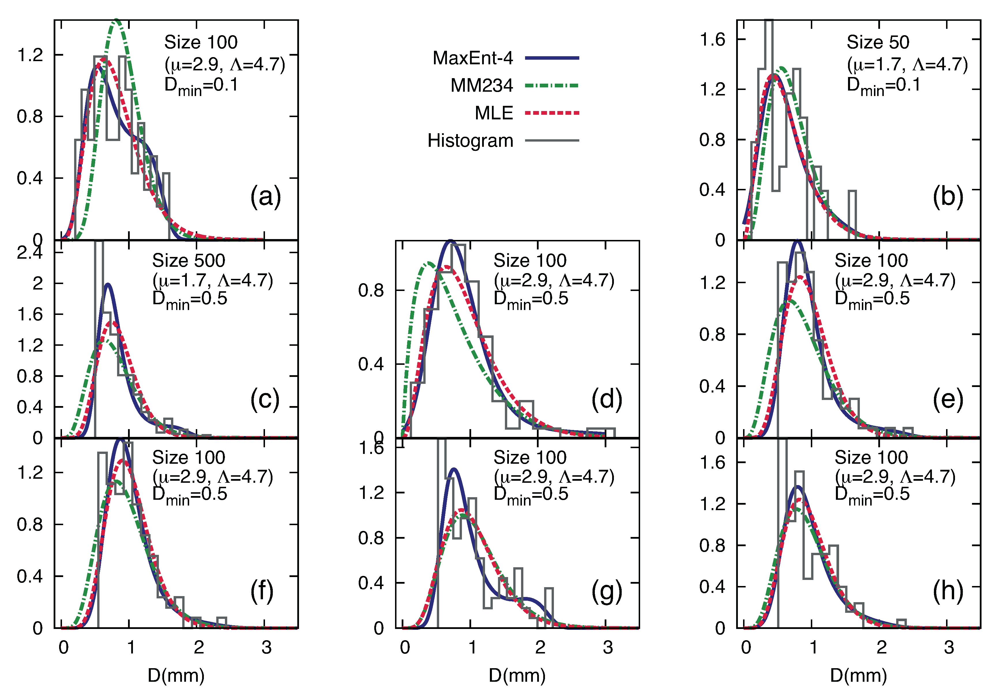
With the synthetic samples obtained as explained in Section 2.1 a binning procedure was carried out to construct histograms of 15 bins [37]. The histograms generated $\left(H_1,...,H_{15}\right)$ were normalised to $\left(h_1,...,h_{15}\right)$ to satisfy the constraint: ${\sum }_i{h}_i\delta D_i=1$. Note that $\delta D_i$ is the distance between consecutive bins which in our case is a constant value. The histograms produced by typical disdrometers are designed to follow a log-scale; the motivation to choose a constant linear-scale value is explore the robustness of MaxEnt to different binning procedures. Now the values $\left(h_1,...,h_{15}\right)$ can be compared directly with the methods explained in Section 3. An example of the histograms generated is presented in Figure 1.

Figure 1. Eight synthetic histograms together with the models obtained using the methods MLE, MM234 and MaxEnt-4 are showed. Cases with several values of $D_{min}$ and sample size are showed.

Figure 1. Eight synthetic histograms together with the models obtained using the methods MLE, MM234 and MaxEnt-4 are showed. Cases with several values of $D_{min}$ and sample size are showed.

For all histograms of each scenario, the measure $d_a\left[0\right]$ was calculated for each of the methods shown in the previous section. The measure $d_a\left[0\right]$ has numerical values that depend on the histogram, especially for samples with small number of drops. For this reason the direct comparison of the $d_a\left[0\right]$ values for two different histograms is a less valuable tool than the comparison of $d_a\left[0\right]$ for different methods but the same histogram [38]. For these reasons, we study the following measures: (1) the number of times each method reports the lowest values of $d_a\left[0\right]$ of all methods, and (2) the relative values $d_a\left[0\right]/d_a^{MLE}\left[0\right]$, taking MLE as a reference. By studying a significant number of histograms for each scenario we will be able to show the systematic behaviours of different methods. For the 50 different scenarios studied 50 histograms were enough to highlight comparative properties between methods [39].

Table 2 illustrates the results obtained for all scenarios studied with a fixed category. The number of cases in which each method produces the best value of $d_a\left[0\right]$ is shown together with the number of times in which each method improves the MLE. Illustrative examples of the histograms are present in Figure 1 comparing the methods MLE, MM234 and MaxEnt-4. Figure 2 compares MaxEnt-4, MaxEnt-6 and MaxEnt-8 for the same histograms. Figure 3 shows significance of $D_{min}$ and the number of drops, again using MLE as a reference. Finally, the relatives values, $d_a\left[0\right]/d_a^{MLE}\left[0\right]$, are shown in Figure 4 for 4 different scenarios.

Table 2. For the category “Moderate” (see Table 1) used for synthetic generation: The number of times that each method produces lower levels of difference with respect to the histogram, as measured with $d_a\left[0\right]$. Between parentheses is the number of cases in which a method has a value of $d_a\left[0\right]$ lower than that value derived under MLE. The symbol (*) indicates the presence of a sample without convergence (see the main text). As explained in the main text, size represents the number of drops of each histogram, for each scenario (μ, λ, $D_{min}$ and Size) 50 histograms were generated.

Scenario			Methods of Modelling
Rain Category	$D_{min}$	Size	MLE	MM234		MaxEnt-3		MaxEnt-4		MaxEnt-6		MaxEnt-8
Moderate	0.0	50	0	0	(10)	0	(22)	1	(35)	6	(45)	(*)43 (50)
		100	1	0	(7)	0	(17)	1	(24)	9	(39)	39 (50)
		200	3	0	(5)	1	(11)	4	(21)	11	(32)	31 (50)
		500	3	0	(6)	0	(4)	0	(11)	11	(36)	36 (50)
	0.1	50	1	0	(5)	1	(17)	1	(24)	8	(41)	39 (50)
		100	1	0	(4)	1	(12)	3	(31)	12	(43)	33 (50)
		200	3	0	(3)	0	(6)	1	(19)	7	(33)	39 (50)
		500	7	0	(1)	0	(4)	4	(15)	2	(25)	37 (50)
	0.3	100	1	0	(16)	0	(3)	1	(23)	4	(40)	44 (50)
	0.5	50	0	1	(25)	0	(0)	1	(31)	14	(48)	(*)34 (50)
		100	0	0	(35)	0	(1)	0	(36)	7	(46)	(*)42 (50)
		200	0	0	(37)	0	(0)	0	(29)	3	(46)	47 (50)
		500	0	0	(45)	0	(0)	0	(32)	0	(48)	50 (50)

Table 2. For the category “Moderate” (see Table 1) used for synthetic generation: The number of times that each method produces lower levels of difference with respect to the histogram, as measured with $d_a\left[0\right]$. Between parentheses is the number of cases in which a method has a value of $d_a\left[0\right]$ lower than that value derived under MLE. The symbol (*) indicates the presence of a sample without convergence (see the main text). As explained in the main text, size represents the number of drops of each histogram, for each scenario (μ, λ, $D_{min}$ and Size) 50 histograms were generated.

Scenario			Methods of Modelling
Rain Category	$D_{min}$	Size	MLE	MM234		MaxEnt-3		MaxEnt-4		MaxEnt-6		MaxEnt-8
Moderate	0.0	50	0	0	(10)	0	(22)	1	(35)	6	(45)	(*)43 (50)
		100	1	0	(7)	0	(17)	1	(24)	9	(39)	39 (50)
		200	3	0	(5)	1	(11)	4	(21)	11	(32)	31 (50)
		500	3	0	(6)	0	(4)	0	(11)	11	(36)	36 (50)
	0.1	50	1	0	(5)	1	(17)	1	(24)	8	(41)	39 (50)
		100	1	0	(4)	1	(12)	3	(31)	12	(43)	33 (50)
		200	3	0	(3)	0	(6)	1	(19)	7	(33)	39 (50)
		500	7	0	(1)	0	(4)	4	(15)	2	(25)	37 (50)
	0.3	100	1	0	(16)	0	(3)	1	(23)	4	(40)	44 (50)
	0.5	50	0	1	(25)	0	(0)	1	(31)	14	(48)	(*)34 (50)
		100	0	0	(35)	0	(1)	0	(36)	7	(46)	(*)42 (50)
		200	0	0	(37)	0	(0)	0	(29)	3	(46)	47 (50)
		500	0	0	(45)	0	(0)	0	(32)	0	(48)	50 (50)

The drawback of MaxEnt respect to other methods in the synthetic cases relates to the numerical solution of the problem. With our convergence parameters the system always solved for MaxEnt-3 and MaxEnt-4. Meanwhile, only 3 cases out of 2,500 histograms evaluated failed to achieve convergence for MaxEnt-6. For MaxEnt-8 around 1% of the samples either required further iterations or simply did not converge under the algorithm. These problems of convergence are present in the more challenging samples involving few drops and higher $D_{min}$. It important to note that while MM234 and MLE always provide solutions to the problem, these solutions may not faithfully represent the underlying histogram. On these cases MaxEnt-4 and MaxEnt-6 provide better approximations to the problem.

From 80% of the entire set of 2,500 histograms MaxEnt-8 produces lower values of $d_a\left[0\right]$. This fact makes logical sense, as a larger set of free parameters allow a more accurate representation of the histogram. For 68% of the scenarios with $D_{min}=0$, MaxEnt-8 produces lower values of $d_a\left[0\right]$, while for the scenarios with $D_{min}=0.5$ the percentage is 85%. These data show that for lower values of $D_{min}$ (with large values of the size) the histograms are well described by MaxEnt-4 and MLE. If MaxEnt-8 is excluded from the comparison, MaxEnt-6 produces the best performance in the 63% of the total number of histograms. Comparing only MLE, MM234 and MaxEnt-4, the latter one produces lower values $d_a\left[0\right]$ for 40% of the scenarios of the entire set. This shows how MaxEnt is a progressive method of incorporating information, while the results for MaxEnt-4 are interesting because a more realistic RDSD using a fixed distribution function would need add model errors and a direct consequence is a decrease in the performance of MLE and MM234.

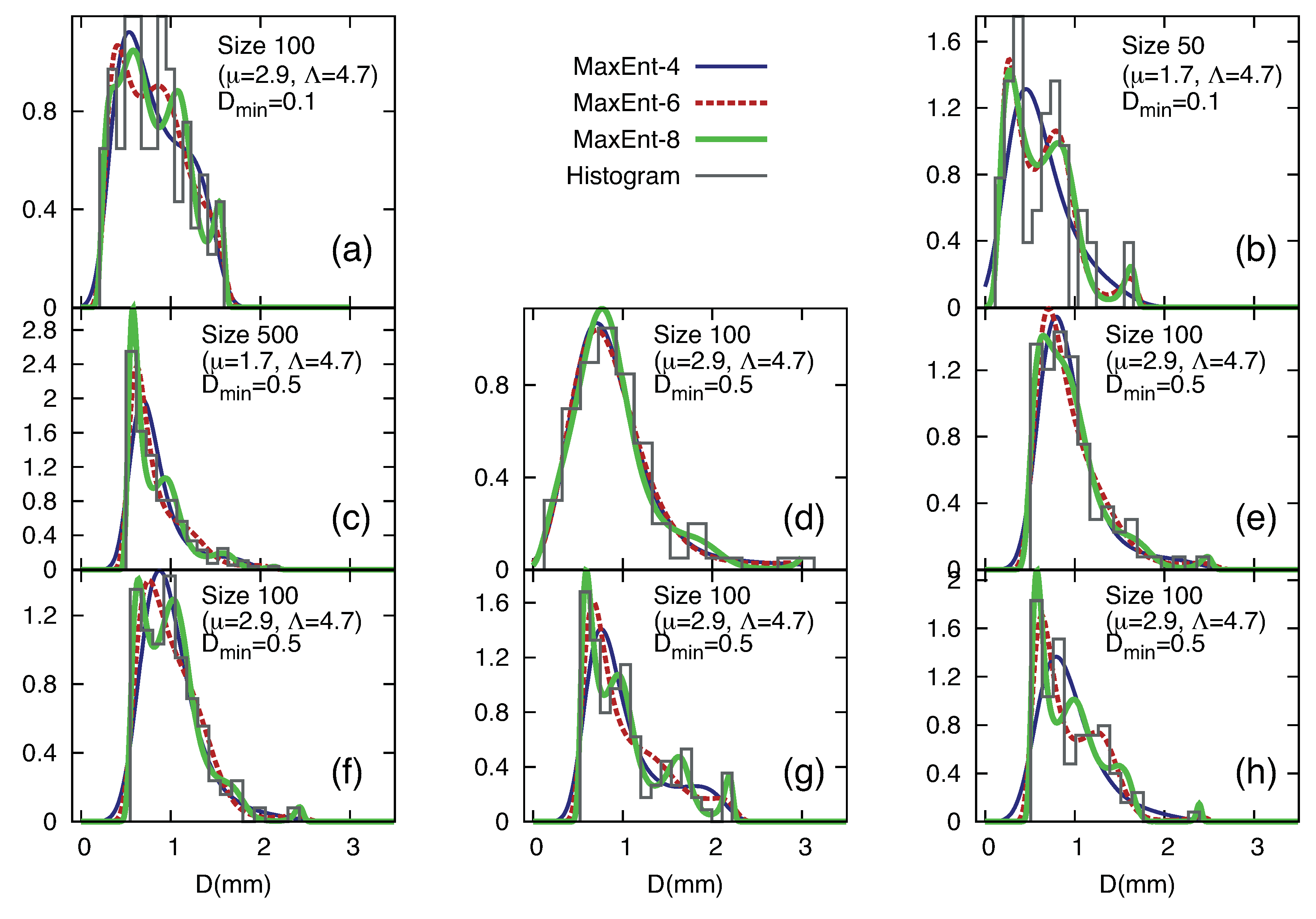
In the 15% of the total histograms analysed MaxEnt-6 produces lower values of $d_a\left[0\right]$ than any other method. This, together with the generally similar values of $d_a\left[0\right]$ for MaxEnt-6 and MaxEnt-8 (see Figure 4) may be interpreted to mean that the information contained in the integral rainfall parameters from the total number of drops until to the reflectivity is enough to retrieve an accurate representation of the samples. In the values of $d_a\left[0\right]$ a small dependence in the histogram binning procedure is possible, as shown in the panels (c) and (h) of Figure 2, while different binning procedures produce the same global results when the total number of histograms generated are compared.

Figure 2. Eight synthetic histograms together with the models obtained using methods MaxEnt-4, MaxEnt-6, MaxEnt-8 are showed. Cases with several values of $D_{min}$ and sample size are showed.

Figure 2. Eight synthetic histograms together with the models obtained using methods MaxEnt-4, MaxEnt-6, MaxEnt-8 are showed. Cases with several values of $D_{min}$ and sample size are showed.

MaxEnt-3 model of the RDSD, which includes the integral rainfall parameters up to the liquid water content, is a good method for small samples compared with MLE or MM234. Including just one more constraint, MaxEnt-4 obtained better results than MLE in 51% of the histograms, with suitable performance for $D_{min}\ne 0$ and versatile behaviour for samples with different number of drops.

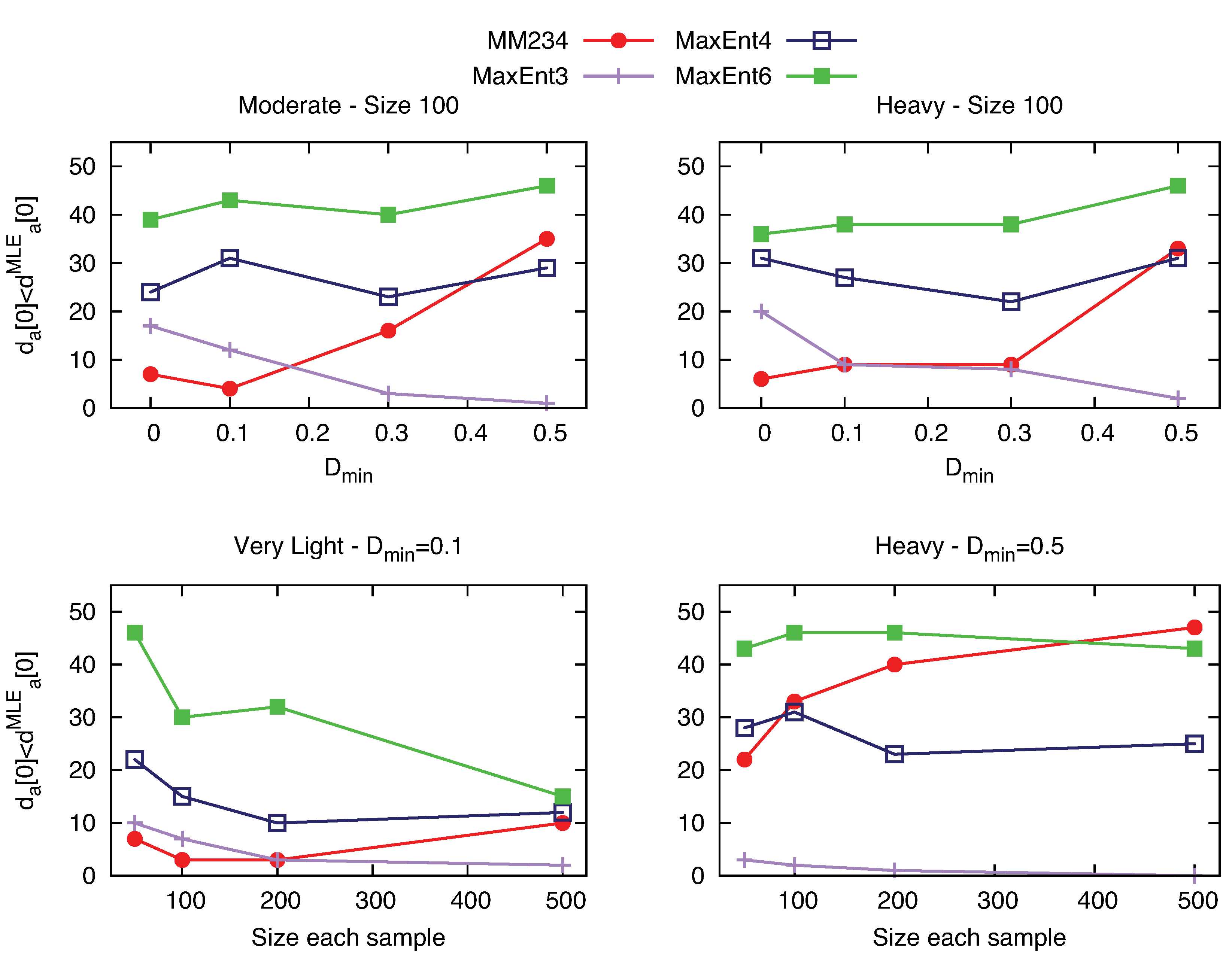
MM234 outperforms the MLE method when larger values $D_{min}$ are introduced. These drawbacks of MLE in estimating the parameters of a distribution are well known, but here the study focuses on analysing the case with the measure $d_a\left[0\right]$. This is shown in the Figure 3.

Figure 3. Number of cases in which each model reports lower value of $d_a\left[0\right]$ than MLE. Different scenarios are showed.

Figure 3. Number of cases in which each model reports lower value of $d_a\left[0\right]$ than MLE. Different scenarios are showed.

In the case of MLE, the results show that MLE optimises the model using values of the samples instead of the moments; however, the capacity of this method is strongly conditioned by the characteristics of the sample. In such situations for values of $D_{min}=0.5$, MM234 provides a better representation of the histogram; see Table 2, particularly the second column on MM234. This justifies the general preference for the method of moments over MLE. The panels (d) and (e) Figure 1 illustrate cases in which MLE outperforms MM234 for $D_{min}=0.5$ whereas for 33 cases out of 50, the result is the opposite. This shows how necessary it is to consider a large number of histograms. Finally, these results also suggest that methods of MLE applied to a truncated gamma distribution can improve compared to MM234 [29], although these methods there are not widely used [10,15]. However, from the point of view of comparing with MaxEnt a completely realistic RDSD simulation includes model errors that also decrease the capacities of MLE and MM234 for specific truncated methods, and the differences with MaxEnt may remain similar.

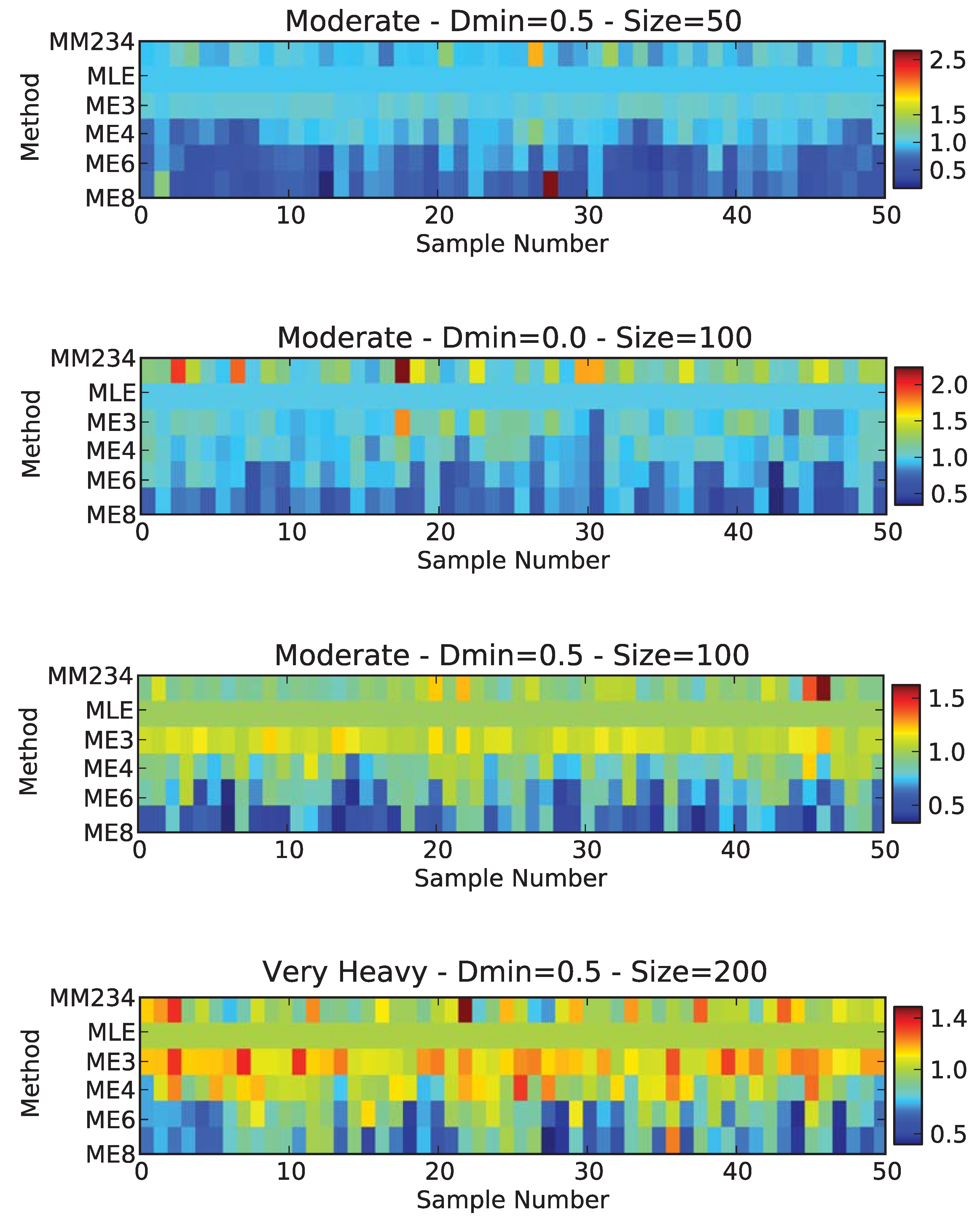
The roles of $D_{min}$ and the sample size are visually illustrated for all methods in Figure 4. It shows the progressive improvement of MaxEnt. The relative differences in $d_a\left[0\right]$ between MLE and MaxEnt-6 (or MaxEnt-8) can reach a factor of two. As noted above, with $D_{min}=0.5$, MM234 generally improves the estimate of MLE but lacks consistency. However, due to sampling variability regarding the presence of larger drops in some samples MM234 may lose part of the information present in the histogram; see Figure 1 subplot (d).

Figure 4. Values of $d_a\left[0\right]$ relative to the value for the MLE method, $d_a\left[0\right]/d_a^{MLE}\left[0\right]$. Cases with several values of $D_{min}$ and sample size are shown. In first subplot, the sample 28 is a case of non-convergence.

Figure 4. Values of $d_a\left[0\right]$ relative to the value for the MLE method, $d_a\left[0\right]/d_a^{MLE}\left[0\right]$. Cases with several values of $D_{min}$ and sample size are shown. In first subplot, the sample 28 is a case of non-convergence.

A different estimate of the advantages of each method may be obtained by comparing $F_X^{\left(1\right)}$ and $F_X^{\left(2\right)}$. In our cases, it is interesting to compare the capacities of the different methods to represent different integral rainfall parameters: the mean diameter is ${\Phi }_1$, the mean mass diameter is the quotient ${\Phi }_4/{\Phi }_3$, and the reflectivity is related to ${\Phi }_6$, so we will compare all values from ${\Phi }_1$ until ${\Phi }_6$. We ask two main questions, (1) What is the ability of each method to reproduce given values of empiric integral rainfall parameters? For this objective, it is useful to consider $F_X^{\left(1\right)}$. (2) What are the differences when we compare the integral rainfall parameters obtained from a hypothetical gamma distribution function?

The results are shown in Table 3 and Table 4. The first shows how MaxEnt-6 represents a model whose expected values for the integral rainfall parameters are the empirical values. It also shows how MaxEnt-4 gives excellent results for integral rainfall parameters related to the kinetic energy of drops, ${\Phi }_5$, and to the reflectivity ${\Phi }_6$, without constraints on the probability density function as in MaxEnt-6. This shows how MaxEnt-4 may be a valuable tool to study Z-R relations based on empirical values of rainfall. It also shows another interesting result: the information contained in the integral parameters up to the rainfall fixes all of the remaining integral parameters.

Table 3. Fractional Error $F^{\left(1\right)}$ for the Integral Parameters. The field with the character "-" means that the error is lower than $0.0001$, typically is ${10}^{-5}$ to ${10}^{-7}$.

Scenario			Method	${\text{F}}^{\left(1\right)}$
Rain Category	$D_{min}$	Size	Modelling	${\Phi }_1$	${\Phi }_2$	${\Phi }_3$	${\Phi }_4$	${\Phi }_5$	${\Phi }_6$
Very Heavy	0.1	100	MLE	-	0.033	0.122	0.260	0.418	0.571
			MM234	0.088	0.105	0.109	0.117	0.125	0.123
			MaxEnt-4	-	-	-	-	0.004	0.018
			MaxEnt-6	-	-	-	-	-	-
Moderate	0.0	500	MLE	-	0.013	0.050	0.109	0.180	0.250
			MM234	0.048	0.057	0.057	0.057	0.054	0.041
			MaxEnt-4	-	-	-	-	0.011	0.045
			MaxEnt-6	-	-	-	-	-	-
Moderate	0.5	50	MLE	-	0.037	0.133	0.271	0.415	0.539
			MM234	0.052	0.055	0.055	0.055	0.034	0.035
			MaxEnt-4	-	-	-	-	0.003	0.012
			MaxEnt-6	-	-	-	-	-	-
Very Light	0.5	200	MLE	-	0.053	0.208	0.457	0.744	1.012
			MM234	0.230	0.283	0.283	0.283	0.289	0.281
			MaxEnt-4	-	-	-	-	0.008	0.035
			MaxEnt-6	-	-	-	-	-	-

Table 3. Fractional Error $F^{\left(1\right)}$ for the Integral Parameters. The field with the character "-" means that the error is lower than $0.0001$, typically is ${10}^{-5}$ to ${10}^{-7}$.

Scenario			Method	${\text{F}}^{\left(1\right)}$
Rain Category	$D_{min}$	Size	Modelling	${\Phi }_1$	${\Phi }_2$	${\Phi }_3$	${\Phi }_4$	${\Phi }_5$	${\Phi }_6$
Very Heavy	0.1	100	MLE	-	0.033	0.122	0.260	0.418	0.571
			MM234	0.088	0.105	0.109	0.117	0.125	0.123
			MaxEnt-4	-	-	-	-	0.004	0.018
			MaxEnt-6	-	-	-	-	-	-
Moderate	0.0	500	MLE	-	0.013	0.050	0.109	0.180	0.250
			MM234	0.048	0.057	0.057	0.057	0.054	0.041
			MaxEnt-4	-	-	-	-	0.011	0.045
			MaxEnt-6	-	-	-	-	-	-
Moderate	0.5	50	MLE	-	0.037	0.133	0.271	0.415	0.539
			MM234	0.052	0.055	0.055	0.055	0.034	0.035
			MaxEnt-4	-	-	-	-	0.003	0.012
			MaxEnt-6	-	-	-	-	-	-
Very Light	0.5	200	MLE	-	0.053	0.208	0.457	0.744	1.012
			MM234	0.230	0.283	0.283	0.283	0.289	0.281
			MaxEnt-4	-	-	-	-	0.008	0.035
			MaxEnt-6	-	-	-	-	-	-

In the results for $F_X^{\left(2\right)}$, larger differences between MaxEnt and MLE or MM234 were expected, as the functional form for N(D) is different in our application of MaxEnt, however, the actual results are similar to those of MM234 and, depending on the scenario, could be better or worse than MLE, but always with reasonable values. This means that even in the hypothetical cases in which the underlying distribution is a gamma distribution function MaxEnt-4 is a useful model. Obviously if the gamma distribution is considered to be the real distribution function, then this hypothesis may be included in the maximum entropy formalism as explained above.

Table 4. Fractional Error $F^{\left(2\right)}$ for the Integral Parameters.

Scenario			Method	${\text{F}}^{\left(2\right)}$
Rain Category	$D_{min}$	Size	Modelling	${\Phi }_1$	${\Phi }_2$	${\Phi }_3$	${\Phi }_4$	${\Phi }_5$	${\Phi }_6$
Very Heavy	0.1	100	MLE	0.023	0.048	0.076	0.105	0.135	0.166
			MM234	0.065	0.027	0.091	0.282	0.544	0.880
			MaxEnt-4	0.023	0.083	0.212	0.425	0.713	1.047
			MaxEnt-6	0.023	0.083	0.212	0.425	0.719	1.075
Moderate	0.0	500	MLE	0.016	0.050	0.097	0.150	0.208	0.269
			MM234	0.063	0.093	0.103	0.099	0.085	0.062
			MaxEnt-4	0.016	0.038	0.048	0.044	0.041	0.066
			MaxEnt-6	0.016	0.038	0.048	0.044	0.031	0.022
Moderate	0.5	50	MLE	0.032	0.147	0.436	0.749	1.034	1.268
			MM234	0.020	0.164	0.372	0.600	0.821	1.021
			MaxEnt-4	0.032	0.113	0.326	0.562	0.804	1.041
			MaxEnt-6	0.032	0.113	0.326	0.562	0.802	1.036
Very Light	0.5	200	MLE	0.937	1.514	1.655	1.432	0.978	0.428
			MM234	0.599	1.098	1.502	1.818	2.056	2.225
			MaxEnt-4	0.937	1.608	2.079	2.448	2.723	2.829
			MaxEnt-6	0.937	1.608	2.079	2.448	2.742	2.914

Table 4. Fractional Error $F^{\left(2\right)}$ for the Integral Parameters.

Scenario			Method	${\text{F}}^{\left(2\right)}$
Rain Category	$D_{min}$	Size	Modelling	${\Phi }_1$	${\Phi }_2$	${\Phi }_3$	${\Phi }_4$	${\Phi }_5$	${\Phi }_6$
Very Heavy	0.1	100	MLE	0.023	0.048	0.076	0.105	0.135	0.166
			MM234	0.065	0.027	0.091	0.282	0.544	0.880
			MaxEnt-4	0.023	0.083	0.212	0.425	0.713	1.047
			MaxEnt-6	0.023	0.083	0.212	0.425	0.719	1.075
Moderate	0.0	500	MLE	0.016	0.050	0.097	0.150	0.208	0.269
			MM234	0.063	0.093	0.103	0.099	0.085	0.062
			MaxEnt-4	0.016	0.038	0.048	0.044	0.041	0.066
			MaxEnt-6	0.016	0.038	0.048	0.044	0.031	0.022
Moderate	0.5	50	MLE	0.032	0.147	0.436	0.749	1.034	1.268
			MM234	0.020	0.164	0.372	0.600	0.821	1.021
			MaxEnt-4	0.032	0.113	0.326	0.562	0.804	1.041
			MaxEnt-6	0.032	0.113	0.326	0.562	0.802	1.036
Very Light	0.5	200	MLE	0.937	1.514	1.655	1.432	0.978	0.428
			MM234	0.599	1.098	1.502	1.818	2.056	2.225
			MaxEnt-4	0.937	1.608	2.079	2.448	2.723	2.829
			MaxEnt-6	0.937	1.608	2.079	2.448	2.742	2.914

4.2. Analysis of Experimental Measurements

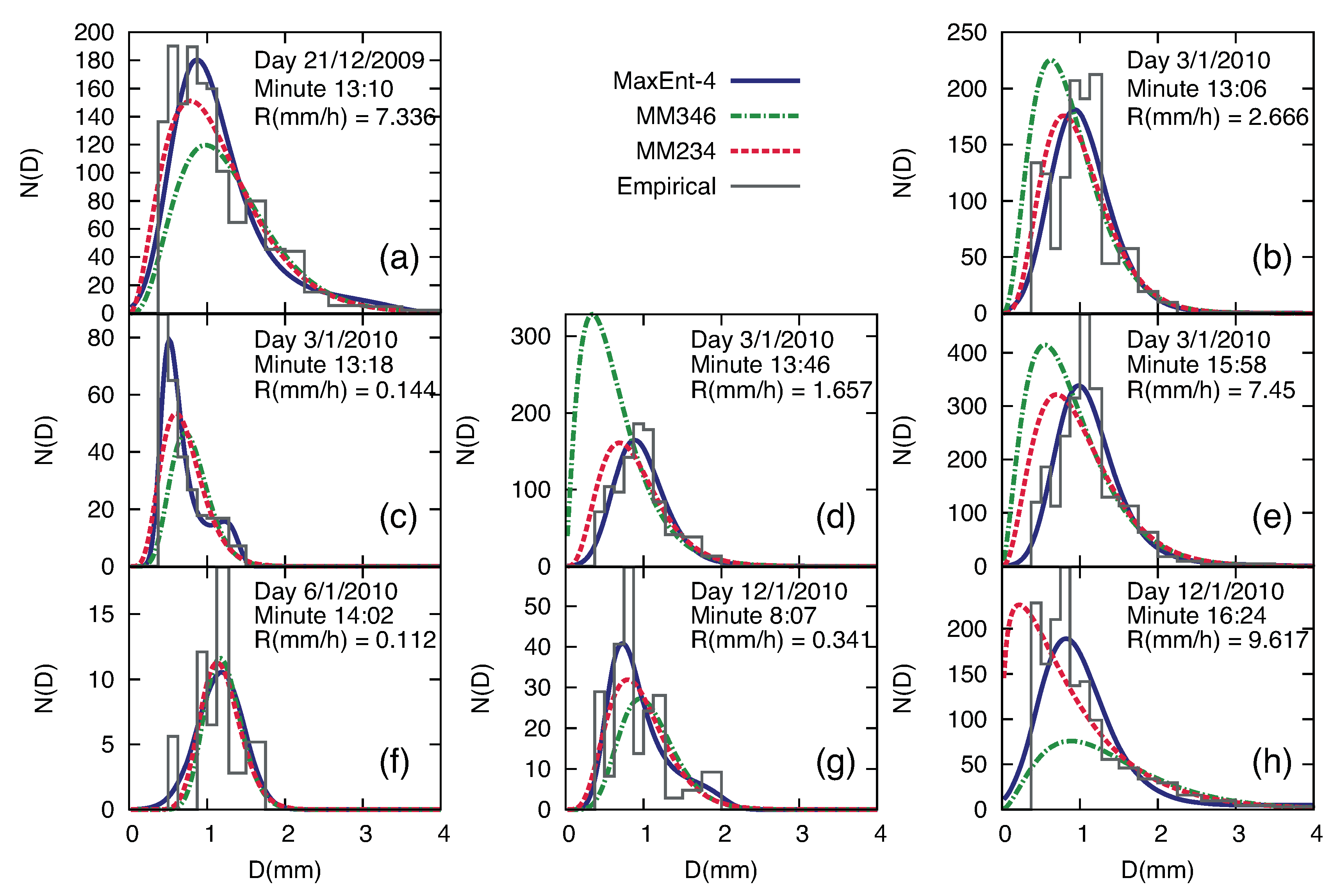
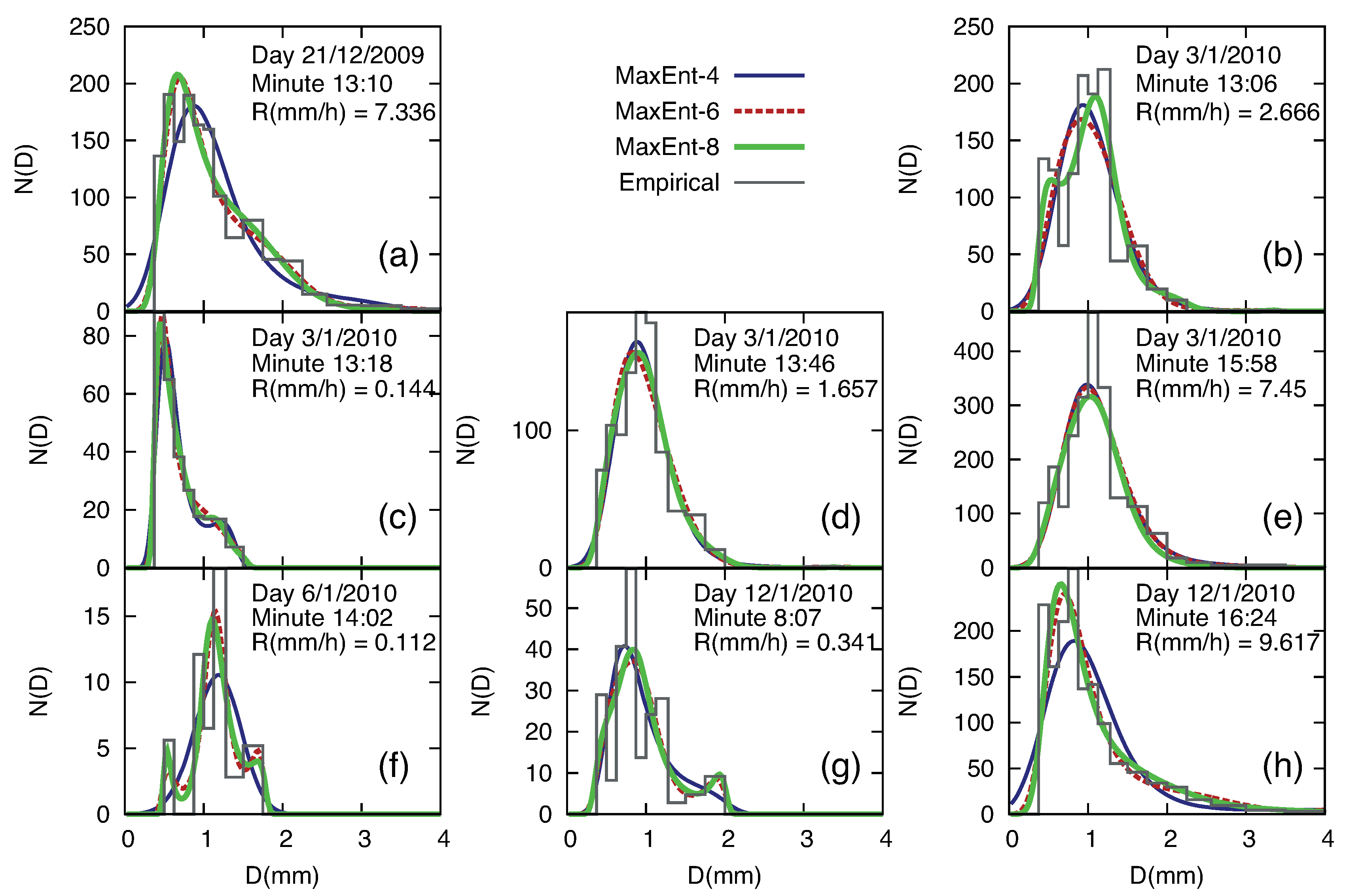
Experimental histograms are shown in Figure 5 and Figure 6 for the four different rain events. The general results are analogous to the synthetic histograms. Subplots (f) and (g) of Figure 6 show that MaxEnt-6 and MaxEnt-8 can model adequately several peaks. MaxEnt-6 is able to model cases with a second peak with larger drops (typical multimodal cases), while MaxEnt-8 may model cases with several peaks as well as small drops with low rainfall intensity. The Figure 5 illustrates how—for subplots (d) and (h)—MM346 fails to provide a reasonable prediction for the smallest drops and, consequently, underestimates the total number of drops. The method is designed to represent experimental liquid water content $M_3$ and reflectivity $M_6$. However, when comparing the subplots (a) and (e), both with similar amount of rainfall, the presence of a few large drops results in an uncontrolled prediction for smaller drops. MM234 shows more stability and results in a more systematic representation of the histogram, while this representation is improved using the MaxEnt methods. The comparison of subplots (a) and (b) is illustrative of the role of larger drops in rainfall.

Figure 5. Eight Experimental histograms together with the models obtained using different methods are showed. The value of Rainfall as calculated from the sample is showed for comparative. MM234, MM346 and MaxEnt-4 are showed.

Figure 5. Eight Experimental histograms together with the models obtained using different methods are showed. The value of Rainfall as calculated from the sample is showed for comparative. MM234, MM346 and MaxEnt-4 are showed.

Figure 6. Eight Experimental histograms together with the models obtained using different methods are showed. The value of Rainfall as calculated from the sample is showed for comparative. Maximum Entropy models are showed.

Figure 6. Eight Experimental histograms together with the models obtained using different methods are showed. The value of Rainfall as calculated from the sample is showed for comparative. Maximum Entropy models are showed.

These facts can be appreciated in Figure 7, where measure $d\left[0\right]$ is applied. The value of $lo{g}_{10}\left|d\left[0\right]\right|$ is shown for the four different rain events. MM346 systematically results in larger values, though similar in magnitude to MM234, while the results of MaxEnt are always lower. In fact, MM346 in many cases provides a value that is too high or too low with respect to the total number of drops. This happen occurs for MM234, though less frequently. On the other hand MaxEnt-4 without capturing all details of the histogram is a good representation of it.

Figure 7. Comparison of $lo{g}_{10}\left|d\left[0\right]\right|$ for the four episodes of rain analyzed and for all methods used in Experimental Modeling.

Figure 7. Comparison of $lo{g}_{10}\left|d\left[0\right]\right|$ for the four episodes of rain analyzed and for all methods used in Experimental Modeling.

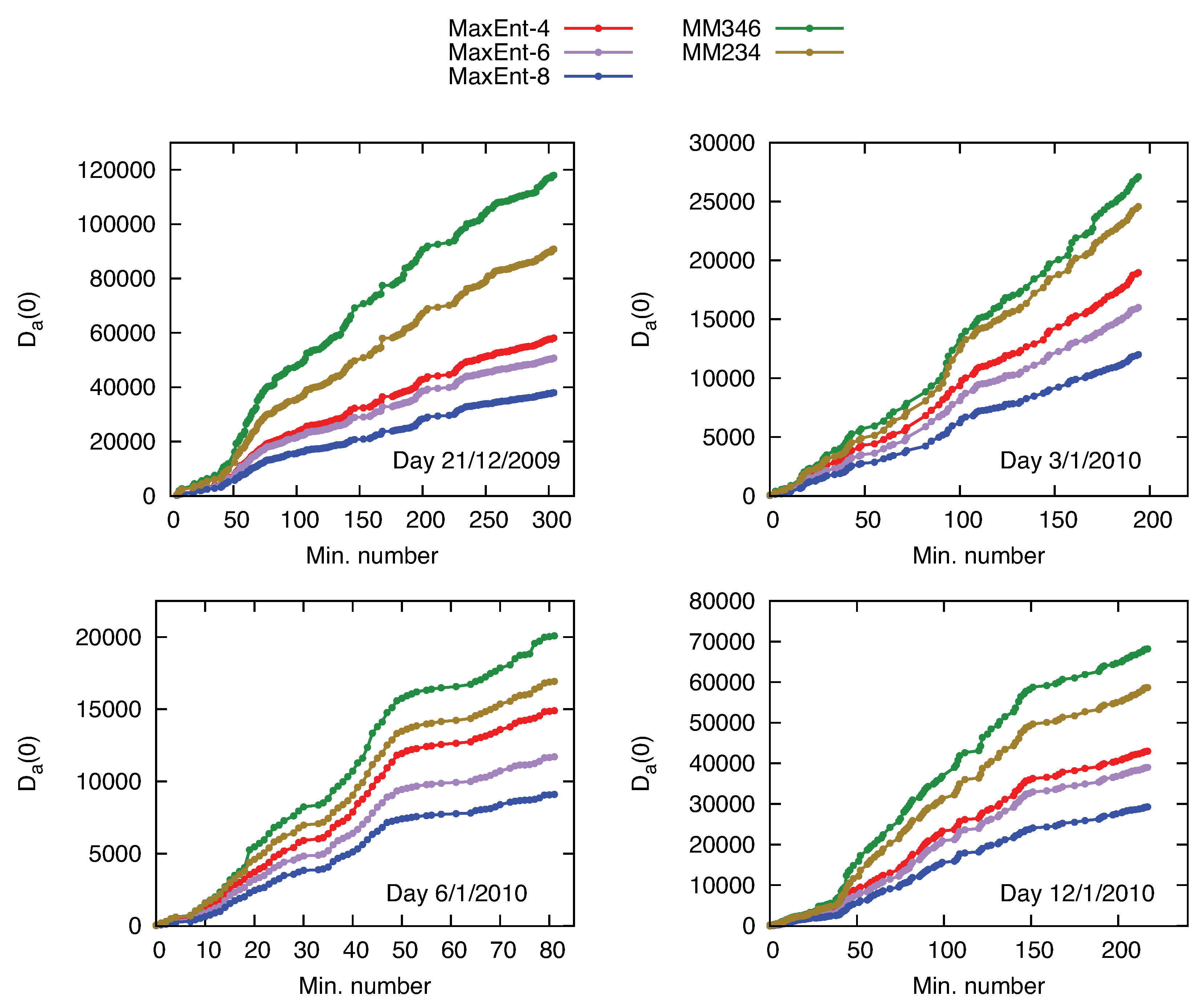
As a result of the behaviour previously noted, the accumulation of differences, $D_a\left[0\right]$, is an increasing monotonic function with different rates. It is larger under the method of moments that under the MaxEnt methods. However, Figure 8 shows a correlation between all methods, all of which allow discriminate periods of larger relative rates of increase, related presumably with intrinsic properties of the rainfall process.

Looking to the experimental dataset, findings on convergence are similar to the synthetic analysis. However, a careful comparison allows us to discriminate two cases of convergence problems. Some histograms with fewer that 10 drops required more effective algorithms to solve the system and maximise of the entropy functional. As noted before, problems related to a small number of drops are present in all methods, and for practical purposes, some authors preprocess data so that data with fewer than 10 drops are classified as noise. For those analyses the algorithm applied to retrieve the RDSD using MaxEnt is simple.

Figure 8. Comparison of $D_a\left[0\right]$ for the four episodes of rain analyzed and for all methods used in Experimental Modeling.

Figure 8. Comparison of $D_a\left[0\right]$ for the four episodes of rain analyzed and for all methods used in Experimental Modeling.

A previous study on sprays [40] reported situations in which this algorithm fails to convergence instead reaches a narrow, non-physical fixed peak. Both situations explain why in around a 5–7% of the cases do not convergence for MaxEnt-8 (that is, given the reasonable difference within the data and a limited number of iterations), though convergence is better under MaxEnt-6. For the cases reported here, it may be possible improve the Newton-Raphson algorithm [41] or avoid using it by instead using more recently introduced algorithms [42].

In our comparative study with other methods, see Figure 7 and Figure 8, the cases with fewest number of drops that did not converge are not considered as in the previous methods, because they cannot be used to provide a convenient solution. Meanwhile the case of a narrow, large peak is easily detected as indicating higher differences within histogram (or integral parameters such as rainfall or reflectivity). Figure 7 and Figure 8 do not include histograms in which any of the methods show a value of $d_a\left[0\right]$ higher than the prescribed threshold. The criterion to determinate this threshold is aimed at eliminating similar number of samples with high values of $d_a\left[0\right]$ under method of moments as the number eliminated for non-convergence under MaxEnt-8 method. The resulting, an improved algorithm could provide higher differences under MaxEnt methods. In other words, the threshold is selected to prune cases of non-convergence under MaxEnt-8 as well as the cases of null representability with respect to the histograms generated under the method of moments.

5. Discussion

The maximum entropy modelling applied to RDSDs outperforms other analysed methods for both synthetic and experimental datasets, in terms of providing the empirical values of the integral rainfall parameters and reproducing a given histogram.

In those cases where there is a sufficient amount of drops and measurements of all sizes, the MLE will satisfactory represent a sample. However, whenever these conditions are not true, the method of moments can improve the predictions of MLE.

On the other hand, the MaxEnt method shows a systematic and progressive approximation of the empirical information; while MaxEnt-3 is a coarse representation of the histogram, MaxEnt-4 and MaxEnt-6 achieve a gradual improvement by simply incorporating more information. The only drawback of MaxEnt method are the occasional difficulties related to convergence with the exposed simple algorithm under the MaxEnt-8 model; therefore, MaxEnt-4 or MaxEnt-6 are reliable models for RDSD in the majority of the cases. The first is a general valuable model, the latter is more useful to study multimodal cases.

In the synthetic case, we tested the methods with an underlying hypothetical distribution. However in the experimental case, model errors appear, decreasing the performance when using traditional methods. In contrast, MaxEnt provides less biased probability density function which fulfills a given a set of constraints imposed by empirical information. Thus, the study of the variability of RDSD then does not rely on the capacity of a prefixed functional form to represent the RDSD for all different cases. Rather, it focuses on the physical and empirical meaningful selection of constraints. Meanwhile, the analysis of the values of λ retrieved by MaxEnt provided the necessary information to develop a deeper understanding of the questions related with the RDSD.

This opens the possibility of improving the predictions of precipitation in two different aspects; the first requires the incorporation of a more physical parametrisation of RDSD to the numerical weather prediction models, while the second requires a new method of analysis and prediction of ZR relations, which should prove useful for ground and space-borne meteorological radars.

6. Conclusions

The formulation of statistical mechanics as proposed by Jaynes [16] is conceptualised as a general inference method resulting in the maximum entropy principle, which allows to understand physical systems of stochastic origin and formulate more objective and systematic models. This formulation of statistical mechanics, and its underlying entropy concept have been applied to many fields in earth sciences [43], from problems similar to the presented in this paper to problems related to reformulations of the MaxEnt as a maximum entropy production postulate; for more details, see [44] and the reference there contained.

Under the maximum entropy principle the probability density function represents the best guess according to available knowledge. The method also has a physical significance when used to understand the processes of the earth’s physics. This paper provides an application to a real problem that is present in the microphysics of precipitation resulting in a physically based method rather than merely experimental fit.

References and Notes

- Rosenfeld, D.; Lohmann, U.; Raga, G.B.; O’Dowd, C.D.; Kulmala, M.; Fuzzi, S.; Reissell, A.; Andreae, M.O. Flood or Drought: How Do Aerosols Affect Precipitation? Science 2008, 321, 1309. [Google Scholar] [CrossRef] [PubMed]
- Tokay, A.; Kruger, A.; Krajewski, W.F. Comparison of Drop Size Distribution Measurements by Impact and Optical Disdrometers. J. Appl. Meteor. 1996, 40, 2083–2097. [Google Scholar] [CrossRef]
- Krajewski, W.F.; Kruger, A.; Caracciolo, C.; Golé, R.; Barthes, L.; Creutin, J.D.; Delahaye, J.Y.; Nikolopoulus, E.I.; Odgen, F.; Vison, J.P. DEVEX-disdrometer evaluation experiment: Basic results and implications for hydrological studies. Adv. Water Res. 2006, 26, 311–325. [Google Scholar] [CrossRef]
- Marshall, J.S.; Palmer, W.M.K. The distribution of raindrops with size. J. Meteor. 1948, 5, 165–166. [Google Scholar] [CrossRef]
- Feingold, G.; Levin, Z. The log-normal fit to raindrop spectra from frontal convective clouds in Israel. J. Appl. Meteor. 1986, 25, 1346–1363. [Google Scholar] [CrossRef]
- Feingold, G.; Levin, Z. The log-normal size distribution of raindrops: Application to differential reflectivity measurements of rainfall (ZDR). J. Atmos. Oceanic Technol. 1987, 4, 377–382. [Google Scholar] [CrossRef]
- Ulbrich, C.W. Natural variations in the analytical form of the raindrop size distribution. J. Climate Appl. Meteor. 1983, 22, 1764–1775. [Google Scholar] [CrossRef]
- Sauvageot, H.; Koffi, M. Multimodal Raindrop Size Distributions. J. Atmos. Sci. 2000, 57, 2480–2492. [Google Scholar] [CrossRef]
- Radhakrishna, B.; Narayana, T.R. Statistical Characteristics of Multipeak Raindrop Size Distributions at the Surface and Aloft in Different Rain Regimes. Mon. Wea. Rev. 2009, 137, 3501–3518. [Google Scholar] [CrossRef]
- Cao, Q.; Zhang, G. Errors in Estimating Raindrop Size Distribution Parameters Employing Disdrometer and Simulated Raindrop Spectra. J. Appl. Meteor. Climatol. 2009, 48, 406–425. [Google Scholar] [CrossRef]
- Sempere-Torres, D.; Porrá, J.M.; Creutin, J.M. Experimental evidence of a general description for raindrop size distribution properties. J. Geophys. Res. 1998, 103, 1785–1797. [Google Scholar] [CrossRef]
- Lee, G.; Zawadzki, I.; Szyrmer, W.; Sempere-Torres, D.; Uilenhoet, R. A General Approach to Double-Moment Normalization of Drop Size Distributions. J. Appl. Meteor. 2004, 43, 264–281. [Google Scholar] [CrossRef]
- Testud, J.; Oury, S.; Black, R.A.; Amayenc, P.; Dou, X. The Concept of “Normalized" Distribution to Describe Raindrop Spectra: A Tool for Cloud Physics and Cloud Remote Sensing. J. Appl. Meteor. 2002, 40, 1118–1140. [Google Scholar] [CrossRef]
- Smith, P.L.; Kliche, D.V. The bias in moment estimators for parameters of drop-size distribution functions: Sampling from exponential distributions. J. Appl. Meteor. 2005, 44, 1195–1205. [Google Scholar] [CrossRef]
- Kliche, D.V.; Smith, P.L.; Johnson, R.W. L-Moment Estimators as Applied to Gamma Drop Size Distributions. J. Appl. Meteor. Climatol. 2008, 47, 3117–3130. [Google Scholar] [CrossRef]
- Jaynes, E.T. Information Theory and Statistical Physics. Phys. Rev. 1957, 106, 620–630. [Google Scholar] [CrossRef]
- Dumouchel, C. The Maximum Entropy Formalism and the Prediction of Liquid Spray Drop-Size Distribution. Entropy 2009, 11, 713–747. [Google Scholar] [CrossRef]
- Babinsky, E.; Sojka, P.E. Modeling drop size distributions. Progr. Energy Combust. Sci. 2002, 28, 303–329. [Google Scholar] [CrossRef]
- Tapiador, F.J. A Maximum Entropy Analysis of Global Monthly Series of Rainfall from Merged Satellite Data. Int. J. Remote Sens. 2007, 28, 1113–1121. [Google Scholar] [CrossRef]
- Tapiador, F.J.; Kidd, C.; Levizzani, V.; Marzano, F.S. A maximum entropy approach to satellite quantitative precipitation estimation (QPE). Int. J. Remote Sens. 2004, 25, 4629–4639. [Google Scholar] [CrossRef]
- Tapiador, F.J.; Casanova, J.L. An Algorithm for the Fusion of Images based on Jaynes Maximum Entropy Method. Int. J. Remote Sens. 2002, 23, 777–785. [Google Scholar] [CrossRef]
- Liu, Y.G.; You, L.G.; Yang, W.N.; Liu, F. On the size distribution of cloud droplets. Atmos. Res. 1995, 35, 201–216. [Google Scholar] [CrossRef]
- Liu, Y.G.; Hallett, J. On the size distribution of cloud droplets by condensation: A new conceptual model. J. Atmos. Sci. 1998, 55, 527–536. [Google Scholar] [CrossRef]
- Liu, Y.G.; Daum, P.H.; Hallett, J. A generalized Systems Theory of the effect of varying Fluctuations on cloud droplet size distributions. J. Atmos. Sci. 2002, 59, 2279–2290. [Google Scholar] [CrossRef]
- Tokay, A.; Short, D.A. Evidence from tropical raindrop spectra of the origin of rain from stratiform vs convective clouds. J. Appl. Meteor. 1996, 35, 355–371. [Google Scholar] [CrossRef]
- Brawm, D.; Upton, G. Estimation of an atmospheric gamma drop size distribution using disdrometer data. Atmos. Res. 2008, 87, 66–79. [Google Scholar] [CrossRef]
- Matsumoto, M.; Nishimura, T. Mersenne twister: A 623-dimensionally equidistributed uniform pseudo-random number generator. ACM Trans. Model. Comput. Simul. 1998, 8, 3–30. [Google Scholar] [CrossRef]
- Bringi, V.N.; Huang, G.; Chandrasekar, V.; Gorgucci, E. A methodology for estimating the parameters of a gamma raindrop size distribution model from polarimetric radar data: Application to a squall-line event from the TRMM/Brazil campaign. J. Atmos. Oceanic Technol. 2002, 19, 633–645. [Google Scholar] [CrossRef]
- Mallet, C.; Barthes, L. Estimation of Gamma Raindrop Size Distribution Parameters: Statistical Fluctuations and Estimation Errors. J. Atmos. Oceanic Technol. 2008, 26, 1572–1584. [Google Scholar] [CrossRef]
- Tapiador, F.J.; Checa, R.; de Castro, M. An experiment to measure the spatial variability of rain drop size distribution using sixteen laser disdrometers. Geophys. Res. Lett. 2010, 37, L16803. [Google Scholar] [CrossRef]
- Smith, P.L. Raindrop size distributions. Exponential or Gamma—Does the difference matter? J. Appl. Meteor. 2003, 42, 1031–1034. [Google Scholar] [CrossRef]
- Ulbrich, C.W.; Atlas, D. Rainfall microphysics and radar properties: Analysis methods for drops size spectra. J. Appl. Meteor. 1998, 37, 912–923. [Google Scholar] [CrossRef]
- Kozu, T.; Nakamura, K. Rainfall parameter estimation from dual-radar measurements combining reflectivity profile and path-integrated attenuation. J. Atmos. Oceanic Technol. 1991, 8, 259–270. [Google Scholar] [CrossRef]
- Smith, P.L.; Kliche, D.V.; Johnson, R.W. The Bias and Error Estimators for Parameters of Drop Size Distribution Functions: Sampling from Gamma Distributions. J. Appl. Meteor. Climatol. 2009, 48, 2118–2126. [Google Scholar] [CrossRef]
- Shannon, C.E. A mathematical theory of communication. Bell Syst. Tech. J. 1948, 27, 379. [Google Scholar] [CrossRef]
- Singh, V.P.; Rajagopal, A.K.; Singh, K. Derivation of some frequency distributions using the principle of maximum entropy. Adv. Water Res. 1986, 9, 91–106. [Google Scholar] [CrossRef]
- In generating the histograms, histograms of 20 bins were also computed, and, in the case of the smallest sample sizes, histograms of 10 bins were produced. Analogous general behaviour was reported in both of these cases.
- It is also possible to compare the mean value of da[0] over a large set of histograms, or to analyse the values of Da[0] for an entire precipitation event.
- This is the same number of histograms per scenario that were used in the study of [29].
- Mondal, D.; Datta, A.; Sarkar, A. Droplet size and velocity distributions in a spray from a pressure swirl atomizer: Application of maximum entropy formalism. Proc. IMechE Part C J. Mech. Eng. Sci. 2004, 218, 737–749. [Google Scholar] [CrossRef]
- Abramov, R. A practical computational framework for the multidimensional moment-constrained maximum entropy principle. J. Comp. Phys. 2006, 1, 198–209. [Google Scholar] [CrossRef]
- Abramov, R. The multidimensional moment-constrained maximum entropy problem: A BFGS algorithm with constraint scaling. J. Comp. Phys. 2009, 228, 96–108. [Google Scholar] [CrossRef]
- Tapiador, F.J. Hurricane Footprints in Global Climate Models. Entropy 2008, 10, 613–620. [Google Scholar] [CrossRef]
- Niven, R.K. Steady state of a dissipative flow-controlled system and the maximum entropy production principle. Phys. Rev. E 2009, 80, 021113–021128. [Google Scholar] [CrossRef]
- Mohammad-Djafari, A. A Matlab Program to Calculate the Maximum Entropy Distributions. Max. Entropy Bayesian Meth. 1991. arXiv:physics/0111126. [Google Scholar]
Appendix
Numerical Method for Maximise the Entropy Functional
The analytical maximisation of Equation (4) is only possible for selected sets of constrains [36], and a computational framework is needed. Here is presented the application of the classical iterative method of Newton-Raphson [45] for the numerical solution of the moment-constrained maximum entropy problem.
Non-Linear Systems of Equations
The method of Lagrange multipliers provides a strategy for finding the maxima of a function, such as Equation (4) subject to a set of constraints, such as Equation (5). In this method a new function is defined as follows,
which is the function to be maximised; then the formal solution obtained for the probability density function is given by Equation (6). With this solution the constraints are now given by,
This is a set of non-linear equations in the unknowns which must now be solved.
Numerical Solution by Newton-Raphson Method
The numerical method consists of calculating the linear approximations of around trial values of , and solving the resulting linear system iteratively. We define,
and
and the problem Equation (12) is then given by,
The Jacobian of the vector function is given by,
Then, given a initial trial, it is possible to solve the Equation (15) by the iterative method,
This system is solved for from which we drive , which becomes our new initial vector and the iterations continue until is sufficiently small, i.e., , where δ is the tolerance parameter of convergence. The system is considered solved when the difference between k-th and (k+1)-th steps in the iterative process is less than , and a fixed limitation on the maximum number of iterations was also added to the solution algorithm.
Given the values of Φ, it can be a challenge to choose a convenient value for to ascertain that the iterative process converges to the fixed point representing the maximum of the entropy functional. To avoid spurious cyclic points, small perturbations were cyclically added to the value of if the iterative process oscillated periodically around a fixed value of .
The matrix equation in (17) is solved by the method of Gauss. To update the values, in each iteration, a scaling factor is introduced to stabilise the algorithm. This scaling factor ν is selected based on the convergence process and the number of constraints, in an interval from to , then the second equation in (17) is written as .
© 2011 by the authors; licensee MDPI, Basel, Switzerland. This article is an open access article distributed under the terms and conditions of the Creative Commons Attribution license (http://creativecommons.org/licenses/by/3.0/).
Share and Cite
MDPI and ACS Style
Checa, R.; Tapiador, F.J. A Maximum Entropy Modelling of the Rain Drop Size Distribution. Entropy 2011, 13, 293-315. https://doi.org/10.3390/e13020293
AMA Style
Checa R, Tapiador FJ. A Maximum Entropy Modelling of the Rain Drop Size Distribution. Entropy. 2011; 13(2):293-315. https://doi.org/10.3390/e13020293
Chicago/Turabian StyleCheca, Ramiro, and Francisco J. Tapiador. 2011. "A Maximum Entropy Modelling of the Rain Drop Size Distribution" Entropy 13, no. 2: 293-315. https://doi.org/10.3390/e13020293