Lagrange Equations Coupled to a Thermal Equation: Mechanics as Consequence of Thermodynamics

Abstract

Following the analytic approach to thermodynamics developed by Stückelberg, we study the evolution equations of a closed thermodynamic system consisting of point particles in a fluid. We obtain a system of coupled differential equations describing the mechanical and the thermal evolution of the system. The coupling between these evolution equations is due to the action of a viscous friction term. Finally, we apply our coupled evolution equations to study the thermodynamics of an isolated system consisting of identical point particles interacting through a harmonic potential.

1. Introduction

The history and development of modern thermodynamics started during the industrialisation period and was closely related to the need to improve the efficiency of steam engines. Since the foundational work of Carnot [1] in 1824, until 1960, thermodynamics has been a phenomenological theory mainly restricted to the description of either equilibrium states or transformations relating one equilibrium state to another [2]. In essence, thermodynamics was essentially reduced to thermostatics or quasi-thermostatics.

In 1960, Stückelberg [3] reformulated thermodynamics in an axiomatic way as a truly dynamic and phenomenological theory describing the evolution of a thermodynamic system by a set of first-order differential equations. By doing so, he actually extended the existing theory of equilibrium states, or thermostatic, in order to obtain a genuine thermodynamic theory, i.e., a theory describing the evolution and the approach to equilibrium of thermodynamic systems. In his axiomatic approach, he introduced, two state functions, the “energy” and the “entropy” obeying the two fundamental laws of thermodynamics. He then derived from these two laws the equations for the time evolution of the system.

In his words, the state of a thermodynamic system is defined by a set of geometric variables and a set of thermal variables. The simplest system, which he called “system element”, is a system where one thermal variable and a set of geometric variables are sufficient to define entirely the state. The second law of thermodynamics requires the existence of a state function entropy for every system. Thus, the state of a system element is defined by the entropy and a set of geometric variables. We note that the notion of system element is analogous to the concept of point particle in mechanics. It is the building block required to develop the theory of general systems where several thermal variables are necessary to define the state.

In the present work, we essentially follow the original approach of Stückelberg [3] and apply his formalism to a closed thermodynamic system consisting of N point particles moving in a fluid. The system is thus defined by the particles and the fluid, but we assume no a priori knowledge of the fluid. It is a phenomenological approach where the theory is built upon the macroscopic description of the particles (which are the only observable objects). It is thus observed that the macroscopical mechanical variables (generalised coordinates and velocities) are not sufficient to obtain the time evolution of the system. Following the thermodynamic approach, we assume the simplest possible case where the system can be described by introducing only one more non-mechanical, or thermodynamical variable, the entropy. Applying the first and second law, we obtain a system of coupled differential equations describing the thermodynamic evolution of the system. In that system of differential equations, the coupling between the resulting Lagrange equations and the thermal equation is due to the viscous friction terms depending on the state variable.

In this phenomenological approach, the theory tells us what are the quantities that should be obtained from experiment, in particular in order to obtain typical thermodynamical properties such as the specific heat. Since we have introduced a model with only one thermal variable (the total entropy), it is not possible to derive transport properties (viscosity or thermal conductivity). To obtain such a transport theory, we would need a continuum description of the fluid (density field, entropy field, ...).

The structure of this publication is as follows. In Section 2, we briefly recall Stückelberg’s axiomatic formulation of the first and second thermodynamic laws. Section 3 is devoted to establishing the equations of evolution of a system of point particles based on the first law. In Section 4, we extend the thermodynamics of a system of point particles to include the second law. Section 5 shows how thermodynamics relates to mechanics and in particular to the Lagrange equations. Finally, in Section 6, we apply our formalism to study the thermodynamics of an isolated system consisting of identical point particles interacting through a harmonic potential, which is the simplest phenomenological model of a solid.

2. Axiomatic Formulation of the First and Second Laws

2.1. First Law

For every system Σ, there exists an extensive, scalar state function E, called energy. If the system is isolated, the energy is constant, i.e., E is a conserved observable. If the system is not isolated, then

$$\frac{dE}{dt}=P_W^{\text{ext}}\left(t\right)+P_Q^{\text{ext}}\left(t\right)+P_{\text{chem}}^{\text{ext}}\left(t\right),$$

(1)

where $P_W^{\text{ext}}\left(t\right)$ is the power due to the external forces acting on the mechanical variables of the system, $P_Q^{\text{ext}}\left(t\right)$ is the power due to the heat transfer and $P_{\text{chem}}^{\text{ext}}\left(t\right)$ is the power due to the matter transfer between the system and the exterior (see [3] p. 26 and [4] p. 221).

The system is said to be “closed” if there is no exchange of matter, i.e., $P_{\text{chem}}^{\text{ext}}\left(t\right)=0$ ; it is said “adiabatically closed” if it is closed and there is no heat exchange, i.e., $P_{\text{chem}}^{\text{ext}}\left(t\right)=0$ and $P_Q^{\text{ext}}\left(t\right)=0$. It is said isolated if it is adiabatically closed and there is no mechanical power exchange, i.e., $P_{\text{chem}}^{\text{ext}}\left(t\right)=0$, $P_Q^{\text{ext}}\left(t\right)=0$ and $P_W^{\text{ext}}\left(t\right)=0$, in which case the energy E is a constant.

2.2. Second Law

For every system Σ, there exists an extensive, scalar state function S, called entropy, which obeys the following two conditions (see [3] p. 23) :

(a)

Evolution Part :

If the system is adiabatically closed, the entropy S is a non-decreasing function with respect to time, i.e.,

$$\frac{dS}{dt}=I\left(t\right)⩾0,$$

(2)

where $I\left(t\right)$ is the entropy production rate of the system accounting for the irreversibility of internal thermal processes.

(b)

Equilibrium Part :

If the system is isolated, as time tends to infinity (i.e., $t\to +\infty$) the entropy tends towards a finite local maximum [5], compatible with the constraints (internal walls and isolation conditions), i.e.,

$$\underset{t\to +\infty }{lim}S\left(t\right)=\underset{\rho \text{compatible}}{max}S\left[\rho \right],$$

(3)

where ρ compatible denotes a thermodynamic state compatible with the constraints.

3. System of Point Particles: First Law

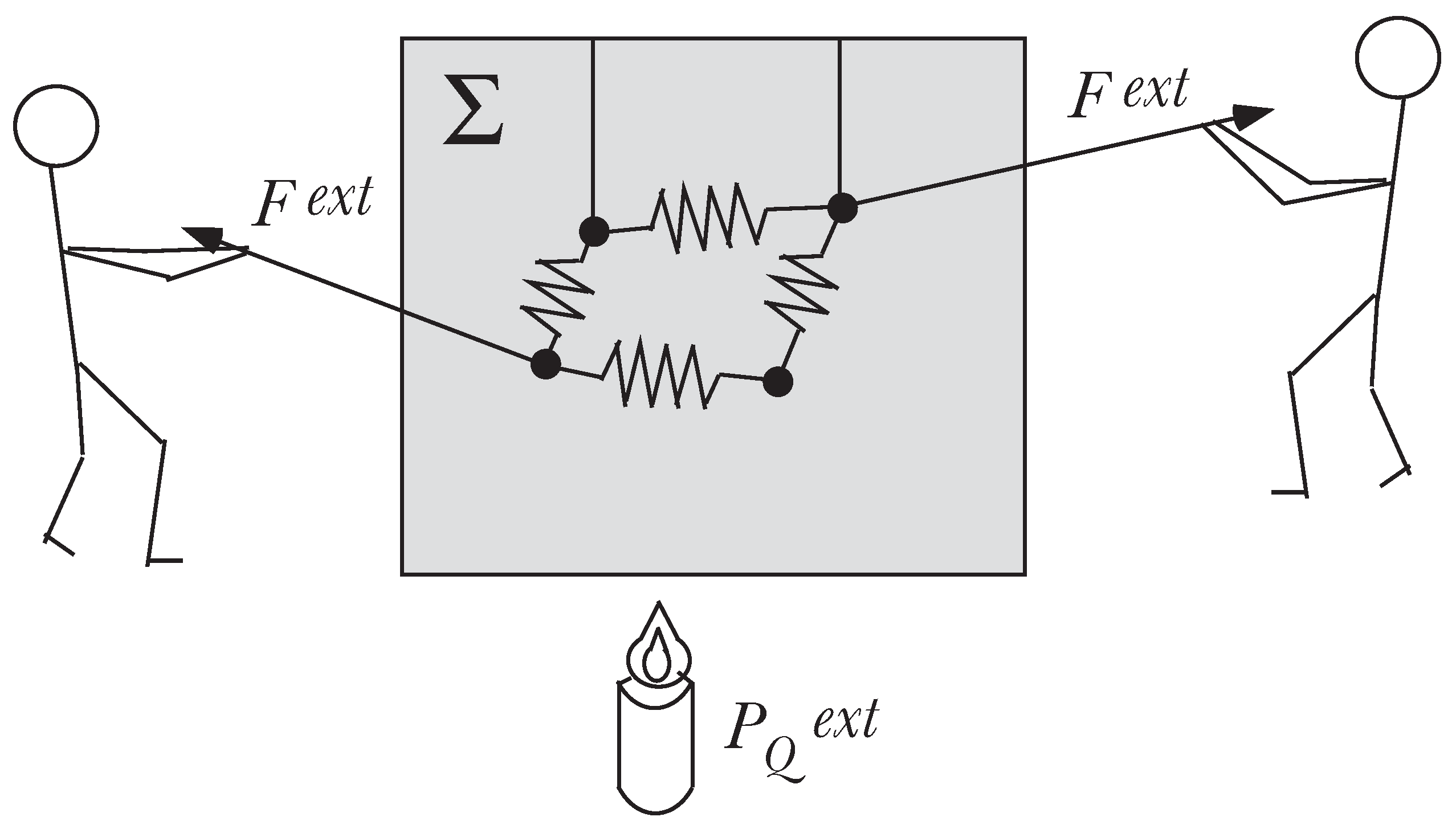
We consider a physical system Σ of N point particles imbedded in a fluid (e.g., air, water, ...) as shown in Figure 1. The point particles are submitted to holonomic, time-independent constraints, and we assume no a priori knowledge for the fluid.

The system is thus defined by the particles and the fluid. It is said to be isolated when there is no interaction between Σ and the outside (no external force, no heat exchange, no matter exchange). By definition, the mechanical state of Σ is defined by $2n$ independent variables $\xi =({\xi }^1,\dots ,{\xi }^{2n})=(q^1,\dots ,q^n,v^1,\dots ,v^n)$ where $q=(q^1,\dots ,q^n)$ are the generalised coordinates and $v=(v^1,\dots ,v^n)$, with $v^i=\frac{d{q}^i}{dt}$, are the generalised velocities. Moreover, under the above condition on the system, the kinetic energy K for N point particles of mass $m_{\alpha }$, defined as,

$$K=\frac{1}{2}\sum _{\alpha =1}^N{m}_{\alpha }{v}_{\alpha }^2,$$

(4)

is expressed in terms of the generalised coordinates $q_i$ and velocities $v_i$, by the quadratic form (see [6] Section 8.6)

$${\displaystyle K(q,v)=\frac{1}{2}\sum _{i,j=1}^n{g}_{ij}\left(q\right)v^i{v}^j⩾0,\mathrm{with}{g}_{ij}=g_{ji}.}$$

(5)

Furthermore, the exterior of the system can act on the generalised coordinate $q^i$ by means of a generalised force $Q_i^{\text{ext}}\left(t\right)$, and the work done per unit time by this force on Σ is the work-power ${P_W^{\text{ext}}}_i\left(t\right)=Q_i^{\text{ext}}\left(t\right)v^i$.

Figure 1. The system Σ: N particles imbedded in a fluid.

Figure 1. The system Σ: N particles imbedded in a fluid.

From observations, we conclude that the set of mechanical variables does not entirely define the state of the system and we are forced to introduce thermal variables. To simplify the following discussion, we assume that it is sufficient to add just one thermal variable to define entirely the state. Since in the axiomatic formulation of the second law there exists for any system a thermal observable, the entropy S, we shall define the state by the set of variables $\rho =\left(S,q,v\right)$, which are all independent by definition of the holonomic constraints.

For our system, we assume that the energy E, introduced in the first law, is the sum of the kinetic energy (5) and a potential energy U independent of the velocities, i.e.,

$$E(S,q,v)=K(q,v)+U(S,q).$$

(6)

The “potential energy” $U(S,q)$ describes the internal forces but may contain contributions from the outside of Σ, such as potentials of conservative external forces (e.g., the gravitational potential energy due to the earth). In this case, these forces are considered as internal forces of Σ, and not external.

Since the system is closed, i.e., there is no exchange of matter with the outside, the first law of thermodynamics reduces to,

$$\frac{dE}{dt}=P_W^{\text{ext}}\left(t\right)+P_Q^{\text{ext}}\left(t\right).$$

(7)

Using the fact that $E=E(S,q,v)$, the LHS side of the first law (7) gives,

$$\begin{array}{cc}\hfill \frac{dE}{dt}& =\frac{\partial E}{\partial S}\dot{S}+\sum _i\frac{\partial E}{\partial q^i}{\dot{q}}^i+\sum _i\frac{\partial E}{\partial v^i}{\dot{v}}^i\hfill \\ & =\frac{\partial U}{\partial S}\dot{S}+\frac{1}{2}\sum _{i,j,k}\frac{\partial g_{ij}}{\partial q^k}{v}^i{v}^j{v}^k+\sum _i\frac{\partial U}{\partial q^i}{v}^i+\sum _{i,j}{g}_{ij}{v}^i{\dot{v}}^j.\hfill \end{array}$$

(8)

At this point, we must insist on the fact that the choice of general coordinates was completely arbitrary. Therefore, we want to impose the covariance of the time evolution equations, i.e., they must have the same structure for any coordinate transformation of the mechanical variables,

$$\begin{array}{c}\hfill \begin{array}{cc}& q^{\prime i}=q^{\prime i}\left(q\right),\hfill \\ & v^{\prime i}=\sum _j\frac{\partial q^{\prime i}}{\partial q^j}{v}^j.\hfill \end{array}\end{array}$$

(9)

Under the covariance requirement, $g_{ij}$ must be a second order, symmetrical, covariant tensor so that K is a scalar. In order to ensure that K is positive definite, $g_{ij}$ must have a positive definite signature. Moreover, one can easily check that

$$\frac{dK}{dt}=\frac{1}{2}\sum _{i,j,k}\frac{\partial g_{ij}}{\partial q^k}{v}^i{v}^j{v}^k+\sum _{i,j}{g}_{ij}{v}^i{\dot{v}}^j,$$

(10)

is not covariant. However, the second term on the RHS of (8) is totally symmetric and invariant under cyclic permutation of indices, so that we have,

$$\frac{1}{2}\sum _{i,j,k}\frac{\partial g_{ij}}{\partial q^k}{v}^i{v}^j{v}^k=\sum _{i,j,k}\left(\frac{\partial g_{ij}}{\partial q^k}-\frac{1}{2}\frac{\partial g_{jk}}{\partial q^i}\right)v^i{v}^j{v}^k=\frac{1}{2}\sum _{i,j,k}\left(\frac{\partial g_{ij}}{\partial q^k}+\frac{\partial g_{ik}}{\partial q^j}-\frac{\partial g_{jk}}{\partial q^i}\right)v^i{v}^j{v}^k.$$

(11)

Introducing the symbols,

$${\Gamma }_{ijk}\left(q\right)=\frac{1}{2}\left(\frac{\partial g_{ij}}{\partial q^k}+\frac{\partial g_{ik}}{\partial q^j}-\frac{\partial g_{jk}}{\partial q^i}\right),$$

(12)

the LHS of the first law (7) reduces to the covariant equation,

$$\frac{dE}{dt}=\frac{\partial U}{\partial S}\dot{S}+\sum _i{v}^i\left(\sum _j{g}_{ij}{\dot{v}}^j+\sum _{j,k}{\Gamma }_{ijk}{v}^j{v}^k+\frac{\partial U}{\partial q_i}\right).$$

(13)

As for the RHS of (7), we have [6],

$$P_W^{\text{ext}}\left(t\right)=\sum _i{Q}_i^{\text{ext}}\left(t\right)v^i\left(t\right),$$

(14)

where $Q_i^{\text{ext}}\left(t\right)$ is the external generalised force associated with $q^i$.

It is useful to introduce two new state functions, defined respectively as,

$$\begin{array}{ccc}\hfill Q_i^{\text{int}}(S,q)& =& -\frac{\partial U}{\partial q^i},\hfill \end{array}$$

(15)

$$\begin{array}{ccc}\hfill T(S,q,v)& =& \frac{\partial U}{\partial S},\hfill \end{array}$$

(16)

where $Q_i^{\text{int}}(S,q)$ is the internal force associated with the generalised coordinate $q^i$ and $T(S,q,v)$ is called the “temperature” [3]. Using these definitions, the first law (7) reduces to the thermodynamic equation,

$$T\frac{dS}{dt}=\sum _i{v}^i\left(Q_i^{\text{ext}}\left(t\right)+Q_i^{\text{int}}-\sum _j{g}_{ij}{\dot{v}}^j-\sum _{j,k}{\Gamma }_{ijk}{v}^j{v}^k\right)+P_Q^{\text{ext}}\left(t\right).$$

(17)

4. System of Point Particles: Second Law

We investigate now the consequence of the second law for our system by proceeding in three steps: first, we consider an isolated system, then, we extend our analysis to an adiabatically closed system, finally, we generalise our approach to a closed system with heat exchange.

4.1. Thermodynamics of an Isolated System

An isolated system is characterised by the absence of interaction with the exterior, i.e., $Q_i^{\text{ext}}\left(t\right)=0$ and $P_Q^{\text{ext}}\left(t\right)=0$. In this case, it follows from (17) that

$$\dot{S}\left(t\right)=\frac{1}{T}\sum _i{v}^i\left(Q_i^{\text{int}}-\sum _j{g}_{ij}{\dot{v}}^j-\sum _{j,k}{\Gamma }_{ijk}{v}^j{v}^k\right).$$

(18)

This means that there exists a state function $I(S,q,v)$ called “entropy production” given by

$$I(S,q,v)=\frac{1}{T(S,q,v)}\sum _i{v}^i\left(Q_i^{\text{int}}-\sum _j{g}_{ij}{\dot{v}}^j-\sum _{j,k}{\Gamma }_{ijk}{v}^j{v}^k\right),$$

(19)

and such that

$$\dot{S}\left(t\right)=I(S\left(t\right),q\left(t\right),v\left(t\right)).$$

(20)

At this point, we introduce the state function $Q_i^{\text{fr}}(S,q,v)$, called “friction force associated with the generalised coordinate $q^i$”, defined as,

$$Q_i^{\text{fr}}=-Q_i^{\text{int}}+\sum _i{g}_{ij}{\dot{v}}^j+\sum _{j,k}{\Gamma }_{ijk}{v}^j{v}^k.$$

(21)

With this definition (21), the entropy production (19) can be expressed as,

$$I(S,q,v)=-\frac{1}{T}\sum _i{v}^i{Q}_i^{\text{fr}}.$$

(22)

This expression of the entropy production given as the products of the generalised velocities with the associated friction forces (or affinities) is analogous to the usual expression in nonequilibrium thermodynamics found for example in [7] (p. 309), [8] (p. 30) or [9] (p. 213). From the evolution part of the second law (2) (following the standard methods outlined in [3] p. 31, [8] p. 31, [9] pp. 215, 235, [10] p. 348) we must have, $I(S,q,v)⩾0$, and thus the friction force is of the form,

$$Q_i^{\text{fr}}(S,q,v)=-\sum _j{\lambda }_{ij}(S,q,v)v^j,$$

(23)

where the “friction coefficient tensor ${\lambda }_{ij}(S,q,v)$” must satisfy the non-negativity condition,

$$\frac{1}{T(S,q,v)}\left\{{\lambda }_{\left(ij\right)}(S,q,v)\right\}⩾0,\text{where}{\lambda }_{\left(ij\right)}=\frac{1}{2}\left({\lambda }_{ij}+{\lambda }_{ji}\right).$$

(24)

Note that in the usual linear scheme of non-equilibrium thermodynamics, i.e., near an equilibrium point, one considers ${\lambda }_{ij}$ to be the coefficients of a constant matrix computed at this equilibrium point, as explained in [9] (p. 236).

In conclusion, in this case, the entropy production is given by,

$$I(S,q,v)=\frac{1}{T(S,q,v)}\sum _{i,j}{\lambda }_{ij}(S,q,v)v^i{v}^j⩾0.$$

(25)

Thus, we have obtained the time evolution equations for the isolated system,

$$\left\{\begin{array}{cc}{\displaystyle \sum _j{g}_{ij}{\ddot{q}}^j+\sum _{j,k}{\Gamma }_{ijk}{\dot{q}}^j{\dot{q}}^k=-\frac{\partial U}{\partial q^i}-\sum _j{\lambda }_{ij}{\dot{q}}^j}\hfill & \text{mechanical}\text{equations}\hfill \\ {\displaystyle \frac{dS}{dt}=\frac{1}{T}\sum _{i,j}{\lambda }_{ij}{\dot{q}}^i{\dot{q}}^j}\hfill & \text{thermal}\text{equation}\hfill \end{array}\right.$$

(26)

Hence, in such a phenomenological approach, the system is characterised by the state functions $g_{ij}\left(q\right)$, $U(S,q)$ and ${\lambda }_{ij}(S,q,\dot{q})$, which have to be determined experimentally. It should be stressed that $Q_i^{\text{int}}=-\frac{\partial U}{\partial q^i}$ is an internal conservative force (e.g., the force exerted between two particles) introduced in the first law and that $Q_i^{\text{fr}}$ is a friction force exerted by the fluid in which the particles are imbedded. Note that in the particular case of solid friction, the friction force is singular [2].

4.2. Thermodynamics of an Adiabatically Closed System

We now consider an adiabatically closed system, i.e., $P_Q^{\text{ext}}\left(t\right)=0$, for which the thermodynamic equation (17) reduces to,

$$T\frac{dS}{dt}=\sum _i{v}^i\left(Q_i^{\text{ext}}\left(t\right)+Q_i^{\text{int}}-\sum _j{g}_{ij}{\dot{v}}^j-\sum _{j,k}{\Gamma }_{ijk}{v}^j{v}^k\right).$$

(27)

Again, we introduce the generalised friction force,

$$Q_i^{\text{fr}}=-Q_i^{\text{ext}}\left(t\right)-Q_i^{\text{int}}+\sum _j{g}_{ij}{\dot{v}}^j+\sum _{j,k}{\Gamma }_{ijk}{v}^j{v}^k,$$

(28)

which yields,

$$T\frac{dS}{dt}=-\sum _i{v}^i{Q}_i^{\text{fr}},$$

(29)

and

$$\sum _j{g}_{ij}{\dot{v}}^j+\sum _{j,k}{\Gamma }_{ijk}{v}^j{v}^k=Q_i^{\text{int}}+Q_i^{\text{fr}}+Q_i^{\text{ext}}\left(t\right).$$

(30)

Since the system is adiabatically closed, the evolution part of the second law (2) implies again,

$$\frac{dS}{dt}=I\left(t\right)=-\frac{1}{T}\sum _i{v}^i{Q}_i^{\text{fr}}⩾0,$$

(31)

which suggests that the friction force has the same form as for the isolated system,

$$Q_i^{\text{fr}}=-\sum _j{\lambda }_{ij}(S,q,v)v^j,$$

(32)

and thus is again a state function with the same coefficients ${\lambda }_{ij}$ as in the isolated case. Similarly to the isolated system, the time evolution equations are given by,

$$\left\{\begin{array}{cc}{\displaystyle \sum _j{g}_{ij}{\ddot{q}}^j+\sum _{j,k}{\Gamma }_{ijk}{\dot{q}}^j{\dot{q}}^k=-\frac{\partial U}{\partial q^i}-\sum _j{\lambda }_{ij}{\dot{q}}^j+Q_i^{\text{ext}}\left(t\right)}\hfill & \text{mechanical}\text{equations}\hfill \\ {\displaystyle \frac{dS}{dt}=\frac{1}{T}\sum _{i,j}{\lambda }_{ij}{\dot{q}}^i{\dot{q}}^j}\hfill & \text{thermal}\text{equation}\hfill \end{array}\right.$$

(33)

It is worth mentioning that the arbitrary external force $Q_i^{\text{ext}}\left(t\right)$ should not be confused with the internal forces, which are the conservative force $Q_i^{\text{int}}$ and the dissipative friction force $Q_i^{\text{fr}}$.

4.3. Thermodynamics of a Closed System

We now consider a closed system, i.e., $P_{\text{chem}}^{\text{ext}}\left(t\right)=0$, for which the thermodynamic equation is given by (17). The entropy variation of the system is due to the friction force (28), as for the isolated and adiabatically closed systems, but also to heat exchange with the exterior according to (17) i.e.,

$$T\frac{dS}{dt}=-\sum _i{v}^i{Q}_i^{\text{fr}}+P_Q^{\text{ext}}\left(t\right).$$

(34)

Hence, similarly to the isolated and adiabatically closed systems, the time evolution equations are given by,

$$\left\{\begin{array}{cc}{\displaystyle \sum _j{g}_{ij}{\ddot{q}}^j+\sum _{j,k}{\Gamma }_{ijk}{\dot{q}}^j{\dot{q}}^k=-\frac{\partial U}{\partial q^i}-\sum _j{\lambda }_{ij}{\dot{q}}^j+Q_i^{\text{ext}}\left(t\right)}\hfill & \text{mechanical}\text{equations}\hfill \\ {\displaystyle \frac{dS}{dt}=\frac{1}{T}\sum _{i,j}{\lambda }_{ij}{\dot{q}}^i{\dot{q}}^j+\frac{1}{T}{P}_Q^{\text{ext}}\left(t\right)}\hfill & \text{thermal}\text{equation}\hfill \end{array}\right.$$

(35)

4.4. Equilibrium Part of the Second Law

Finally, we can investigate the consequences of the equilibrium part of the second law (3). In this case, we have to assume that the system is isolated for all $t⩾t_0$ and we have to look for the maximum of S under the condition that the energy $E(S,q,v)=\overline{E}$ is fixed. In other words, we have to look for the maximum of $S(\overline{E},q,v)$.

One can show [3] that this maximum condition on S is equivalent to the condition that the energy $E(S,q,v)$ is minimum for a fixed $S=\overline{S}$ if the temperature T is positive, and is maximum if T is negative, i.e.,

$${\delta }^{\left(1\right)}E{|}_{S=\overline{S}}=0,\text{and}\frac{1}{T}{\delta }^{\left(2\right)}E{|}_{S=\overline{S}}⩾0.$$

(36)

(i)

The extremum condition ${\delta }^{\left(1\right)}E{|}_{S=\overline{S}}=0$ implies that,

• ${\displaystyle \frac{\partial E}{\partial v^i}{|}_{S=\overline{S}}=0\text{i.e.,}\sum _j{g}_{ij}\left(q\right)v^j=0\text{and}\text{thus}{v}^j=0\text{since}{g}_{ij}\text{is}\text{positive}\text{definite.}}$
• ${\displaystyle \frac{\partial E}{\partial q^i}{|}_{S=\overline{S}}=0\text{which}\text{gives}\text{(with}{v}^j=0\text{)},Q^{\text{int}}=-\frac{\partial U}{\partial q^i}=0.}$
  In other words, the extremum condition implies that the system evolves to an equilibrium point of the time evolution equation (26), characterised by $q=\overline{q}$ and $v=\overline{v}=0$.

(ii)

The condition $\frac{1}{T}{\delta }^{\left(2\right)}E{|}_{S=\overline{S},q=\overline{q},v=\overline{v}=0}⩾0$ implies first that the matrix $\frac{1}{T}{g}_{ij}\left(\overline{q}\right)$ is non-negative and thus, for our mechanical system with positive kinetic energy, the temperature is necessarily positive. This in turn implies that the friction coefficients matrix is non-negative. Moreover, this same condition also implies that the matrix $\frac{1}{T}\frac{{\partial }^{2}U}{\partial q^i\partial q^j}\left(\overline{S},\overline{q}\right)$ must be non-negative. In conclusion, the equilibrium part of the second law implies that the system evolves towards a stable equilibrium point. This is the zeroth law of thermodynamics [3].

5. From Thermodynamics to Mechanics

The symmetric matrix $g_{ij}$ can be identified as a metric with a positive definite signature on the configuration space. Thus, the configuration space is a Riemannian manifold endowed with a torsion-free Levi-Civita connection [11], where the components,

$${\Gamma }_{ijk}\left(q\right)=\frac{1}{2}\left(\frac{\partial g_{ij}}{\partial q^k}+\frac{\partial g_{ik}}{\partial q^j}-\frac{\partial g_{jk}}{\partial q^i}\right),$$

(37)

are commonly referred to as the Riemann-Christoffel symbols. Such a manifold preserves the generalised infinitesimal distances squared $d{s}^2$ defined in terms of the generalised coordinates as [12],

$$d{s}^2=\sum _{i,j}{g}_{ij}\left(q\right)d{q}^{i}d{q}^j,$$

(38)

and satisfies the metricity condition [13], which requires the covariant derivative of the metric with respect to every coordinate $q^i$ to vanish,

$${\nabla }_i{g}_{jk}=0.$$

(39)

In the particular case of an isolated system where the friction coefficients matrix is strictly zero, then from the second relation in (26), the entropy is necessarily constant. Furthermore, if the potential energy is zero, i.e., $U=0$, then the evolution of the system is a geodesic in configuration space given by,

$${\dot{v}}^i+\sum _{j,k}{{\Gamma }^i}_{jk}{v}^j{v}^k=0,$$

(40)

thus satisfying the 1st law of Newton.

At this point, it is convenient to introduce the Lagrangian of the system defined as,

$$\mathcal{L}(S,q,\dot{q})=K(q,\dot{q})-U(S,q)=\frac{1}{2}\sum _{i,j}{g}_{ij}{\dot{q}}^i{\dot{q}}^j-U(S,q).$$

(41)

In order to recast the dynamical terms on the RHS of the thermodynamic equation (17) in an analytical manner, we compute the partial derivatives of the Lagrangian and their time derivatives,

$$\begin{array}{cc}& {\displaystyle {\displaystyle \frac{\partial \mathcal{L}}{\partial q^i}}={\displaystyle \frac{1}{2}}\sum _{j,k}{\displaystyle \frac{\partial g_{jk}}{\partial q^i}}{\dot{q}}^j{\dot{q}}^k-{\displaystyle \frac{\partial U}{\partial q^i}},}\hfill \end{array}$$

(42)

$$\begin{array}{cc}& {\displaystyle {\displaystyle \frac{d}{dt}}\left({\displaystyle \frac{\partial \mathcal{L}}{\partial {\dot{q}}^i}}\right)=\sum _j{g}_{ij}{\ddot{q}}^j+\sum _{j,k}{\displaystyle \frac{\partial g_{ij}}{\partial q^k}}{\dot{q}}^j{\dot{q}}^k=\sum _j{g}_{ij}{\ddot{q}}^j+{\displaystyle \frac{1}{2}}\sum _{j,k}\left({\displaystyle \frac{\partial g_{ij}}{\partial q^k}}+{\displaystyle \frac{\partial g_{ik}}{\partial q^j}}\right){\dot{q}}^j{\dot{q}}^k.}\hfill \end{array}$$

(43)

From the differential relations (42) and (43), we derive the dynamic identity,

$$\frac{d}{dt}\left({\displaystyle \frac{\partial \mathcal{L}}{\partial {\dot{q}}^i}}\right)-\frac{\partial \mathcal{L}}{\partial q^i}=\sum _j{g}_{ij}{\ddot{q}}^j+\sum _{j,k}{\Gamma }_{ijk}{\dot{q}}^j{\dot{q}}^k+\frac{\partial U}{\partial q^i}.$$

(44)

Using this identity, the thermodynamic equation (35) reduces to,

$$\left\{\begin{array}{cc}{\displaystyle {\displaystyle \frac{d}{dt}}\left({\displaystyle \frac{\partial \mathcal{L}}{\partial {\dot{q}}^i}}\right)-{\displaystyle \frac{\partial \mathcal{L}}{\partial q^i}}=Q_i^{\text{ext}}\left(t\right)-\sum _j{\lambda }_{ij}{\dot{q}}^j}\hfill & \text{Lagrange}\text{equations}\hfill \\ {\displaystyle \frac{dS}{dt}=\frac{1}{T}\sum _{i,j}{\lambda }_{ij}{\dot{q}}^i{\dot{q}}^j+\frac{1}{T}{P}_Q^{\text{ext}}\left(t\right)}\hfill & \text{Thermal}\text{equation}\hfill \end{array}\right.$$

(45)

In conclusion, if the state functions U and ${\lambda }_{ij}$ are independent of S, or equivalently, if the time evolution happens at fixed temperature by contact with a thermal bath, the mechanical Lagrange equations decouple from the thermal equation. This is the usual case considered in mechanics.

6. Thermodynamics of an Isolated System of Point Particles Interacting through a Harmonic Potential

As an application of the formalism we developed, we now consider the thermodynamics of an isolated system where the state functions U and ${\lambda }_{ij}$ are independent of S. The system consists of identical point particles interacting through a harmonic potential and is the simplest phenomenological model of a solid, where the harmonic oscillators represent the phonons. As generalised coordinates, we choose for simplicity cartesian coordinates of the point particles and denote them $q=x$. Thus, the metric reduces to the trivial Kronecker delta, i.e., $g_{ij}\left(q\right)={\delta }_{ij}$. The kinetic energy $K(x,\dot{x})$ of the point particles per unit mass and the harmonic interaction potential per unit mass $U\left(x\right)$ are respectively given by,

$$\begin{array}{cc}& {\displaystyle K(x,\dot{x})={\displaystyle \frac{1}{2}}\sum _{i,j}{\delta }_{ij}{\dot{x}}^i{\dot{x}}^j,}\hfill \end{array}$$

(46)

$$\begin{array}{cc}& {\displaystyle U\left(x\right)={\displaystyle \frac{1}{2}}{\omega }^2\sum _{i,j,k,l}{\delta }_{ij}{\delta }_{kl}\left(x^i-x^k\right)\left(x^j-x^l\right),}\hfill \end{array}$$

(47)

where the coefficient ${\omega }^2$ is positive by the equilibrium condition of the second law and ω represents the angular frequency of the identical harmonic oscillators. The Lagrangian of the system is given by,

$${\displaystyle \mathcal{L}(x,\dot{x})={\displaystyle \frac{1}{2}}\sum _{i,j}{\delta }_{ij}{\dot{x}}^i{\dot{x}}^j-{\displaystyle \frac{1}{2}}{\omega }^2\sum _{i,j,k,l}{\delta }_{ij}{\delta }_{kl}\left(x^i-x^k\right)\left(x^j-x^l\right).}$$

(48)

The partial derivatives of the Lagrangian and their time derivatives are given by,

$$\begin{array}{cc}& {\displaystyle \frac{\partial \mathcal{L}}{\partial x^i}}=-{\omega }^2\sum _{j,k,l}{\delta }_{ij}{\delta }_{kl}\left(x^j-x^l\right),\hfill \end{array}$$

(49)

$$\begin{array}{cc}& {\displaystyle {\displaystyle \frac{d}{dt}}\left({\displaystyle \frac{\partial \mathcal{L}}{\partial {\dot{x}}^i}}\right)={\displaystyle \frac{d}{dt}}\left({\displaystyle \sum _j{\delta }_{ij}{\dot{x}}^j}\right)=\sum _j{\delta }_{ij}{\ddot{x}}^j.}\hfill \end{array}$$

(50)

Finally, the system of coupled thermodynamical equations (26) is explicitly found to be,

$$\left\{\begin{array}{cc}{\displaystyle \sum _j\left[{\displaystyle {\delta }_{ij}{\ddot{x}}^j+{\lambda }_{ij}{\dot{x}}^j+{\omega }^2{\delta }_{ij}\sum _{k,l}{\delta }_{kl}\left(x^j-x^l\right)}\right]=0}\hfill & \text{Lagrange}\text{equations}\hfill \\ {\displaystyle \frac{dS}{dt}=\frac{1}{T}\sum _{i,j}{\lambda }_{ij}{\dot{x}}^i{\dot{x}}^j}\hfill & \text{Thermal}\text{equation}\hfill \end{array}\right.$$

(51)

The physical interpretation of these evolution equations is clear [6]. The Lagrange equations are a system of coupled damped harmonic oscillators where the damping term is due to the action of a viscous friction force. These equations are in turn coupled to the thermal equation through the friction force. Since ${\lambda }_{ij}$ and ${\omega }^2$ do not depend on S, the Lagrange equations can be solved independently to find $x\left(t\right)$, which in turn will give $S\left(t\right)$ using the thermal equation.

If the friction matrix $\left\{{\lambda }_{ij}\right\}$ is positive, the condition that the system evolves to a state of maximal entropy implies that the system evolves towards the equilibrium state (${\overline{x}}^i=0$, ${\dot{\overline{x}}}^i=0$). For a strictly mechanical system, i.e., if ${\lambda }_{ij}=0$, then S is a constant; in this case the system will oscillate around the equilibrium state according to,

$$\left\{\begin{array}{cc}{\displaystyle {\ddot{x}}^i+{\omega }^2\sum _j\left(x^i-x^j\right)=0}\hfill & \text{Lagrange}\text{equations}\hfill \\ {\displaystyle S=\text{const}}\hfill & \text{Thermal}\text{equation}\hfill \end{array}\right.$$

(52)

7. Conclusions

We followed the phenomenological approach developed by Stückelberg to study a closed thermodynamic system consisting of a fixed number of point particles. We thus obtained a system of coupled differential equations describing the thermodynamic evolution of the system. We observed that in this system of differential equations, the coupling between the Lagrange equations and the thermal equation is due to the viscous friction terms. If the phenomenological variables U, ${\lambda }_{ij}$, do not depend on S, we recover the usual Newton or Lagrange equations with friction. In the general case where these variables do depend on S, i.e., on temperature, such a coupling shows that thermodynamics is a natural extension of mechanics. Finally, we applied our coupled thermodynamic equations to study the thermodynamics of an isolated system consisting of identical point particles interacting through a harmonic potential, which is the simplest phenomenological model of a solid.

References

1. Carnot, S. Réflexions sur la puissance motrice du feu et sur les machines propres à développer cette puissance; Bachelier: Paris, France, 1824. [Google Scholar]
2. Ferrari, C.; Gruber, C. Friction force: from mechanics to thermodynamics. Eur. J. Phys. 2010, 31, 1159–1175. [Google Scholar] [CrossRef]
3. Stückelberg von Breidenbach, E.C.G.; Scheurer, P.B. Thermociétique Phénoménologique Galiléenne; Birkhauser: Basel, Switzerland, 1974. [Google Scholar]
4. Fuchs, H.U. The Dynamics of Heat; Springer: New York, NY, USA, 1996. [Google Scholar]
5. Gruber, C. Thermodynamics of systems with internal adiabatic constraints: time evolution of the adiabatic piston. Eur. J. Phys. 1999, 20, 259–266. [Google Scholar] [CrossRef]
6. Goldstein, H.; Poole, C.; Safko, J.; Addison, S.R. Classical Mechanics, 3rd ed.; Addison Wesley: White Plains, NY, USA, 2002; Volume 70, pp. 782–783. [Google Scholar]
7. Callen, H.B. Thermodynamics and an Introduction to Thermostatistics, 2nd ed.; John Wiley and Sons, Inc.: New York, NY, USA, 1985. [Google Scholar]
8. de Groot, S.R.; Mazur, P. Non-equilibrium thermodynamics; Dover: New York, NY, USA, 1984. [Google Scholar]
9. Prigogine, I.; Kondepudi, D. Thermodynamique; Odile Jacob: Paris, France, 1999. [Google Scholar]
10. Perez, J.P. Thermodynamique; Masson: Paris, France, 1997. [Google Scholar]
11. Weinberg, S. Gravitation and Cosmology: Principles and Applications of the General Theory of Relativity; John Wiley and Sons: New York, NY, USA, 1972. [Google Scholar]
12. Hobson, M.P.; Efstathiou, G.P.; Lasenby, A.N. General Relativity; Cambridge University Press: Cambridge, UK, 2006. [Google Scholar]
13. Brechet, S.D.; Hobson, M.P.; Lasenby, A.N. Classical big-bounce cosmology: dynamical analysis of a homogeneous and irrotational Weyssenhoff fluid. Classical Quant. Grav. 2008, 25, 245016. [Google Scholar] [CrossRef]