Microcanonical Description of (Micro) Black Holes

Abstract

The microcanonical ensemble is the proper ensemble to describe black holes which are not in thermodynamic equilibrium, such as radiating black holes. This choice of ensemble eliminates the problems, e.g., negative specific heat (not allowed in the canonical ensemble) and loss of unitarity, encountered when the canonical ensemble is used. In this review we present an overview of the weaknesses of the standard thermodynamic description of black holes and show how the microcanonical approach can provide a consistent description of black holes and their Hawking radiation at all energy scales. Our approach is based on viewing the horizon area as yielding the ensemble density at fixed system energy. We then compare the decay rates of black holes in the two different pictures. Our description is particularly relevant for the analysis of micro-black holes whose existence is predicted in models with extra-spatial dimensions.

1. Introduction

Entropy as originally defined by Clausius is a statement about the change of energy with respect to temperature for systems in thermodynamic equilibrium. Later a correlation between entropy and the statistical mechanical probability of finding a system in a given state was obtained. The latter can be generalized to include systems which are not in thermodynamic equilibrium and for which the microcanonical ensemble is the proper ensemble to describe the system. Since the microcanonical ensemble requires conservation of energy for any system to which it is applied, it is the proper ensemble to describe microscopic black holes. However, in spite of its many mathematical and physical inconsistencies and drawbacks, the treatment of black holes as thermodynamical systems has since its inception been the description preferred by most physicists investigating the nature of black holes. Not least among the drawbacks is the fact that the laws of quantum mechanics are violated, because the number density function of the emitted radiation as calculated using a thermal vacuum is characteristic of mixed states, while the incoming radiation may have been in pure states. Since black holes can in principle radiate away completely, the unitarity principle is violated.

In a series of papers [1,2,3,4,5,6,7,8,9] we have investigated an alternative description of black holes which is free of the encountered problems in the thermodynamical approach. In this review, we shall first recall the main aspects of our approach and then proceed to describe its application to microscopic black holes [10,11,12,13,14,15,16,17,18,19,20,21,22,23]. The latter are predicted to exist in models with extra spatial dimensions [24,25,26,27], and an extensive analysis of their possible phenomenological appearance can be found in [10,11,28,29,30,31,32,33,34,35,36,37,38,39,40,41,42,43,44,45].

In Section 2 we present a brief summary of the thermodynamical description of processes involving black holes and discuss in detail the inconsistencies mentioned above; in Section 3 we briefly review Schwarzschild black holes in more than four dimensions; In Section 4 we discuss the thermodynamical interpretation of black holes within the context of mean field theory and show that the thermal vacuum is the false vacuum for a black hole system. We also present an alternative vacuum for such a system and the microcanonical number density which corresponds to this vacuum. In Section 5 we present the microcanonical wave functions for the in and out states and in Section 6 we derive the black hole decay rates for micro-black holes in models with extra dimensions.

We shall either use natural units $c={\ell }_{\mathrm{p}}=M_{\mathrm{p}}=1$ or show explicitly ${\ell }_{\mathrm{p}}$ and $M_{\mathrm{p}}$ or the equivalent scales ${\ell }_{\left(D\right)}$ and $M_{\left(D\right)}$ in models with extra spatial dimensions. We shall also use the scale $M_{\mathrm{ew}}\simeq 1$TeV.

2. Thermodynamical Interpretation of Black Holes

Bekenstein’s original observation [46,47] that the area of a black hole (in units of the Planck area ${\ell }_{\mathrm{p}}^2$) is analogous to the thermodynamical entropy,

$$\begin{array}{c}\hfill S_{\mathrm{H}}=\frac{A}{4}\end{array}$$

(1)

was enlarged upon in [48] where the four laws of black hole thermodynamics were hypothesized. The mass difference of neighboring equilibrium states was shown to be related to the change in the black hole area A by the Smarr formula,

$$\begin{array}{c}\hfill \Delta M=\kappa \Delta A+\varpi \Delta J+\Phi \Delta Q\end{array}$$

(2)

where κ is the surface gravity related to the temperature by

$$\begin{array}{c}\hfill T={\beta }_{\mathrm{H}}^{-1}=\frac{\kappa }{2\pi }\end{array}$$

(3)

J is the angular momentum of the black hole, Q its charge and ϖ, Φ play the role of potentials. The partition function for the black hole is assumed to be

$$\begin{array}{c}\hfill Z\left(\beta \right)=\mathrm{Tr}{e}^{-\beta H}=e^{-S_{\mathrm{H}}}\end{array}$$

(4)

where $S_{\mathrm{H}}$ is the Hawking entropy,

$$\begin{array}{c}\hfill S_{\mathrm{H}}=S_E-{\beta }_{\mathrm{H}}\varpi J\end{array}$$

(5)

and $S_E$ the Euclidean action. Finally, in thermodynamical equilibrium the statistical mechanical density of states is given by

$$\begin{array}{c}\hfill \Omega =Z^{-1}\left(\beta \right)=e^{S_{\mathrm{H}}}\end{array}$$

(6)

and the specific heat

$$\begin{array}{c}\hfill C_V=\frac{\partial E}{\partial T}=-\frac{{\beta }^2}{8\pi }<0\end{array}$$

(7)

which is a clear signal that the thermodynamical analogy fails.

A second problem can be best shown if we specialize the previous expressions to the Schwarzschild black hole, for which $S_{\mathrm{H}}=S_E=4\pi M^2$ and

$$\begin{array}{c}\hfill {\beta }_{\mathrm{H}}=8\pi M\end{array}$$

(8)

It then follows that the partition function as calculated from the microcanonical density of states,

$$\begin{array}{c}\hfill Z\left(\beta \right)={\int }_0^{\infty }dM\Omega \left(M\right)e^{-\beta M}={\int }_0^{\infty }dM{e}^{4\pi M^2}{e}^{-\beta M}\to \infty \end{array}$$

(9)

is infinite for all temperatures and hence the canonical ensemble is not equivalent to the (more fundamental) microcanonical ensemble, as is required for thermodynamical equilibrium.

The inequivalence of the two ensembles in systems with long-range interactions, such as gravity, has been investigated extensively (see, for example, the review [49] for a presentation of this issue in the astrophysical context). However, statistical mechanical theorems show that the specific heat can be negative in the microcanonical ensemble (where energy is held fixed) but must be necessarily positive in the canonical ensemble (where temperature is fixed). The above result (7) therefore should be more properly interpreted as implying that the microcanonical ensemble can be used for a black hole, whereas the canonical ensemble is not well-defined and should only be viewed as a useful approximation as long as the temperature does not change significantly on the time scale of interest.

In fact, if quantum mechanical effects are taken into account, black holes can be shown to evaporate and, according to the canonical picture, the emitted radiation has a Planckian distribution [50,51],

$$\begin{array}{c}\hfill n_{{\beta }_{\mathrm{H}}}\left(\omega \right)=\frac{1}{e^{{\beta }_{\mathrm{H}}\omega }-1}\end{array}$$

(10)

This implies that the black hole mass M will decrease in time, whereas the temperature ${\beta }_{\mathrm{H}}^{-1}\sim M^{-1}$ will increase (possibly) without bounds. Moreover, since in the standard Hawking’s picture black holes can in principle radiate away completely, this result implies that information can be lost, because pure states can come into the black hole but only mixed states come out. The breakdown of the unitarity principle is one of the most serious drawbacks of the thermodynamical interpretation, since it would require the replacement of quantum mechanics with some new (unspecified) physics. In order to avoid this scenario, some approaches predict the evaporation leaves a “black hole remnant” [52,53], as follows from assuming generalized uncertainty principles [54] and within models of non-commutative geometry [55].

3. Black Holes in D Dimensions

The inconsistencies of the thermodynamical interpretation are an indication that the interpretation of Equation (4) as the canonical partition function is wrong. In analogy with the usual WKB approximation, we instead hypothesize that

$$\begin{array}{c}\hfill P\simeq e^{-S_{\mathrm{H}}}\end{array}$$

(11)

is the probability for the transition from the metastable vacuum, namely the black hole semiclassical vacuum, to the true vacuum state with no black hole. This interpretation holds for any kind of black hole. The picture of particles tunneling through the horizon is technically not accurate, because the horizon is a causal boundary, not a potential barrier. Such a potential might be generated if the backreactions of the emitted particles are taken into account [56,57]. However, the distribution of emitted particles is decidedly non-thermal for such a potential. The quantum degeneracy of states for the system is proportional to $P^{-1}$ and is then given by

$$\begin{array}{c}\hfill \sigma \simeq c{e}^{A/4}\end{array}$$

(12)

where the constant c is determined from quantum field theoretic corrections and can contain non-local effects.

Explicit expressions can be obtained for the above quantities for some geometries. We shall here just consider the D-dimensional Schwarzschild black hole [58],

$$\begin{array}{c}\hfill d{s}^2=-e^{2\lambda }d{\tau }^2+e^{-2\lambda }d{r}^2+r^{2}d{\Omega }_{D-2}^2\end{array}$$

(13)

where

$$\begin{array}{c}\hfill e^{2\lambda }=1-{\left(\frac{r_{\mathrm{H}}}{r}\right)}^{D-3}\end{array}$$

(14)

The horizon area in D dimensions is

$$\begin{array}{c}\hfill \frac{A}{4}=\frac{A_{D-2}}{16\pi }{\beta }_{\mathrm{H}}{r}_{\mathrm{H}}^{D-2}\end{array}$$

(15)

with

$$\begin{array}{c}\hfill M=\frac{D-2}{16\pi }{A}_{D-2}{r}_{\mathrm{H}}^{D-3}\end{array}$$

(16)

where $A_{D-2}$ is the area of a unit $(D-2)$-sphere. Eliminating the horizon radius $r_{\mathrm{H}}$ in favor of the mass, the area becomes

$$\begin{array}{c}\hfill \frac{A}{4}=C\left(D\right)M^{\frac{D-2}{D-3}}\end{array}$$

(17)

where $C\left(D\right)$ is the mass-independent function

$$\begin{array}{c}\hfill C\left(D\right)=\frac{4^{\frac{D-1}{D-3}}{\pi }^{\frac{D-2}{D-3}}}{(D-3){(D-2)}^{\frac{D-2}{D-3}}{A}_{D-2}^{\frac{1}{D-3}}}\end{array}$$

(18)

From the above, we obtain the degeneracy of states

$$\begin{array}{c}\hfill \sigma \left(M\right)\simeq {\Omega }^{-1}\left(M\right)\simeq cexp\left[C\left(D\right)M^{\frac{D-2}{D-3}}\right]\end{array}$$

(19)

Comparing this expression to those known for non-local field theories, we find that it corresponds to the degeneracy of states for an extended quantum object (p-brane) of dimension $p=\frac{D-2}{D-4}$. As has been demonstrated by several authors [59,60,61], an exponentially rising density of states is the clear signal of a non-local field theory. P-brane theories are the only known non-local theories in theoretical physics which can give rise to exponentially rising degeneracies.

It is important to remark here that all dimensional quantities are evaluated in units of the corresponding Planck scale. For example, M in Equation (19) is actually $M/M_{\mathrm{P}}$ in $D=4$ dimensions. In models with extra spatial dimensions, $M_{\mathrm{P}}\sim {10}^{16}$TeV is replaced by a fundamental gravitational mass $M_{\left(D\right)}$ which could be as low as $M_{\mathrm{ew}}\simeq 1$TeV. In the following, we shall consider two such scenarios: the ADD case [24,25,26] with compact extra dimensions, and the RS case [27] with one possibly very large extra dimension.

4. Quantum Field Theory on Black Hole Backgrounds

To study particle production and propagation in black hole geometries we now turn to the mean field approximation in which fields are quantized on a classical black hole background. Since black holes have non-trivial topologies which causally separate two regions of space, the number of degrees of freedom is doubled, and two Fock spaces are required to describe quantum processes occurring in the vicinity of a black hole. Calculations of quantities associated with such processes can be carried out in ways analogous to calculations in Thermofield Dynamics [62], but with an overall fixed energy [9].

4.1. Canonical Formulation

The thermal vacuum for quantum fields scattered off of black holes can be written as

$$\begin{array}{c}\hfill |\mathrm{out};0\rangle =\frac{1}{Z^{1/2}\left({\beta }_{\mathrm{H}}\right)}\sum _{n=0}^{\infty }{e}^{-{\beta }_{\mathrm{H}}n\omega /2}|n\rangle \otimes |\tilde{n}\rangle \end{array}$$

(20)

with the partition function

$$\begin{array}{c}\hfill Z\left(\beta \right)=\sum _{n=0}^{\infty }{e}^{-\beta n\omega }\end{array}$$

(21)

and the states $|\tilde{n}\rangle$ are a complete orthonormal basis for the region of space causally disconnected from an external observer. Operators corresponding to physically measurable quantities are defined on the basis set $|n\rangle$ for states outside the horizon. The ensemble average (expectation value) of a physical observable $\widehat{O}$ in the $out$ region is

$$\begin{array}{c}\hfill \langle \mathrm{out};0|\widehat{O}|\mathrm{out};0\rangle =\frac{1}{Z\left({\beta }_{\mathrm{H}}\right)}\sum _n{e}^{-n{\beta }_{\mathrm{H}}\omega }\langle n|\widehat{O}|n\rangle \end{array}$$

(22)

where the temperature is given in Equation (3). For example, if $\widehat{O}$ is the number operator for particles of rest mass m, the ensemble average given in Equation (22) is the particle number density (10).

To describe particle interactions one then needs the (thermal) particle propagator,

$$\begin{array}{c}\hfill {\Delta }_{{\beta }_{\mathrm{H}}}=\frac{1}{k^2-m^2+iϵ}-2\pi i\delta (k^2-m^2)n_{{\beta }_{\mathrm{H}}}(m,k)\end{array}$$

(23)

with $n_{{\beta }_{\mathrm{H}}}$ given by Equation (10). These expressions are valid if black holes are described by a local field theory. However, as discussed in Section 2, the particle number distribution given in Equation (10) implies loss of coherence. The $in$ state is a pure state

$$\begin{array}{c}\hfill |\mathrm{in};0\rangle =|0\rangle \otimes |\tilde{0}\rangle \end{array}$$

(24)

but the number density obtained from the outgoing states is a thermal distribution.

In the microcanonical approach non-local effects can be taken into account by summing over all possible masses (angular momenta and charges)

$$\begin{array}{c}\hfill n_{{\beta }_{\mathrm{H}}}\left(k\right)={\int }_0^{\infty }dm\sigma \left(m\right)n_{{\beta }_{\mathrm{H}}}(m,k)\end{array}$$

(25)

Inclusion of non-local effects changes the thermal vacuum to

$$\begin{array}{c}\hfill |\mathrm{out};0\rangle =\frac{1}{Z^{1/2}\left({\beta }_{\mathrm{H}}\right)}\left[\prod _{m,k}\sum _{n_{k,m}=0}^{\infty }\right]\prod _{m,k}{e}^{-{\beta }_{\mathrm{H}}{n}_{k,m}{\omega }_{k,m}/2}|n_{k,m}\rangle \otimes |{\tilde{n}}_{k,m}\rangle \end{array}$$

(26)

where the quantity in square brackets represents the product of the sums over the discrete values of the momentum and mass. The canonical partition function extracted from this expression is

$$\begin{array}{c}\hfill Z\left({\beta }_{\mathrm{H}}\right)=exp\left(-\frac{V}{{\left(2\pi \right)}^{D-1}}{\int }_{-\infty }^{+\infty }{d}^{D-1}\overrightarrow{k}{\int }_0^{\infty }dm\sigma \left(m\right)ln[1-e^{-{\beta }_{\mathrm{H}}{\omega }_k\left(m\right)}]\right)\end{array}$$

(27)

where the discrete mass and momentum indices have been changed to continuous values. A system in thermodynamical equilibrium must satisfy Hagedorn’s self-consistency condition [63,64,65],

$$\begin{array}{c}\hfill {\int }_0^{\infty }\Omega \left(E\right)e^{-\beta E_H}dE=exp\left(-\frac{V}{{\left(2\pi \right)}^{D-1}}{\int }_{-\infty }^{+\infty }{d}^{D-1}\overrightarrow{k}{\int }_0^{\infty }dm\sigma \left(m\right)ln[1-e^{-{\beta }_{\mathrm{H}}{\omega }_k\left(m\right)}]\right)\end{array}$$

(28)

It is well known that only strings ($p=1$) satisfy this condition

$$\begin{array}{c}\hfill \sigma \left(m\right)\sim e^{bm},(m\to \infty )\end{array}$$

(29)

for ${\beta }_{\mathrm{H}}>b$ (Hagedorn’s inverse temperature). But black holes are not strings, as can be inferred from the quantum mechanical density of states for Schwarzschild black holes (19). Therefore black holes do not satisfy Hagedorn’s condition ($\frac{D-2}{D-3}>1$ for $D>3$) and are not in thermal equilibrium. We are thus led to conclude the thermal vacuum is the false vacuum for a black hole and a better description can be given by simply assuming energy conservation of the entire black hole radiation system.

4.2. Microcanonical Formulation

The true vacuum for a black hole system of fixed total energy E can be obtained by first writing the thermal vacuum in terms of the density matrix $\widehat{\rho }$ for a system in thermal equilibrium

$$\begin{array}{c}\hfill |0\left(\beta \right)\rangle =\widehat{\rho }(\beta ;H)|\Im \rangle \end{array}$$

(30)

where

$$\begin{array}{c}\hfill \widehat{\rho }(\beta ,H)=\frac{\rho (\beta ,H)}{\langle \Im |\rho (\beta ,H)|\Im \rangle }\rho (\beta ;H)=e^{-\beta H}\end{array}$$

(31)

and the state

$$\begin{array}{c}\hfill |\Im \rangle =\left[\prod _{k,m}\sum _{n_{k,m}}\right]\prod _{k,m}|n_{k,m}\rangle \otimes |{\tilde{n}}_{k,m}\rangle \end{array}$$

(32)

The traces of observable operators are given by

$$\begin{array}{c}\hfill \mathrm{Tr}\widehat{O}=\langle \Im |\widehat{O}|\Im \rangle \end{array}$$

(33)

For example the free field propagator can be determined from

$$\begin{array}{c}\hfill {\Delta }_{\beta }^{ab}=-i\langle \Im |T{\varphi }^a\left(x_1\right){\varphi }^b\left(x_2\right)\widehat{\rho }|\Im \rangle \end{array}$$

(34)

The superscripts on ϕ refer to the member of the thermal doublet [62]

$$\begin{array}{c}\hfill {\varphi }^a=\left(\begin{array}{c}\varphi \\ {\tilde{\varphi }}^{†}\end{array}\right)\end{array}$$

(35)

being considered. The Fourier transform of ${\Delta }_{\beta }^{11}(x_1,x_2)$ (the physical component) is equal to ${\Delta }_{\beta }$ given in Equation (23).

We can now formally define the microcanonical vacuum for an evaporating black hole as

$$\begin{array}{c}\hfill |E\rangle =\frac{1}{\Omega \left(E\right)}{\int }_0^E\Omega (E-E^{\prime })L_{E-E^{\prime }}^{-1}[|{\beta }_{\mathrm{H}}\rangle ]d{E}^{\prime }\end{array}$$

(36)

where $L^{-1}$ is the inverse Laplace transform. Using this basis, physical correlation functions are expressed as

$$\begin{array}{c}\hfill G_E^{a_1,...,a_N}(1,2...,N)=\langle \Im |T{\varphi }^{a_1}\left(1\right),...,{\varphi }^{a_N}\left(N\right)|E\rangle \end{array}$$

(37)

Interaction effects can be taken into account by means of the microcanonical propagator

$$\begin{array}{c}\hfill {\Delta }_E^{11}\left(k\right)=\frac{1}{k^2-m^2+iϵ}-2\pi i\delta (k^2-m^2)n_E(m,k)\end{array}$$

(38)

where $n_E(m,k)$ is the microcanonical number density

$$\begin{array}{c}\hfill n_E(m,k)=\sum _{l=1}^{\infty }\frac{\Omega (E-l{\omega }_k\left(m\right))}{\Omega \left(E\right)}\theta (E-l{\omega }_k)\end{array}$$

(39)

which is our candidate alternative to Equation (10) for the distribution of particles emitted by a black hole. Strictly speaking, this expression is valid only when the black hole system is not too far from equilibrium. This expression is obtained by taking the inverse Laplace transform of the canonical vacuum state of thermofield dynamics [62] and does not satisfy the Principle of Equal Weights [66]. The general expression for the microcanonical number density is given in [67].

5. Hawking Effect

The analysis carried on so far is global in nature. In fact, although consistent equilibrium configurations for gases of black holes and number densities for the emitted radiation in such configurations can be found [9], the geometry of spacetime never appears explicitly in the final expressions. Of course, one is also interested in the local properties of spacetime, and this is most intriguing in the present case because the above results should include implicitly any back-reactions of the radiation on the metric. We then show that the wave functions in the microcanonical vacuum can be obtained by making a formal replacement in the wave functions obtained for the thermal vacuum.

5.1. Thermal Vacuum

In flat four-dimensional spacetime with spherical coordinates $\{t,r,\theta ,\varphi \}$ incoming and outgoing spherical waves are asymptotically given by

$$\begin{array}{ccc}& & {\psi }_{in}=\frac{Y_{lm}(\theta ,\varphi )}{\sqrt{8{\pi }^2\omega }}\frac{e^{-i\omega v}}{r}v=t+r_{*}\hfill \end{array}$$

(40)

$$\begin{array}{ccc}& & {\psi }_{out}=\frac{Y_{lm}(\theta ,\varphi )}{\sqrt{8{\pi }^2\omega }}\frac{e^{-i\omega u}}{r}u=t-r_{*}\hfill \end{array}$$

(41)

If we now consider waves propagating on a Schwarzschild black hole, and do not take into account back-reactions, the incoming wave becomes [68]

$$\begin{array}{c}\hfill {\psi }_{in}=\left\{\begin{array}{cc}{\displaystyle \phantom{(}\frac{Y_{lm}(\theta ,\varphi )}{\sqrt{8{\pi }^2\omega }}\frac{e^{i(\omega /\kappa )ln(v_0-v)}}{r}}& v<v_0\\ \\ 0& v>v_0\end{array}\right.\end{array}$$

(42)

which obeys the wave equation in a background with surface gravity κ. The $in$ states for the two vacua are related by the Bogolubov transformation

$$\begin{array}{c}\hfill \left.\begin{array}{c}{\alpha }_{\omega {\omega }^{\prime }}\\ \\ {\beta }_{\omega {\omega }^{\prime }}\end{array}\right\}=\frac{1}{2\pi }{\int }_{-\infty }^{v_0}dv{\left(\frac{{\omega }^{\prime }}{\omega }\right)}^{1/2}{e}^{\pm i{\omega }^{\prime }v}{e}^{i(\omega /\kappa )ln[(v_0-v)/c]}\end{array}$$

(43)

where c is a constant. The two coefficients α and β are related by the Wronskian condition

$$\begin{array}{c}\hfill \sum _{{\omega }^{\prime }}\left(|{\alpha }_{\omega {\omega }^{\prime }}{|}^2-{|{\beta }_{\omega {\omega }^{\prime }}|}^2\right)=1\end{array}$$

(44)

The integrals in Equation (43) can be evaluated explicitly,

$$\begin{array}{c}\hfill |{\alpha }_{\omega {\omega }^{\prime }}{|}^2=e^{2\pi \omega /\kappa }{|{\beta }_{\omega {\omega }^{\prime }}|}^2\end{array}$$

(45)

which substituted into Equation (44) yields the Planckian distribution (10).

5.2. Microcanonical Vacuum

The relationship between α and β in Equation (45) arises because the logarithmic term in Equation (43) introduces a branch cut, and the integration around this branch cut causes the factor multiplying this term (times $2\pi$) to appear in the exponential multiplying β. Thus if we simply make the formal replacement

$$\begin{array}{c}\hfill \frac{2\pi \omega }{\kappa }\to ln(1+n_E^{-1}\left(\omega \right))\end{array}$$

(46)

where $n_E\left(\omega \right)$ is the microcanonical number density (39), the out waves are of the form (41) and

$$\begin{array}{c}\hfill {\psi }_{in}=\left\{\begin{array}{cc}{\displaystyle \phantom{(}\frac{Y_{lm}(\theta ,\varphi )}{\sqrt{8{\pi }^2\omega }}\frac{e^{(i/2\pi )ln[1+n_E^{-1}\left(\omega \right)]ln(v_0-v)}}{r}}& v<v_0\\ \\ 0& v>v_0\end{array}\right.\end{array}$$

(47)

The relation between α and β now becomes

$$\begin{array}{c}\hfill |{\alpha }_{\omega {\omega }^{\prime }}{|}^2=e^{ln(1+n_E^{-1}\left(\omega \right))}{|{\beta }_{\omega {\omega }^{\prime }}|}^2\end{array}$$

(48)

which gives for the sum over ${\omega }^{\prime }$

$$\begin{array}{c}\hfill \sum _{{\omega }^{\prime }}{|{\beta }_{\omega {\omega }^{\prime }}|}^2=n_E\left(\omega \right)\end{array}$$

(49)

The wave in Equation (47) does not satisfy the same equation as the wave in Equation (42), but it should satisfy a wave equation in a background whose metric includes back-reaction and non-local effects.

6. Micro-Black Hole Decay Rates

As an example of the differences between the predictions of the two approaches (thermal vs. microcanonical) suppose we consider D-dimensional Schwarzschild black holes. In order to allow for the cases with extra spatial dimensions, it will be convenient to show all fundamental constants explicitly. For example, the microcanonical number density (39) is given by

$$\begin{array}{c}\hfill n_{\left(D\right)}=B\sum _{n=1}^{\left[\right[M/\omega \left]\right]}exp\left\{\frac{S_{\left(D\right)}^{\mathrm{E}}(M-n\omega )}{{\ell }_{\mathrm{p}}{M}_{\mathrm{p}}}-\frac{S_{\left(D\right)}^{\mathrm{E}}\left(M\right)}{{\ell }_{\mathrm{p}}{M}_{\mathrm{p}}}\right\}\end{array}$$

(50)

where $S_{\left(D\right)}^{\mathrm{E}}$ is the Euclidean action, $\left[\right[X\left]\right]$ denotes the integer part of X and $B=B\left(\omega \right)$ encodes deviations from the area law (in the following we shall assume B is constant in the range of interesting values of M). From Equation (19), we immediately obtain

$$\begin{array}{c}\hfill \frac{S_{\left(D\right)}^{\mathrm{E}}\left(M\right)}{{\ell }_{\mathrm{p}}{M}_{\mathrm{p}}}={\left(\frac{M}{M_{\mathrm{eff}}}\right)}^{\delta }\equiv {\tilde{M}}^{\delta }\end{array}$$

(51)

This means the black hole degeneracy is counted in units of $M_{\mathrm{eff}}=M_{\left(D\right)}$ and the luminosity

$$\begin{array}{c}\hfill {\mathcal{L}}_{\left(D\right)}\left(M\right)={\int }_0^{\infty }\sum _{s=1}^S{n}_{\left(D\right)}\left(\omega \right){\Gamma }_{\left(D\right)}^{\left(s\right)}\left(\omega \right){\omega }^{D-1}\mathrm{d}\omega \end{array}$$

(52)

becomes

$$\begin{array}{c}\hfill \mathcal{L}\left(M\right)=B{e}^{-{\tilde{M}}^{\beta }}{\int }_0^{\infty }\sum _{n=1}^{\left[[\tilde{M}/\tilde{\omega }]\right]}{e}^{{\left(\tilde{M}-n\tilde{\omega }\right)}^{\delta }}{\tilde{\omega }}^{D-1}\mathrm{d}\tilde{\omega }\end{array}$$

(53)

For the four-dimensional Schwarzschild black hole, $\delta =2$, $n\left(\omega \right)$ mimics the canonical ensemble (Planckian) number density in the limit $M\to \infty$, and the luminosity becomes

$$\begin{array}{c}\hfill {\mathcal{L}}_{\mathrm{H}}\sim {\int }_0^{\infty }\frac{{\omega }^3\mathrm{d}\omega }{e^{{\beta }_{\mathrm{H}}\omega }\mp 1}\sim T_{\mathrm{H}}^4\end{array}$$

(54)

where $T_{\mathrm{H}}={\beta }_{\mathrm{H}}^{-1}=1/\left(8\pi M\right)$ is the Hawking temperature. Upon multiplying by the horizon area, one then obtains the Hawking evaporation rate [50]

$$\begin{array}{c}\hfill \frac{\mathrm{d}M}{\mathrm{d}\tau }\simeq \frac{g_{\mathrm{eff}}{M}_{\mathrm{p}}^3}{960\pi {\ell }_{\mathrm{p}}{M}^2}\end{array}$$

(55)

where $g_{\mathrm{eff}}\simeq 10-100$ is the number of effective degrees of freedom into which a four-dimensional black hole can evaporate, usually assumed equal to the number of Standard Model particles plus gravitational modes with energy smaller than the instantaneous black hole temperature ${\beta }_{\mathrm{H}}^{-1}$ [69].

6.1. ADD Scenario

If the space-time is higher dimensional and the $d=D-4$ extra dimensions are compact and of size L, the relation between the mass of a spherically symmetric black hole and its horizon radius is changed to [28,29,30,31,32,33,34,35,36,37,38,58] (For the microcanonical description of micro-black holes in the ADD scenario, see also [52,53,70].)

$$\begin{array}{c}\hfill R_{\mathrm{H}}\simeq {\ell }_{(4+d)}{\left(\frac{2M}{M_{(4+d)}}\right)}^{\frac{1}{1+d}}\end{array}$$

(56)

where $G_{(4+d)}\simeq L^d{G}_{\mathrm{N}}$ is the fundamental gravitational constant in $4+d$ dimensions.

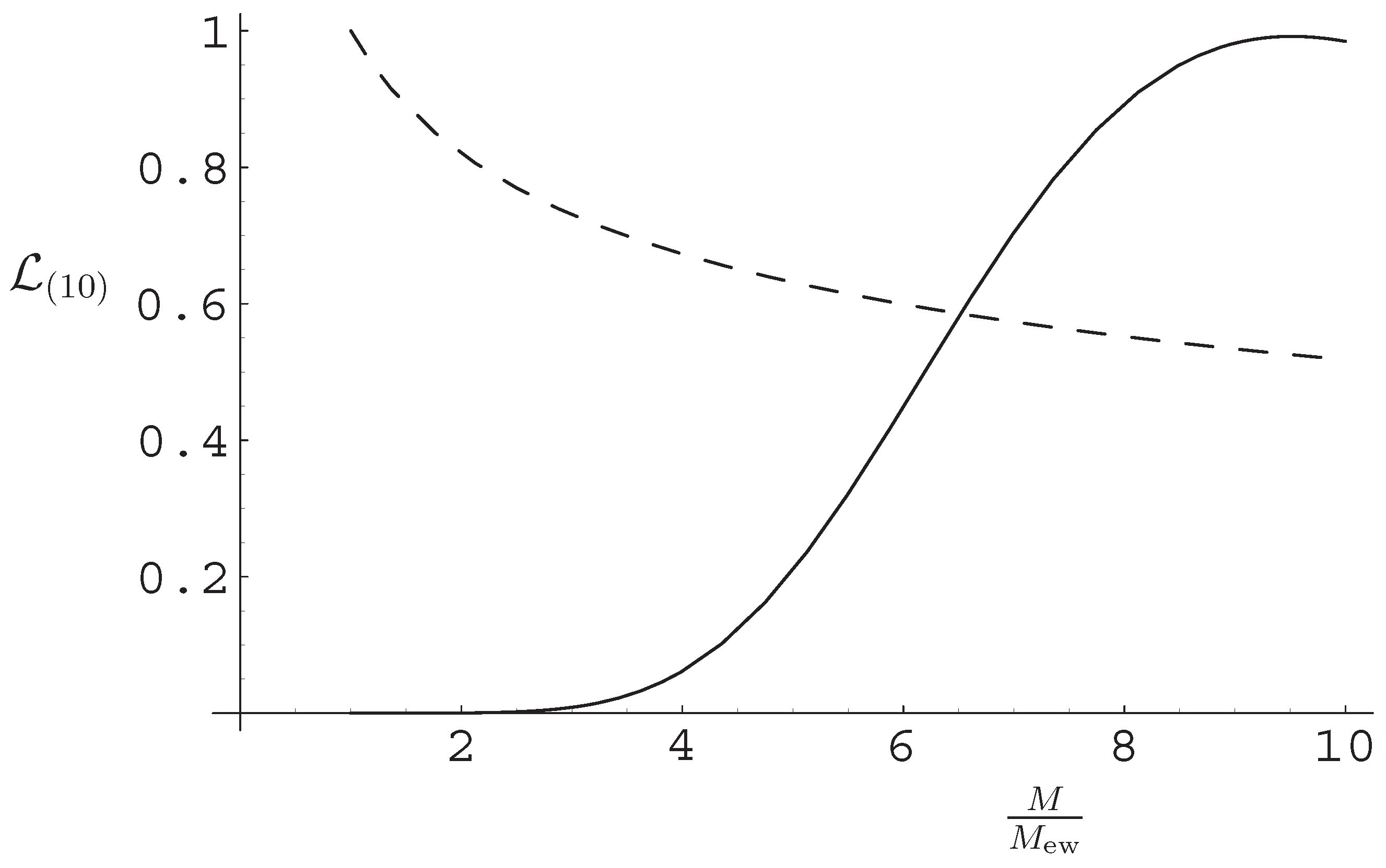
The Euclidean action is of the form in Equation (51) with $M_{\mathrm{eff}}=M_{(4+d)}\sim M_{\mathrm{ew}}$ and $\delta =(d+2)/(d+1)$. In four dimensions one knows that microcanonical corrections to the luminosity become effective only for $M\sim M_{\mathrm{p}}$, therefore, for black holes with $M\gg M_{\mathrm{ew}}$ the luminosity (53) should reduce to the canonical result. In order to eliminate the factor B from Equation (53), one can therefore equate the microcanonical luminosity to the canonical expression at a given reference mass $M_0\gg M_{\mathrm{ew}}$ and then normalize the microcanonical luminosity according to

$$\begin{array}{ccc}\hfill {\mathcal{L}}_{(4+d)}\left(M\right)& \simeq & \frac{{\mathcal{L}}_{(4+d)}^H\left(M_0\right)}{{\mathcal{L}}_{(4+d)}\left(M_0\right)}{\mathcal{L}}_{(4+d)}\left(M\right)\hfill \end{array}$$

(57)

The black hole luminosity thus obtained differs significantly from the canonical one for $M\sim M_{\mathrm{ew}}$, as can be clearly seen from the plot for $d=6$ in Figure 1. For smaller values of d the picture remains qualitatively the same, except that the peak in the microcanonical luminosity shifts to lower values of M. Although the integral in Equation (53) can now be performed exactly, its expression is very complicated and we omit it. In all cases, the microcanonical luminosity becomes smaller for $M\sim M_{\mathrm{ew}}$ than it would be according to the canonical luminosity, which makes the life time of the black hole longer than in the canonical picture [41].

Figure 1. Microcanonical luminosity (solid line) for a small black hole with $d=6$ extra dimensions compared to the corresponding canonical luminosity (dashed line). Vertical units are chosen such that ${\mathcal{L}}_{\left(10\right)}^H\left(M_{\mathrm{ew}}\right)=1$.

Figure 1. Microcanonical luminosity (solid line) for a small black hole with $d=6$ extra dimensions compared to the corresponding canonical luminosity (dashed line). Vertical units are chosen such that ${\mathcal{L}}_{\left(10\right)}^H\left(M_{\mathrm{ew}}\right)=1$.

6.2. RS Scenario

In order to study this case, we shall make use of the solution given in [23],

$$\begin{array}{c}\hfill \mathrm{d}{s}^2=-A\mathrm{d}{t}^2+A^{-1}\mathrm{d}{r}^2+r^2\mathrm{d}{\Omega }^2\end{array}$$

(58)

with

$$\begin{array}{c}\hfill A=1-\frac{2{\ell }_{\mathrm{p}}M}{M_{\mathrm{p}}r}-q\frac{M_{\mathrm{p}}^2{\ell }_{\mathrm{p}}^2}{M_{\left(5\right)}^2{r}^2}\end{array}$$

(59)

where q is the so called tidal charge. For $q>0$, this metric has one horizon at

$$\begin{array}{c}\hfill R_{\mathrm{H}}={\ell }_{\mathrm{p}}\left(\frac{M}{M_{\mathrm{p}}}+\sqrt{\frac{M^2}{M_{\mathrm{p}}^2}+q\frac{M_{\mathrm{p}}^2}{M_{\left(5\right)}^2}}\right)\end{array}$$

(60)

It is then plausible that both the mass M and the (dimensionless) tidal charge q depend upon the black hole proper mass $M_0$ in such a way that when $M_0$ vanishes, so do M and q. The functions $M=M\left(M_0\right)$ and $q=q\left(M_0\right)$ could only be determined precisely by solving the full bulk equations, for example using the four-dimensional metric (58) as a boundary condition. Unfortunately, this task cannot be performed exactly, but only numerically or perturbatively [12,13,14,15,16,17,18,19,20,21,22].

In order to simplify the analysis, we shall first assume that $M=M_0$ and, at least for $M\sim M_{\left(5\right)}$, that the functional form of q is given by

$$\begin{array}{c}\hfill q\simeq {\left(\frac{M_{\mathrm{p}}}{M_{\left(5\right)}}\right)}^{\alpha }{\left(\frac{M}{M_{\left(5\right)}}\right)}^{\beta }\end{array}$$

(61)

where α and $\beta >0$ are real parameters. The luminosity (53) can then be computed exactly and a complete survey is given in [42,43,45]. In general, the decay rate is well-approximated by a power law, namely

$$\begin{array}{c}\hfill {\left.\frac{\mathrm{d}M}{\mathrm{d}\tau }\right|}_{\mathrm{evap}}\simeq C{M}^s\end{array}$$

(62)

where s can be determined analytically for special cases and numerically in general [43].

For instance, let us work out the case with $\beta =1$ and $\delta =1$. The effective four-dimensional Euclidean action is given by

$$\begin{array}{c}\hfill \frac{S_{\left(4\right)}^{\mathrm{E}}}{{\ell }_{\mathrm{p}}{M}_{\mathrm{p}}}\simeq \frac{M}{M_{\mathrm{eff}}}\end{array}$$

(63)

with

$$\begin{array}{c}\hfill M_{\mathrm{eff}}=4M_{\mathrm{p}}\frac{{\ell }_{\mathrm{p}}}{L}\end{array}$$

(64)

and the luminosity in this case is simple enough, that is

$$\begin{array}{c}\hfill \mathcal{L}\simeq B{e}^{-\tilde{M}}\sum _{n=1}^{\infty }\frac{1}{n^4}{\int }_0^{\tilde{M}}{e}^x{\left(\tilde{M}-x\right)}^3\mathrm{d}x\simeq \tilde{B}\end{array}$$

(65)

where we used $M_{\mathrm{eff}}\ll M_{\mathrm{ew}}\sim M$ and $\tilde{B}$ is a new constant. Upon multiplying by the horizon area, we then get the microcanonical evaporation rate per unit proper time

$$\begin{array}{c}\hfill {\left.\frac{\mathrm{d}M}{\mathrm{d}\tau }\right|}_{\mathrm{evap}}\simeq CM\end{array}$$

(66)

where C is again a constant we can determine by equating the rate (66) with the Hawking expression (55) for $M=M_{\mathrm{c}}$ defined by $R_{\mathrm{H}}\left(M_{\mathrm{c}}\right)\simeq L$.

7. Summary

We have reviewed the main arguments in favor of the microcanonical ensemble for describing evaporating black holes. A shortcoming of the foregoing analysis is the use of the mean field approximation. However, all calculations of particle emission utilize this approximation, and the microcanonical approach is clearly preferable to the thermodynamical approach in the semiclassical quantization processes described above. It is free of the inconsistencies present in the thermodynamical approach, and its predictions seem to be more physically reasonable, e.g., a finite black hole decay rate throughout the life of the black hole. The use of a fixed energy basis for the Hilbert space of the theory instead of the usual thermal state implies that black holes are particle states. In our interpretation of black holes as quantum objects the associated quantum degeneracy of states obtained from the inverse of the tunneling probability points to the identification of black holes with the excitation modes of p-branes.

For a four-dimensional black hole the above picture leads to very small, undetectable, departures from the usual Hawking picture. However, if extra dimensions exist, and the fundamental scale of quantum gravity is as low as $1$TeV, microscopic black holes with a mass of a few TeV’s might be produced in modern accelerators. In this case the microcanonical description then becomes a necessary tool to describe their evaporation, and there is no need for the thermodynamical concept of entropy for microscopic black holes. In general, one then expects an increased life time with respect to what would be predicted by the canonical ensemble, with the ending stage of the evaporation resembling a more conventional, quasi-exponential decay. For more details on the phenomenological signatures of microscopic black holes at the LHC in the microcanonical treatment, we just refer the reader to [52,53,71].

References

- Harms, B.; Leblanc, Y. Statistical mechanics of black holes. Phys. Rev. D 1992, 46, 2334–2340. [Google Scholar] [CrossRef]
- Harms, B.; Leblanc, Y. Statistical mechanics of extended black objects. Phys. Rev. D 1993, 47, 2438–2445. [Google Scholar] [CrossRef]
- Harms, B.; Leblanc, Y. Complete semiclassical treatment of the quantum black hole problem. Ann. Phys. 1995, 244, 262–271. [Google Scholar] [CrossRef]
- Harms, B.; Leblanc, Y. Proper field quantization in black hole space-times. Ann. Phys. 1995, 244, 272–282. [Google Scholar] [CrossRef]
- Cox, P.H.; Harms, B.; Leblanc, Y. Dilatonic black holes, naked singularities and strings. Europhys. Letts. 1994, 26, 321–326. [Google Scholar] [CrossRef]
- Harms, B.; Leblanc, Y. Black extended objects, naked singularities and P-branes. Europhys. Letts. 1994, 27, 557–562. [Google Scholar] [CrossRef]
- Harms, B.; Leblanc, Y. Conjectures on nonlocal effects in string black holes. Ann. Phys. 1995, 242, 265–274. [Google Scholar] [CrossRef]
- Casadio, R.; Harms, B.; Leblanc, Y. Statistical mechanics of Kerr-Newman dilaton black holes and the bootstrap condition. Phys. Rev. D 1998, 57, 1309–1312. [Google Scholar] [CrossRef]
- Casadio, R.; Harms, B.; Leblanc, Y. Microfield dynamics of black holes. Phys. Rev. D 1998, 58, 044014. [Google Scholar] [CrossRef]
- Cavaglia, M. Black hole and brane production in TeV gravity: A Review. Int. J. Mod. Phys. A 2003, 18, 1843–1882. [Google Scholar] [CrossRef]
- Kanti, P. Black holes in theories with large extra dimensions: A Review. Int. J. Mod. Phys. A 2004, 19, 4899–4951. [Google Scholar] [CrossRef]
- Whisker, R. Braneworld black holes. arXiv, 2008; arXiv:0810.1534, [gr-qc]. [Google Scholar]
- Gregory, R. Braneworld black holes. Lect. Notes Phys. 2009, 769, 259–298. [Google Scholar]
- Emparan, R.; Horowitz, G.T.; Myers, R.C. Exact description of black holes on branes. JHEP 2000, 0001, 007. [Google Scholar] [CrossRef]
- Shiromizu, T.; Shibata, M. Black holes in the brane world: Time symmetric initial data. Phys. Rev. D 2000, 62, 127502. [Google Scholar] [CrossRef]
- Chamblin, A.; Reall, H.S.; Shinkai, H.-a.; Shiromizu, T. Charged brane world black holes. Phys. Rev. D 2001, 63, 064015. [Google Scholar] [CrossRef]
- Casadio, R.; Fabbri, A.; Mazzacurati, L. New black holes in the brane world? Phys. Rev. D 2002, 65, 084040. [Google Scholar] [CrossRef]
- Kanti, P.; Tamvakis, K. Quest for localized 4-D black holes in brane worlds. Phys. Rev. D 2002, 65, 084010. [Google Scholar] [CrossRef]
- Kudoh, H.; Tanaka, T.; Nakamura, T. Small localized black holes in brane world: Formulation and numerical method. Phys. Rev. D 2003, 68, 024035. [Google Scholar] [CrossRef]
- Casadio, R.; Mazzacurati, L. Bulk shape of brane world black holes. Mod. Phys. Lett. A 2003, 18, 651–660. [Google Scholar] [CrossRef]
- Creek, S.; Gregory, R.; Kanti, P.; Mistry, B. Braneworld stars and black holes. Class. Quant. Grav. 2006, 23, 6633–6658. [Google Scholar] [CrossRef]
- Dai, D.C.; Stojkovic, D. Analytic solution for a static black hole in RSII model. arXiv, 2010; arXiv:1004.3291, [gr-qc]. [Google Scholar]
- Dadhich, N.; Maartens, R.; Papadopoulos, P.; Rezania, V. Black holes on the brane. Phys. Lett. B 2000, 487, 1–6. [Google Scholar] [CrossRef]
- Arkani-Hamed, N.; Dimopoulos, S.; Dvali, G.R. The Hierarchy problem and new dimensions at a millimeter. Phys. Lett. B 1998, 429, 263–272. [Google Scholar] [CrossRef]
- Arkani-Hamed, N.; Dimopoulos, S.; Dvali, G.R. Phenomenology, astrophysics and cosmology of theories with submillimeter dimensions and TeV scale quantum gravity. Phys. Rev. D 1999, 59, 086004. [Google Scholar] [CrossRef]
- Antoniadis, I.; Arkani-Hamed, N.; Dimopoulos, S.; Dvali, G.R. New dimensions at a millimeter to a Fermi and superstrings at a TeV. Phys. Lett. B 1998, 436, 257–263. [Google Scholar] [CrossRef]
- Randall, L.; Sundrum, R. An Alternative to compactification. Phys. Rev. Lett. 1999, 83, 4690–4693. [Google Scholar] [CrossRef]
- Argyres, P.C.; Dimopoulos, S.; March-Russell, J. Black holes and submillimeter dimensions. Phys. Lett. B 1998, 441, 96–104. [Google Scholar] [CrossRef]
- Dimopoulos, S.; Landsberg, G.L. Black holes at the LHC. Phys. Rev. Lett. 2001, 87, 161602. [Google Scholar] [CrossRef] [PubMed]
- Giddings, S.B.; Thomas, S.D. High-energy colliders as black hole factories: The end of short distance physics. Phys. Rev. D 2002, 65, 056010. [Google Scholar] [CrossRef]
- Harris, C.M.; Richardson, P.; Webber, B.R. CHARYBDIS: A Black hole event generator. JHEP 2003, 0308, 033. [Google Scholar] [CrossRef]
- Alberghi, G.L.; Casadio, R.; Tronconi, A. Quantum gravity effects in black holes at the LHC. J. Phys. G 2007, 34, 767–778. [Google Scholar] [CrossRef]
- Cavaglia, M.; Godang, R.; Cremaldi, L.; Summers, D. Catfish: A Monte Carlo simulator for black holes at the LHC. Comput. Phys. Commun. 2007, 177, 506–517. [Google Scholar] [CrossRef]
- Dai, D.C.; Starkman, G.; Stojkovic, D.; Issever, C.; Rivzi, E.; Tseng, J. BlackMax: A black-hole event generator with rotation, recoil, split branes, and brane tension. Phys. Rev. D 2008, 77, 076007. [Google Scholar] [CrossRef]
- Frost, J.A.; Gaunt, J.R.; Sampaio, M.O.P.; Casals, M.; Dolan, S.R.; Parker, M.A.; Webber, B.R. Phenomenology of production and decay of spinning extra-dimensional black holes at hadron colliders. JHEP 2009, 0910, 014. [Google Scholar] [CrossRef]
- Gingrich, D.M. Quantum black holes with charge, colour, and spin at the LHC. J. Phys. G 2010, 37, 105108. [Google Scholar] [CrossRef]
- Gingrich, D.M. Production of tidal-charged black holes at the Large Hadron Collider. Phys. Rev. D 2010, 81, 057702. [Google Scholar] [CrossRef]
- Casadio, R.; Nicolini, P. The decay-time of non-commutative micro-black holes. JHEP 2008, 0811, 072. [Google Scholar] [CrossRef]
- Casadio, R.; Harms, B. Black Hole Evaporation and Compact Extra Dimensions. Phys. Rev. D 2001, 64, 024016. [Google Scholar] [CrossRef]
- Casadio, R.; Harms, B. Black hole evaporation and large extra dimensions. Phys. Lett. B 2000, 487, 209–214. [Google Scholar] [CrossRef]
- Casadio, R.; Harms, B. Can black holes and naked singularities be detected in accelerators? Int. J. Mod. Phys. A 2002, 17, 4635–4646. [Google Scholar] [CrossRef]
- Casadio, R.; Fabi, S.; Harms, B. Possibility of catastrophic black hole growth in the warped brane-world scenario at the LHC. Phys. Rev. D 2009, 80, 084036. [Google Scholar] [CrossRef]
- Casadio, R.; Fabi, S.; Harms, B.; Micu, O. Theoretical survey of tidal-charged black holes at the LHC. JHEP 2010, 1002, 079. [Google Scholar] [CrossRef]
- Casadio, R.; Micu, O. Exploring the bulk of tidal charged micro-black holes. Phys. Rev. D 2010, 81, 104024. [Google Scholar] [CrossRef]
- Casadio, R.; Harms, B.; Micu, O. Effect of brane thickness on microscopic tidal-charged black holes. Phys. Rev. D 2010, 82, 044026. [Google Scholar] [CrossRef]
- Bekenstein, J.D. Black holes and entropy. Phys. Rev. D 1973, 7, 2333–2346. [Google Scholar] [CrossRef]
- Bekenstein, J.D. Generalized second law of thermodynamics in black hole physics. Phys. Rev. D 1974, 9, 3292–3300. [Google Scholar] [CrossRef]
- Bardeen, J.M.; Carter, B.; Hawking, S.W. The four laws of black hole mechanics. Commun. Math. Phys. 1973, 31, 161–170. [Google Scholar] [CrossRef]
- Chavanis, P.H. Phase transitions in self-gravitating systems. Int. J. Mod. Phys. B 2006, 20, 3113–3198. [Google Scholar] [CrossRef]
- Hawking, S.W. Particle creation by black holes. Comm. Math. Phys. 1975, 43, 199–220. [Google Scholar] [CrossRef]
- Gibbons, G.W.; Hawking, S.W. Action integrals and partition functions in quantum gravity. Phys. Rev. D 1977, 15, 2752–2756. [Google Scholar] [CrossRef]
- Hossenfelder, S.; Bleicher, M.; Hofmann, S.; Stoeker, H.; Kotval, A.V. Black hole relics in large extra dimensions. Phys. Lett. B 2003, 566, 233–239. [Google Scholar] [CrossRef]
- Koch, B.; Bleicher, M.; Hossenfelder, S. Black hole remnants at the LHC. JHEP 2005, 0510, 053. [Google Scholar] [CrossRef]
- Scardigli, F.; Gruber, C.; Chen, P. Black hole remnants in the early universe. arXiv, 2010; arXiv:1009.0882, [gr-qc]. [Google Scholar]
- Nicolini, P. Noncommutative black holes, the final appeal to quantum gravity: A review. Int. J. Mod. Phys. A 2009, 24, 1229–1308. [Google Scholar] [CrossRef]
- Parikh, M.K.; Wilczek, F. Hawking radiation as tunneling. Phys. Rev. Lett. 2000, 85, 5042–5045. [Google Scholar] [CrossRef] [PubMed]
- Parikh, M.K. A Secret tunnel through the horizon. Int. J. Mod. Phys. D 2004, 13, 2351–2354. [Google Scholar] [CrossRef]
- Myers, R.C.; Perry, M.J. Black holes in higher dimensional space-times. Annals Phys. 1986, 172, 304. [Google Scholar] [CrossRef]
- Fubini, S.; Hanson, A.J.; Jackiw, R. New approach to field theory. Phys. Rev. D 1973, 7, 1732–1760. [Google Scholar] [CrossRef]
- Dethlefsen, J.; Nielsen, H.B.; Tze, H.C. The hagedorn spectrum distribution and the dimension of hadronic matter. Phys. Lett. B 1974, 48, 48–50. [Google Scholar] [CrossRef]
- Strumia, A.; Venturi, G. Are hadrons strings? Lett. Nuovo Cimento 1975, 13, 337. [Google Scholar] [CrossRef]
- Umezawa, H.; Matsumoto, H.; Tachiki, M. Thermo Field Dynamics and Condensed States; North-Holland Publishing Co.: Amsterdam, The Netherland, 1982. [Google Scholar]
- Hagedorn, R. Statistical thermodynamics of strong interactions at high-energies. Nuovo Cimento Suppl. 1965, 3, 147–186. [Google Scholar]
- Frautschi, S.C. Statistical bootstrap model of hadrons. Phys. Rev. D 1971, 3, 2821–2834. [Google Scholar] [CrossRef]
- Carlitz, R.D. Hadronic matter at high density. Phys. Rev. D 1972, 5, 3231–3242. [Google Scholar] [CrossRef]
- Kubo, R. Statistical Mechanics; Norht-Holland Publishing Co.: Amsterdam, The Netherland, 1980. [Google Scholar]
- Leblanc, Y. Statistical field dynamics. Unpublished material. Available online: http://www.efieldtheory.com/articles/?eFTC=020701 (accessed on 1 September 2010).
- Birrell, N.D.; Davies, P.C.W. Quantum Fields in Curved Space; Cambridge University Press: Cambridge, UK, 1982. [Google Scholar]
- Carr, B.J.; MacGibbon, J.H. Cosmic rays from primordial black holes and constraints on the early universe. Phys. Rept. 1998, 307, 141–154. [Google Scholar] [CrossRef]
- Kotwal, A.V.; Hofmann, S. Discrete energy spectrum of Hawking radiation from Schwarzschild surfaces. arXiv, 2002; [hep-ph/0204117]. [Google Scholar]
- Gingrich, D.M.; Martell, K. Microcanonical treatment of black hole decay at the Large Hadron Collider. J. Phys. G Nucl. Part. Phys. 2008, 35, 035001. [Google Scholar] [CrossRef]
© 2011 by the authors; licensee MDPI, Basel, Switzerland. This article is an open access article distributed under the terms and conditions of the Creative Commons Attribution license (http://creativecommons.org/licenses/by/3.0/.)
Share and Cite
MDPI and ACS Style
Casadio, R.; Harms, B. Microcanonical Description of (Micro) Black Holes. Entropy 2011, 13, 502-517. https://doi.org/10.3390/e13020502
AMA Style
Casadio R, Harms B. Microcanonical Description of (Micro) Black Holes. Entropy. 2011; 13(2):502-517. https://doi.org/10.3390/e13020502
Chicago/Turabian StyleCasadio, Roberto, and Benjamin Harms. 2011. "Microcanonical Description of (Micro) Black Holes" Entropy 13, no. 2: 502-517. https://doi.org/10.3390/e13020502