Article

Information Theory and Dynamical System Predictability

Courant Institute of Mathematical Sciences, New York University, 251 Mercer Street, New York, NY 10012, USA
Entropy 2011, 13(3), 612-649; https://doi.org/10.3390/e13030612
Submission received: 25 January 2011 / Revised: 14 February 2011 / Accepted: 20 February 2011 / Published: 7 March 2011
(This article belongs to the Special Issue Advances in Information Theory)

Abstract

:
Predicting the future state of a turbulent dynamical system such as the atmosphere has been recognized for several decades to be an essentially statistical undertaking. Uncertainties from a variety of sources are magnified by dynamical mechanisms and given sufficient time, compromise any prediction. In the last decade or so this process of uncertainty evolution has been studied using a variety of tools from information theory. These provide both a conceptually general view of the problem as well as a way of probing its non-linearity. Here we review these advances from both a theoretical and practical perspective. Connections with other theoretical areas such as statistical mechanics are emphasized. The importance of obtaining practical results for prediction also guides the development presented.

Graphical Abstract

1. Introduction

Prediction within dynamical systems originated within the modern era in the study of the solar system. The regularity of such a system on time scales of centuries meant that very precise predictions of phenomena such as eclipses are possible at such lead times. On longer times scales of order million or more years, chaotic behavior due to the multi-body gravitational interaction becomes evident (see e.g., [1]) and effects such as planetary collisions or system ejection can occur. Naturally at such leads where chaotic behavior dominates predictions become far less precise. Of course, predictions over such a timescale are only theoretical and not subject to observational verification.
In the last century prediction within a greater range of practical dynamical systems has been attempted. Perhaps the best known of these have been turbulent fluids such as the atmosphere and ocean as well as earthquake prediction for which the system can be considered even more non-linear. It is fair to say that considerable progress has been made in the first area; the second area has potential currently limited by a lack of observations while in the third area more limited success has been achieved (see e.g., [2]).
Predictions made using a dynamical model typically suffer primarily from two deficiencies: Firstly the model used may have certain inadequacies as a representation of reality and secondly initial conditions for a prediction may not be known exactly. Such problems are known as model errors and initial condition errors respectively. Uncertainty in boundary conditions can sometimes be of importance as well. We omit a discussion of this effect in the present review.
Progress can be made in improving predictions either by improving physical depictions within models or by improving the observational network and thereby reducing errors in the initial conditions. There is considerable evidence for the atmosphere however that no practical observational network will ever eliminate significant prediction errors due to initial condition errors. Even if one was able to define such conditions to the round-off accuracy of the computing device deployed, at some practical prediction time even these minute errors would grow sufficiently large as to overwhelm the forecast made. Such behavior is of course characteristic of dynamical systems classified loosely as chaotic or turbulent.
In general model errors are almost by definition quite hard to study in a systematic fashion since they are caused by quite diverse factors which are not very well understood. In fact if they were better understood they would be removed by improving the dynamical model using this knowledge. Thus the issue of model error tends primarily to be an engineering rather than a theoretical study. We therefore focus our attention here on initial condition errors but it should be borne in mind that model errors can often cause substantial problems for forecasters. It is interesting that the general public often confuses the two issues and attributes errors due to initial condition uncertainty to the inadequacy of meteorologists in reducing model errors. Of course meteorologists are not always averse to using the reverse strategy in response.
Inevitable deficiencies in observing networks imply uncertainty about the initial conditions used in predictions which can therefore be considered random variables. The study of the evolution of such variables thus in a general sense can be considered to be the study of predictability. Naturally functionals connected with uncertainty defined on such variables play an important role in such studies. In the context of atmospheric prediction, most attention has focused on the first two moments of the associated probability functions since often such functions are quasi-normal. Study of the problems from the viewpoint of entropic functionals is the natural generalization of this which allows for a more general treatment and this has received considerable attention in the last decade and is the subject of this review.
The dynamical systems of practical interest are generally of rather high dimensionality and this has posed particular problems for predictability studies. It means that study of the evolution of the multivariate probability distribution is generally impossible and studies are often confined to Monte Carlo (ensemble) predictions. The size of such ensembles are usually far less than the system dimensionality which has led to a wide variety of reduced state space techniques for identifying important error growth directions. Related reduced state space methods can also be used to truncate the dynamical system to a stochastically forced low order system. Such reductions have proved very useful in illuminating dominant dynamical processes and may also be amenable to complete analytical solution.
With regard to predictability studies, the functionals which have been studied most are differential entropy, information divergence and mutual information. This second is also commonly called the Kullback-Leibler divergence and the relative entropy. We use the terminology information divergence or just divergence to distinguish it clearly from the usual entropy. The dynamical evolutions of the first two are of particular interest with the second being defined with respect to the time evolving probability distribution and the equilibrium (climatological) probability distribution of the system. In general these two distributions converge with time and when they are statistically indistinguishable in some sense (to be made precise below) all predictability has been lost. Indeed an illuminating way to view predictability is as a measure of the disequilibrium of a statistical system. All this is discussed further in Section 2, Section 3 and Section 5 below.
The review is structured as follows: The next section is a brief review of the mostly well known properties of the relevant entropic functionals to be discussed. Section 3 discusses general entropic evolution equations in dynamical systems for which the generic Chapman Kolmogorov equation is relevant. Several of these results are not new but all of the material is not widely known outside statistical physics. Section 4 discusses the concept of information (uncertainty) flow within a dynamical system and its applications. Section 5 discusses various approaches to the study of predictability using the previous tools and outlines a number of new results obtained in the last decade. Finally Section 6 draws some general conclusions on work to date and potential future directions.
The approach taken in this review is slanted toward the authors and co-workers work in this area but other perspectives are also outlined and referenced. In general the nature of this work is rather eclectic given the attempt to balance the theoretical with the practical. It is hoped there will be materials here of interest to a rather broad audience. The intention is to connect information theoretic approaches to predictability with the broad area of statistical physics. A different approach to this subject which emphasizes more geophysical applications may be found in the excellent review of [3]. Other more theoretical approaches may be found in [4] and [5]. We have also chosen in the interests of brevity to omit the treatment of data assimilation and data filters from an information theoretic perspective but remind the reader that there is significant effort in that area as well (see, for example, [6] and [7]).

2. Relevant Information Theoretic Functionals and Their Properties

Results quoted without proof may be found in [8]. Consider two vector random variables X and Y with associated countable outcome alphabet A and associated probability functions p ( x ) and q ( x ) with x A . The entropy or uncertainty is defined by
H ( X ) x A p ( x ) log 1 p ( x )
which is obviously non-negative. The (information) divergence between X and Y is defined by
D ( p | | q ) x A p ( x ) log p ( x ) q ( x )
This is also non-negative and only vanishes when p = q so can be considered a “distance” function between functions although it is neither symmetric nor satisfies the triangle identity of Euclidean distance. In the limit that the two probability functions are “close” then indeed it does satisfy these identities to arbitrary accuracy. This is an indication that the divergence induces a metric structure in the sense of differential geometry on the space of probability densities. Further discussion can be found in [9].
If we concatenate X and Y then we can define a joint probability function p ( x , y ) with associated marginal distributions p ( x ) and p ( y ) . The mutual information then measures the “distance” between this joint distribution and one for which X and Y are independent i.e., p ( x , y ) = p ( x ) p ( y ) . Thus we have
I ( X ; Y ) D ( p ( x , y ) | | p ( x ) p ( y ) ) = x , y A p ( x , y ) log p ( x , y ) p ( x ) p ( y )
Given its definition, the mutual information represents the degree of dependency between different random variables. Finally we can use the joint distribution p ( x , y ) to define the conditional entropy H ( X | Y ) as the expected uncertainty in X given that Y is known precisely.
The entropic functionals defined above can be generalized to so called differential entropic functionals defined on random variables with continuous alphabets. It is interesting however to attempt to interpret them as limits of their countable analogs. Thus for example the differential entropy h ( X ) is defined as:
h ( X ) S p ( x ) log ( p ( x ) ) d x
where S is the continuous outcome set for X . If we convert this to a Riemann sum we obtain
h ( X ) i Λ p ( x i * ) log ( p ( x i * ) ) Δ = i Λ P i log P i + log Δ = H ( X ˜ ) + log Δ
where Δ is the (assumed constant) volume element for the Riemann sum partitioning Λ chosen. Clearly as this approaches zero, the second term approaches and the differential entropy is finite only because H ( X ˜ ) diverges to + . This latter divergence occurs because the larger the size of the index/alphabet set Λ the larger the entropy since there is increased choice in outcomes. One can overcome this rather awkward limiting process by restricting attention to entropy differences of different random variables in which case the log Δ term cancels.
By contrast the “differential” divergence is a straightforward limit of the ordinary divergence:
D ( p | | q ) S p ( x ) log ( p ( x ) / q ( x ) ) d x i Λ p ( x i * ) log ( p ( x i * ) / q ( x i * ) ) Δ = i Λ P i log ( P i / Q i ) = D ( P | | Q )
Note the cancellation of Δ in the third expression here.
This cancellation effect is also important to the transformational properties of the differential functionals. In particular suppose we have the following general non-linear change of variables:
y = r ( x )
The transformed probability density p ( y ) is well known to be given by
p ( y ) = p ( r 1 ( y ) ) det r 1 ( y ) y
and the change of variables formula for integration has it that
d x = d y det r 1 ( y ) y d y det J
where J is the so-called Jacobian of the transformation. So we have
D ( p | | q ) = S p ( y ) log ( p ( y ) / q ( y ) ) d y = S p ( x ) log ( p ( x ) det J / q ( x ) det J ) d x = D ( p | | q )
providing the determinant of the transformation does not vanish which is a condition for the non-singularity of the transformation. Notice that this proof does not work for the differential entropy because of the lack of cancellation. The difference of the differential entropy of two random variables will be invariant under affine transformations because then det J is constant and the integral of the probability density is also constant (unity). For an affine transformation of the form
x = A x + c
where the matrix A and vector c are constant one can easily establish in using the similar arguments to above that
h ( A X ) = h ( X ) + log det A
Notice that this equation also implies that new distributions that are given by
p ( x ) = p ( x )
have the same differential entropy providing that the affine transformation is volume preserving i.e., det A = ± 1 . Note however that in general D ( p | | p ) will be non-zero and positive unless the probability distribution has a symmetry under the transformation.
In addition to the above general transformational invariance and straightforward limiting property, the divergence also satisfies an intuitive fine graining relationship. Thus if one subdivides a particular partitioning Λ into a finer partitioning Λ then one can easily establish (using the log sum inequality) that the divergence defined on the new partition is at least as large as the original coarse grained functional. Thus if the limit to the continuous functional is taken in this fine graining fashion then the divergence converges monotonically to the continuous limit. This has the intuitive interpretation that as finer and finer scales are considered, that “differences” in probability functions become larger as finer structure is used to make the assessment of this “difference”.

3. Time Evolution of Entropic Functionals

We begin our discussion within the context of a general stochastic process. A well known result from information theory called the generalized second law of thermodynamics states that under certain conditions the divergence is a non-increasing function of time. We formulate this in terms of causality.
Definition 1. 
Suppose we have two stochastic processes X ( t ) and Y ( t ) with t R denoting time and associated probability functions p and q the same outcome sets x ( t ) . We say that the two processes are causally similar if
p x ( t ) | x ( t a ) = q x ( t ) | x ( t a ) x t R a n d a > 0
This condition expresses intuitively the notion that the physical system giving rise to the two processes is identical and that precise knowledge of the set of values for outcomes at a particular time are sufficient to determine the future evolution of probabilities. This is intuitively the case for a closed physical system however not the case for an open system since in this second case other apparently external variables may influence the dynamical evolution. Note that the condition of probabilistic causality (7) introduces an arrow in time (via the restriction a > 0 ). Also note that a time-homogeneous Markov process satisfies this condition.
It is now easy to show that the divergence of two causally similar processes is non-increasing (the proof can be found in [8]). In some systems referred to as reversible (see below) this functional will actually be conserved while in others termed irreversible, it will exhibit a strict decline. Note that this result applies to all causally similar processes but often one is taken to be the equilibrium process and in irreversible processes the divergence then measures the degree of equilibration of the system.
Consider now a continuous time continuous state Markov process governed by the well known (see e.g., [10]) Fokker Planck equation (FPE):
t p = i = 1 N i A i ( x , t ) p + 1 2 i , j = 1 N i j B ( x , t ) B t ( x , t ) i j p
C i j B ( x , t ) B t ( x , t ) i j n o n n e g a t i v e d e f i n i t e
where A i and C i j are respectively referred to as the drift vector and diffusion tensor. We can derive a series of interesting results regarding the time evolution of both differential entropy and divergence. Detailed proofs may be found in the Appendix. The first result is well known in statistical physics and dynamical systems studies (see, for example, [11] and [12]).
Theorem 2. 
Suppose we have a stochastic process obeying Equation (8) with B = 0 and associated probability function f then the ordinary (differential) entropy satisfies the evolution equation
h t = f A d x = A f
Notice the importance of A to the entropy evolution. This also measures the rate at which an infinitesimal volume element expands or contracts in the dynamical system. When it vanishes the system is sometimes said to satisfy a Liouville condition. Hamiltonian systems which includes many inviscid (frictionless) fluids satisfy such a condition. We shall use Equation (10) in a central way in the next section when we consider the concept of information flow.
A particular instructive case when A < 0 occurs in the case of dissipative systems. A damped linear system has this quantity as a negative constant. In such a case the entropy declines since all trajectories end in the same fixed point. In the case that the system has some stochastic forcing and so the diffusion term in the Fokker Planck equation does not vanish then the stochastic forcing generally acts to increase entropy as the following extension shows:
Theorem 3. 
Suppose we have a general stochastic process with probability function p governed by a Fokker Planck equation which is restricted by the stochastic forcing condition
i C i j = 0
where we are assuming the summation convention. Then the evolution of the differential entropy is given by the equation
h t = A p + 1 2 C i j i log p j log p p
The second term here clearly results in no decline in entropy given that C i j is non-negative definite.
In the case of a stochastically forced dissipative system it is possible for the system to reach an equilibrium where the entropy creation due to the stochastic forcing is balanced by its destruction via the dissipative deterministic dynamics. This balance is an example of a fluctuation dissipation result. A particular case of this theorem with C i j constant was stated in [11] and the two terms on the right hand side of (12) were referred to as entropy production and entropy flux respectively. Also within this reference there is a discussion of the relationship of this type of entropy evolution equation to others proposed in statistical physics using Lyapunov exponents (e.g., [13]).
In contrast to the evolution of differential entropy, the divergence is conserved in all systems even dissipative ones providing B = 0 :
Theorem 4. 
Suppose we have two stochastic processes obeying Equation (8) which have the additional condition that B ( x , t ) = 0 then the divergence of the two processes (if defined) is time invariant.
In many dynamical systems with B = 0 if one calculates the divergence with respect to a particular finite partitioning of state space rather than in the limit of infinitesimal partitioning then the conservation property no longer holds and in many interesting cases it declines with time instead and the system equilibrates. This reflects the fact that as time increases the difference in the distributions tends to occur on the unresolved scales which are not measured by the second divergence calculation. Such a coarse graining effect is of course the origin of irreversibility and often the “unresolved” scales are modeled via a stochastic forcing i.e., we set B 0 . In such a case we get a strict decline with time of divergence. The following result was due originally to [14], the proof here follows [15]
Theorem 5. 
Suppose we have two distinct (i.e. differing on a set of measure greater than zero) stochastic processes obeying (8) with C = B ( x , t ) B t ( x , t ) positive definite almost everywhere and with associated probability densities f and g then the divergence strictly declines and satisfies the evolution equation
D ( f | | g ) t = C i j i log ( f / g ) j log ( f / g ) f
This final theorem shows the central role of stochastic forcing in causing divergence to decline and hence to the modeling of irreversibility. In the context of statistical physics, the non-positive term on the right hand side of (13) with g set to the equilibrium distribution (invariant measure) forms a part of discussions on non-equilibrium entropy production (see [11]).
In stochastic modeling of dynamical systems it is common to separate the state space into fast and slow components and model the former with noise terms and dissipation of the slow modes. Presumably in this case if such a model works well as a coarse grained model for the total unforced and undissipated system then the last two theorems imply that there is a “leakage” of divergence from the slow to the fast components of the system.
It is an empirical fact that in many physical systems of interest, we find that if a slow subspace is chosen which represents a large fraction of the variability of the system then the subspace divergence will always show a monotonic decline which is suggestive that stochastic models of this system may work well. In the more general dynamical system context however it is an interesting question under what circumstances the fine scales can cause an increase in the divergence with respect to the coarse scales. After all the coarse grained system is not closed and so the monotonicity result quoted at the beginning of this section need not necessarily apply. Related questions have rather naturally generated considerable interest in the statistical physics literature since they relate to the fundamental issue of temporal direction. There is a vast literature and interested readers are referred to, for example, [16,17,18] and [19] Chapter 5.
It is possible to extend the Fokker Planck equation to include discontinuous jump processes and then this equation becomes the more general (differential) Chapman-Kolmogorov equation. The additional terms are often referred to (on their own) as the master equation. It is then possible by similar arguments to those given above to conclude that the jump processes result in an additional strict monotonic decline in divergence. The interested reader is referred to Chapter 3 of [15] for a sketch proof and more information and references.
There is also a well known connection between these results and the classical kinetic theory of Boltzmann which applies to dilute gases. In the latter case the probability distribution of molecules in the absence of collisions is controlled by an equation identical to the Fokker Planck equation with B = 0 . The molecules themselves are controlled by a Hamiltonian formulation which means that the probability equation can be shown to also satisfy A = 0 . Thus both the entropy and divergence are conserved. Collisions between molecules are modeled probabilistically using a hypothesis known as the Stosszahlansatz or molecular chaos hypothesis (see [20] p. 375). This amounts to the insertion of master equation terms and so the resulting Boltzmann equation can be viewed as a Chapman Kolmogorov equation. The particular form of the master equation ensures that both divergence and differential entropy satisfy monotonic declines and increases respectively. This result is known as Boltzmann’s H-theorem and is the traditional origin of irreversibility in statistical mechanics. More detail can be found in standard treatments of statistical mechanics.
In the context of inviscid fluid turbulence there has been considerable interest in the establishment of H-theorems (see e.g., [21,22,23] and references cited therein). A revealing and conceptually powerful way in which such turbulence can be effectively coarse-grained (and hence simplified) is through moment closures such as eddy-damped Markovian methods (see [24]). This is basically equivalent to the stochastic modeling of the fluid (see [25] Chapter 5) in the manner considered above. Interestingly when this particular kind of coarse-graining is performed one is able to establish rigorously that entropy monotonically increases as a fluid approaches statistical equilibrium (see [21]). It is worth re-emphasizing that this state of affairs is not necessarily guaranteed in more general systems for which Equation (12) applies.

4. Information Flow

4.1. Theory

If we partition a closed dynamical system then an interesting question arises regarding the evolution of uncertainty within the subsets chosen. How does it depend on the evolution of the other partitions? In general as we saw in the last section, entropy is not conserved globally unless the Liouville property holds, so the flow of uncertainty within a system does not usually follow the standard continuity equation satisfied by quantities such as energy, charge or mass. This concept of uncertainty flow has some important practical applications since it is clear that reduction of uncertainty in one partition member at a particular time may depend importantly on the reduction of uncertainty in another partition member at an earlier time. Clearly then understanding the flow of uncertainty is potentially important to optimizing predictions.
This issue was first addressed by [26] who studied the propagation of perturbations in simple non-linear dynamical systems using a “moving frame” or co-moving Lyupanov exponent defined by
λ ( v ; x 1 , x 2 ) lim t 1 t ln Δ ( v , x 1 , x 2 , t ) Δ ( v , x 1 , x 2 , 0 )
where perturbation amplitudes Δ are defined using an L 2 norm on a moving interval:
Δ ( v , x 1 , x 2 , t ) x 1 + v t x 2 + v t δ ψ ( x , t ) 2 d x 1 2
with respect to small deviations in the system variables ψ ( x , t ) . Maximization of this with respect to the moving frame velocity v showed the preferred velocity of growing perturbations. Since regular Lyupanov exponents are often related to entropy production it was natural to try to find an information theoretic counterpart for the co-moving exponents. This turned out empirically and in the systems studied, to be the time lagged mutual information (TLMI) of random variables I ( X ( t 1 ) ; Y ( t 2 ) ) where the random variables are located at different spatial locations. Associated with the TLMI is the natural velocity scale
v d ( X , Y ) t 2 t 1
where d is the spatial distance between the random variables. The TLMI turned out to be maximized when this velocity matched that which maximized the co-moving Lyupanov exponent.
In addition to this match of physical propagation scales, mutual information has an appealing interpretation as the reduction in uncertainty of X ( t 1 ) due to perfect knowledge of Y ( t 2 ) i.e., roughly speaking, the contribution of uncertainty in the former due to uncertainty in the latter. This follows from the identity
I ( X ( t 1 ) ; Y ( t 2 ) ) = h ( X ( t 1 ) ) h ( X ( t 1 ) | Y ( t 2 ) )
This measure of information flow was further verified as physically plausible in more complex and realistic dynamical systems by [27]. It was however shown to give misleading results in certain pathological situations by [28]. In particular when both X and Y are subjected to a synchronized source of uncertainty then unphysical transfers are possibly indicated by the lagged mutual information. This is somewhat analogous to over interpreting a correlation as causative. Note that the mutual information reduces to a simple function of correlation in the case that the distributions are Gaussian.
In [29] a new information theoretic measure of flow was suggested which overcame the problem of lack of causality identified in the earlier study. The situation was considered where each spatial location was a Markov process of order q with time being discretized with an interval of Δ t . Thus the probability function at any particular spatial point depends only on the values at this particular location for the previous q times. In such a situation there can, by construction, be no information flow between spatial points. He then tested the deviation from this null hypothesis using a conditional divergence functional. For an order q = 1 Markov process this transfer entropy is defined as (see [29])
T ( Y X , t ) p ( x ( t + Δ t ) , x ( t ) , y ( t ) ) log p ( x ( t + Δ t ) | x ( t ) , y ( t ) ) p ( x ( t + Δ t ) | x ( t ) ) d x ( t + Δ t ) d x ( t ) d y ( t )
Conceptually this represents the expected change in the probability function at a particular spatial location due to perfect knowledge of a random variable at another location and earlier time beyond which that would result from the perfect knowledge of the first variable at the earlier time. This rather long winded description is perhaps better expressed by writing the transfer entropy (TE) in terms of conditional entropies:
T ( Y X , t ) = h ( X ( t + Δ t ) | X ( t ) ) h ( X ( t + Δ t ) | X ( t ) , Y ( t ) )
These results can be easily generalized to the case q > 1 with the additional penalty of further complexity of form.
An important aspect of the above two measures is their practical computability. The TLMI is a bivariate functional while the TE is a functional of order q + 1 . Computation of entropic functionals in a practical context generally requires Monte Carlo methods (in the predictability context, the so-called ensemble prediction) and often the choice of a coarse graining or “binning” with respect to random variable outcomes. The coarse graining is required in conjunction with Monte Carlo samples to estimate required probability densities. This as usual creates problems in defining functionals of order greater than perhaps five or so since there are then for most practical cases, insufficient ensemble members to reliably sample the required dimensions of the problem. This issue is commonly referred to as the “curse of dimensionality”. The functionals mentioned above can sometimes avoid this problem because of their low order.
A different approach to this problem was taken in [30] who took as their starting point the basic entropy evolution Equation (10) in the absence of stochastic forcing. To simplify things they considered a two random variable system. In this case it is possible to calculate the entropy evolution equation for one of the random variables alone by integrating out the other variable in the (Liouville) evolution equation:
d H 1 d t = p ( x 1 , x 2 ) A 1 p ( x 1 ) p ( x 1 ) x 1 d x 1 d x 2
where A i are the deterministic time tendency components (see Equations (8) and (10)). Now if the random variable X 1 was not influenced by the random variable X 2 then we would expect the entropy of this first variable to evolve according to the one dimensional version of (10) i.e.,
H 1 * t = A 1 x 1 p
The difference between the actual X 1 entropy H 1 and the idealized isolated entropy H 1 * can be interpreted as the flow of uncertainty from X 2 to X 1 or expressed differently as the “information flow”
T 2 1 H 1 H 1 *
In a number of simple dynamical systems this information flow was computed and was found to behave qualitatively but not quantitatively like the transfer entropy of Schreiber discussed above. In particular it was observed that in general flow is not symmetric in both cases i.e.,
T 2 1 T 1 2
One would, of course, expect symmetry in the case of the flow of a conserved quantity which is an indication of the peculiarity of uncertainty/information flow.
The approach above was generalized to the case of a finite number of random variables in the two papers [31] and [32]. Much work remains to be done in exploring the implications of this approach in dynamical systems of practical interest. A different generalization of the formalism was proposed in [33] who considered the information flow between two finite dimensional subspaces of random variables. Denoting the two outcome vectors by x and y, these authors considered the (Ito) stochastic system
d x = ( F 1 ( x ) + F 12 ( x , y ) ) d t d y = F 2 ( x , y ) d t + B d W
where B is a constant matrix governing the additive stochastic forcing (see (8)). The application envisaged by this system is where the x are slow coarse grained variables while the y are fast fine grained variables. The information flow T y x then plays the role of the second entropy production term of Equation (12) since it represents uncertainty generation in the coarse grained variables due to the interaction with fine grained variables. Associated with this system is evidently a full Fokker Planck rather than the simpler Liouville equation. However the general idea of [30] of flow between y and x still goes through in a similar manner. In the important case that the distribution for x is exponential
p 1 ( x , t ) = exp ( ϕ ( x , t ) )
it is easily derived that the information flow has the simple form
T y x = x · F 12 p + F 12 · x ϕ p
and in the case that ϕ and F 12 are polynomials in x this reduces to a matrix equation in moments of the appropriate exponential distribution family. Such distributions are, of course, widely seen in equilibrium statistical mechanics (Gibbs ensembles) or in quasi-equilibrium formulations of non-equilibrium statistical mechanics [34].
In the case that the F 1 , F 12 and F 2 satisfy certain natural divergence free conditions common in fluid systems, the authors are able to derive an interesting relation between the divergence rate of change and the information and energy flows within the system:
D ( p 1 | | p 1 e q ) t = T y x + 1 σ 2 E y x
where we are assuming B in (16) is diagonal with the white noise forcing components having constant variance σ 2 and p 1 e q is the coarse grained equilibrium distribution. This equation is to be compared with (13) where the direct stochastic representation of the fine grained variables causes the information divergence to decline.
In a strict formal sense the methods detailed in [30,31,32,33] are (in the view of this author) to be preferred to the more empirical methods associated with TLMI and TE since they are derived from the fundamental entropy evolution equation in the identical manner that flows of conserved quantities are derived between subsystems. One might criticize even these approaches since there is no insistence on a monotonic increase in entropy in the governing equations. In the view of this author this is less of an issue since many stochastic dynamical systems of importance to geophysical applications do not obey such a restriction and yet the flow of uncertainty in such systems is a very natural subject for investigation. Note however that the information divergence on the other hand does obey such a monotonic principle at least in the stochastic systems of Section 3. In many of the simple models investigated to date it is reassuring that the different types of measures proposed do not show significant qualitative difference. These connections on the other hand clearly deserve further much broader investigation. The empirical measures have strong practical advantages as we shall see below and in addition have clear and important practical interpretations in terms of conditional uncertainty reduction so are likely to play an important role in the future.

4.2. Applications

One important practical application of the preceding formal development occurs in the problem of forecasting within dynamical systems. In high dimensional systems, errors in the initial conditions inevitably occur because the observing system typically is only able to partially resolve state space. More specifically for geophysical prediction, the high dimensionality is caused by the requirement of adequately resolving the spatial domain of interest and any observing network used to define initial conditions is typically not comprehensive with regard to model resolution.
These errors propagate and magnify as the prediction time increases (see next section). One approach to improving predictions is therefore obviously to reduce initial condition errors. Unfortunately however the very large improvements in observing platforms required to achieve this for all initial conditions are very expensive. Frequently however predictions in specific areas are regarded as having a high utility (for example, a storm forecast over a large city) and the initial conditions errors affecting such specific predictions are believed to be confined to very particular geographical locations. Given such a scenario, a targeted observation platform improvement strategy may be a very effective and inexpensive method of improving important predictions.
For the above strategy to work however the sensitivity of prediction errors to initial condition errors must be well known. In atmospheric prediction, common methods of identifying this sensitivity are via linearization of the atmospheric dynamical system (see e.g., [35]) or by the use of a Kalman filter (see e.g., [36]). Such methods however make rather restrictive assumptions namely that linear dynamics are appropriate or that prediction distributions are Gaussian. These are questionable particularly for long range, low skill predictions since the dynamical systems involved are highly non-linear and the typical states therefore turbulent.
The measures of uncertainty/information flow discussed above make none of these restrictive assumptions so are obvious candidates for improving this sensitivity identification. This can be seen directly in the simplest measure, the TLMI, by consideration of Equation (14) with t 1 set to the prediction time and t 2 to the initial time. The TLMI then tells us how much the prediction random variable X ( t 1 ) would have its uncertainty reduced if we could reduce the uncertainty of the initial condition random variable Y ( t 2 ) to zero. This is precisely the sensitivity we require for targeted initial condition improvement. The fact that the TLMI is a bivariate functional also means that Monte Carlo techniques are sufficient for its calculation.
The feasibility of using this functional in a practical setting was investigated in the atmospheric case by [37]. The author used a fairly realistic global model of the atmosphere. Initial conditions for the model were drawn as sample members from a simple multivariate Gaussian distribution intended to represent errors due to observing network sparseness. Each sample/ensemble member was integrated for around a week using the dynamical model and the TLMI calculated for a prediction at a specific location and dynamical variable of interest. In general the functional tended (in mid-latitudes at least) to peak strongly in small regions to the west of the prediction location. This geographically confined sensitivity lasted for the duration of the ensemble prediction. Two examples at 6 days are shown in Figure 1a and Figure 1b which are reproduced from [37]. Calculated here are the TLMI with prediction and initial condition variables both the same and respectively temperature and zonal wind. Both random variables are at a near surface location as there is little vertical propagation of uncertainty. The sensitivity is well confined geographically and it is worth observing that by 6 days an ensemble prediction for the regions displayed typically exhibits marked non-linear effects. The TE of order 1 between the prediction time and the initial conditions was also calculated and found to give similar results except in the vicinity of the location of the particular prediction variable under consideration. Consideration of the right hand side of Equation (15) shows that this result is not surprising.
The application of TE to non-linear time series such as those useful in biological situations has been considered by [28] who studied the interaction of heart and breathing rates. He found that unlike the TLMI, the TE exhibited an asymmetry with the transfer entropy from heart to breathing being generally greater than that in the reverse direction. This suggested the dominance causally of the heart which accords with basic biological understanding. Their results were however somewhat sensitive to the coarse graining chosen to evaluate the various probability densities. This sensitivity was not apparent qualitatively in the predictability applications discussed earlier given a sufficiently large ensemble.

5. Predictability

5.1. Introduction

In seeking to make predictions in any dynamical system one always needs to deal with uncertainty. This is particularly so if such a system is large and complex. In general predictions within such systems are usually made by solving an initial value problem using a set of partial differential equations. Uncertainty is introduced since the initial value vector can never be precisely defined and indeed observational limitations mean that this error can be a small but appreciable fraction of the desired accuracy of any practical prediction.
As mentioned earlier, when predictions of the real world are attempted one also faces an uncertainty associated with its representation by a set of differential equations. In general, this second kind of uncertainty which is often called model error, can only be measured rather indirectly via the careful comparison of model predictions to reality and an attempted disentanglement of the two kinds of error. This is a complex undertaking and so here we usually restrict our attention only to errors of the first kind and deal with what is sometimes referred to as perfect model predictions.

5.2. Error Growth Approaches

We briefly review the traditional approach to the predictability problem in geophysical applications. More detail can be found in the review [38], Chapters 2 and 3 of [19] and the book [39]. This approach studies the separation of initially very close dynamical trajectories and is concerned with the (initially exponential) rate of growth of such errors as well as the associated vectors or state space patterns of maximal growth. The approach was pioneered in the 1960s by Edward Lorenz of MIT and a review may be found in [40]. It has the great virtue of simplicity and hence transparency.
In dynamical systems theory this study has led naturally to the concepts of Lyapunov exponents and vectors. One may project an arbitrary infinitesimal error onto these vectors and each component grows exponentially at the rate controlled by the corresponding exponent. The exponents (unlike the vectors) are global quantities i.e., do not depend on the particular initial state (see [41]). They measure the (global) divergence of trajectories within the system and so are related naturally to the rate of uncertainty growth associated with infinitesimally small errors. The largest exponent clearly gives an approximate global e-folding time for small errors within the system so can be used to roughly deduce a predictability limit since the time at which errors have grown to be comparable with typical system deviations is the time at which predictability is essentially lost. It is worth emphasizing the limitations of this estimate since the growth rate analysis applies only to infinitesimally small errors and not to the later and finite errors (see below).
The interpretation of the Lyapunov exponents as measures of uncertainty growth finds formal expression in the Kolmogorov-Sinai entropy h K S which measures the global time rate of change of the entropy of system trajectories evaluated using a continuum limit of dynamical system partitioning. Since the exponents are measuring the exponential rate of growth of infinitesimal state space volumes in various directions, the discussion of Section 3 on entropy evolution indicates intuitively at least that this concept appears to imply that h K S is the sum of all positive Lyupanov exponents. Only the positive exponents are important since at the infinitesimal limit of errors (or partitioning) the negative exponents do not contribute to uncertainty change. Rigorously [42] has established that in a general class of systems h K S is bounded above by this positive sum. For more (mathematical) discussion on when this upper bound is achieved and more detail in general see the review [43].
In a practical context, ideas of error growth similar to those above have proven highly influential since they often imply a very large reduction in the degrees of freedom of the high dimensional dynamical system underlying realistic turbulent systems. This naturally aids in predictability analysis. Since the calculation of Lyapunov vectors is often technically difficult in practical situations, instead either singular vectors and values are derived using a linearization of the system (see [38]) or “bred” vectors (and values) are derived by iterating a system over a fixed time interval of relevance (see [44]). Vectors of this type form the basis for operational probabilistic prediction since they are assumed to span the important directions of error growth (see below). Again note however that this argument is really only valid over rather short prediction times where the linearization is valid or the bred vector iteration time relevant.
The restriction of the previous methods to small errors and short prediction times has led to finite size generalizations of the Lyapunov vectors and exponents (see [45,46] and for a related normal mode concept [47]). Associated with these finite concepts has been a coarse-grained version of h K S (see, for example, [48]) which is evaluated with respect to a coarse partition of state space rather than the continuum limit assumed for h K S . Idealized dynamical systems with many degrees of freedom have been analyzed with these coarse-graining tools and it has been discovered that the usual (infinitesimal) Lyapunov exponent analysis is often irrelevant to practical predictability and the analysis shows that much smaller “hydrodynamical” Lyupanov exponents and coarse grained vectors are more important (see [19] p. 50 and p. 65). This remains a very important and active area of research and the interested reader is referred to the excellent recent monograph [19].

5.3. Statistical Prediction

For the remainder of this review we consider approaches that consider the probability distribution associated with the full state space. As we shall see these approaches are not restricted to small errors or short prediction times however the issue of coarse graining discussed above does play a central role in obtaining approximate results in realistic systems.
Probabilistic approaches to prediction have a long history most particularly in the context of the atmosphere. An excellent survey of this may be found in the review [38]. In the practical context, probabilistic prediction is implemented by sampling an initial condition distribution and this Monte Carlo methodology is called “ensemble prediction”. This procedure is discussed in more detail below. Historically this sampling is often restricted to subspaces spanned by the error vectors discussed in the last subsection (see e.g., [49] for Lyapunov vectors; [35] for singular vectors and [44] for bred vectors) but other approaches involving only the initial condition probability distribution have been proposed (see e.g., [50]). These subspace approaches are motivated in part by the practical consideration that ensemble sample sizes are, for complex and expensive models, quite small compared to the dimension of the state space under consideration.
The present review is focussed on using information theoretic functionals to analyze the evolution of prediction probability distributions. As a consequence little attention is paid to how the initial distribution is defined. The philosophy adopted is typically to assume that this task has been adequately addressed using a good data assimilation methodology. Ensemble prediction sampling when utilized is assumed to be done in a straightforward unbiased fashion from the assumed initial condition distribution. No restriction of the initial condition distribution to a particular subspace is assumed.
We also restrict our focus here to dynamical systems associated with turbulent fluids such as the atmosphere and ocean. Here routine predictions are common and in many situations demonstrably skillful. Additionally the degradation of this skill with prediction time is particularly evident. Predictions within the solar system are generally much more skillful but the degradation of this skill is not as pronounced on practical time scales (see e.g., [1]). As we shall argue below, the degradation time scale is closely related to the statistical equilibration time of the dynamical system. For the atmosphere this is of the order of a month or so. In the ocean it can be two to three orders of magnitude longer than this. In the solar system it is several orders of magnitude longer still [51] and so cannot be observed.
Given the uncertainty in the initial value vector, a powerful perspective regarding prediction is to regard it fundamentally as a statistical rather than deterministic undertaking. One is interested not just in the prediction itself but also in the associated uncertainty. Thus from a mathematical viewpoint, prediction is best considered as the study of the temporal evolution of probability distributions associated with variables of practical interest. Such a probability distribution will be referred to here as the prediction distribution.
Statistical predictions within such systems are often not considered in isolation but are evaluated against some reference distribution associated with the known long term behavior of the system. This might be considered from a Bayesian perspective as representing a prior distribution of the system since it gives the statistical knowledge of the system prior to any attempted prediction. This reference or prior distribution will be referred to here as the equilibrium distribution since under an ergodic hypothesis, the longer term statistical behavior of the system can also be considered to be the equilibrium behavior. In Bayesian terminology the prediction distribution is referred to as the posterior since it is a revised description of the desired prediction variables once initial condition knowledge is taken into account.
Different aspects of the prediction and equilibrium distribution figure in the assessment of prediction skill. Indeed a large variety of different statistical functionals has been developed which are tailored to specific needs in assessing such predictions. It is, of course, a subjective decision as to what is and is not important in such an evaluation and naturally the choice made reflects which particular practical application is required. An excellent discussion of all these statistical issues is to be found in [52] which is written from the practical perspective.
Given that statistical prediction is essentially concerned with the evolution of probability distributions and the assessment of such predictions is made using measures of uncertainty, it is natural to attempt to use information theoretic functionals in an attempt to develop greater theoretical understanding. In some sense such an approach seeks to avoid the multitude of statistical measures discussed above and instead focus on a limited set of measures known to have universal importance in the study of dynamical systems from a statistical viewpoint. The particular functionals chosen to do this often reflect the individual perspective of the theoreticians and it is important to carefully understand their significance and differences.

5.4. Proposed Functionals

To facilitate the discussion we fix notation. Suppose we make a statistical prediction in a particular dynamical system. Associated with every such prediction is a time dependent random variable Y ( t ) with t 0 and this variable has a probability density p ( y , t ) where the state vector for the dynamical system is y . Naturally there is also a large collection of such statistical predictions possible each with their own particular initial condition random variable. We denote the random variable associated with the total set of predictions at a particular time by X ( t ) with associated density q ( y , x , t ) where x is some labeling of the different predictions. For consistency we have
p x ( y , t ) = q ( y , x , t )
Note that the particular manner in which a collection of statistical predictions are assembled remains to be specified. In addition another important task is to specify what the initial condition distributions are exactly. Clearly that issue is connected with an assessment of the observational network used to define initial conditions.
To the knowledge of this reviewer, the first authors to discuss information theoretic measures of predictability in the atmospheric or oceanic context were [53] who considered a particular mutual information functional of the random variables X ( 0 ) and X ( t ) . More specifically, they considered a set of statistical predictions with deterministic initial conditions which had the equilibrium distribution. This is a reasonable assumption because it ensures a representative sample of initial conditions. The framework was considered in the specific context of a stochastic climate model introduced earlier by the authors. In a stochastic model deterministic initial conditions are meant to reflect a situation where errors in the unresolved fine grained variables of the system are the most important source of initial condition errors. In the model considered, the equilibrium distribution is time invariant which implies that this is also the distribution of X ( t ) for all t. As we saw in the previous section we have the relation
I ( X ( t ) ; X ( 0 ) ) = h ( X ( t ) ) h ( X ( t ) | X ( 0 ) )
so the functional proposed measures the expected reduction in the uncertainty of a random variable given perfect knowledge of it at the initial time [54]. This represents therefore a reasonable assessment of the expected significance of initial conditions to any prediction. As t the second conditional entropy approaches the first unconditioned entropy since knowledge of the initial conditions does not affect uncertainty of X ( t ) . Thus as the system equilibrates this particular functional approaches zero. Note that it represents an average over a representative set of initial conditions so does not refer to any one statistical prediction. We shall refer to it in this review as the generic utility. The authors referred to it as the transinformation. We adopt the different terminology in order to contrast it with other proposed functionals (see below).
A few years later a somewhat different approach was suggested by [55] who rather than considering a representative set of statistical predictions, considered instead just one particular statistical prediction. They then defined a predictability measure which was the difference of the differential entropy of the prediction and equilibrium distributions:
R ( t ) = h ( Y ( ) ) h ( Y ( t ) )
which they call the predictive information [56]. This has the straightforward interpretation as representing the reduction in uncertainty of a prediction variable Y ( t ) compared to the equilibrium or prior variable Y ( ) . This appears to be similar to Equation (18) conceptually since if the former author’s framework is considered, then h ( Y ( ) ) = h ( X ( t ) ) but remember that (19) refers to just one particular statistical prediction. In the special case that both the prediction and equilibrium distributions are Gaussian one can derive the equation [57]
R ( t ) = 1 2 log det C ( t ) C 1 ( )
where the matrix C ( t ) is the covariance matrix for the Gaussian distribution at time t. The matrix C ( t ) C 1 ( t = ) is easily seen to be non-negative definite assuming reasonable behavior by the equilibrium covariance. The eigenvectors of this matrix ordered by their non-negative eigenvalues (from greatest to least) then contribute in order to the total predictive information. Thus these vectors are referred to as predictability patterns with the first few such patterns often dominating the total predictive information in practical applications. In a loose sense then these are the predictability analogs of the principal components whose eigenvalues explain variance contributions rather than predictive information. Note that the principal components are the eigenvectors of C ( ) .
Another approach to the single statistical prediction case was put forward by the present author in [58] (see also [59]). They proposed that rather than considering the difference of uncertainty of the prior and posterior distributions that the total discrepancy of these distributions be measured using the divergence functional. The motivation for this comes from Bayesian learning theory (see [60] Chapter 2). Here a prior is replaced after further observational evidence by a posterior and the discrepancy between the two, as measured by the divergence, is taken as the utility of the learning experiment. Information theory shows that the divergence is the coding error made in assuming that the prior holds when instead the posterior describes the random variable of interest. Given this background, the divergence can be regarded as a natural measure of the utility of a perfect prediction. We shall refer to this functional as the prediction utility.
These two functionals differ conceptually since one uses the reduction in uncertainty as a measure while the other measures the overall distribution change between the prior and posterior. This difference can be seen abstractly as follows: Consider a translation and a rotation of a distribution in state-space then as we saw in section 2, the difference of the entropy of the original and transformed distributions is zero but the divergence of the two distributions is generally positive. These issues can be seen explicitly by calculating the divergence for the Gaussian case and comparing it to (20):
D ( p ( t ) | | p ( ) ) = 1 2 log ( det ( C ( t ) C 1 ( ) ) ) + 1 2 t r ( [ C ( t ) C ( ) ] C 1 ( ) ) + 1 2 y ¯ ( t ) t C 1 ( ) y ¯ ( t )
where we are assuming for clarity that the mean vector y ¯ ( ) = 0 . The first term on the right here is identical to (20) so the difference in the measures comes from the second and third terms. The third non-negative definite term arises from the distributions having different means which is analogous to the translation effect discussed above. The second term is analogous to the rotation effect discussed above: Suppose hypothetically that the equilibrium Gaussian distribution is in two dimensions with a diagonal covariance matrix but with variances in the two directions unequal. Consider hypothetically that the prediction distribution is a rotation of this distribution through π / 2 . Evidently the divergence of the two distributions will not occur through the first or third term in (21) since the mean vector is unchanged as is the entropy. Thus the second term must be the only contributor to the positive divergence.
A very simple concrete example illustrates the differences discussed. Suppose that temperature at a location is being predicted. Further suppose that (realistically) the historical and prediction distributions for temperature are approximately normal. Next suppose that the historical mean temperature is 20 C with a standard deviation of 5 C. Finally suppose that the statistical prediction for a week in advance is 30 C with a standard deviation of 5 C. It is clear that the first measure discussed above would be zero whereas the second would be 2 . 0 and due only to the third term in (21). Clearly no reduction in uncertainty has occurred as a result of the prediction but the utility is evident. Obviously this example is somewhat unrealistic in that one would usually expect the prediction standard deviation to be less than 5 C but nevertheless the utility of a shift in mean is clear and is intuitively of a different type to that of reduced uncertainty. Prediction utility of this kind in a practical context is partially measured by the widely used anomaly correlation skill score (see [61]).
The transformational properties for the three functionals above were discussed in Section 2: The divergence is invariant under a general non-degenerate non-linear transformation of state space. The mutual information, since it is the divergence of two particular distributions, can also be shown to have this property. The difference of differential entropies is invariant under the smaller class of affine transformations. Note that this does not cover all invariant transformations for this case since there are non-affine transformations with det J constant.
There is an interesting connection between the three proposed functionals that was first observed by [3]: Suppose we take the general stochastic framework assumed above (not just the specific model but any stochastic model) and calculate the second and third functionals and form their expectation with respect to the set of statistical predictions chosen. It is easy to show then that they both result in the first functional. The proof is found in the appendix. Thus for the particular case of a stochastic system with deterministic initial conditions, the predictability functionals averaged over a representative set of predictions both give the same answer as the functional originally suggested by [53].
Finally it is conceptually interesting to view predictability as a measure of the statistical disequilibrium of a dynamical system. Asymptotically as the prediction distribution approaches the equilibrium distribution (often called the climatology) all measures of predictability proposed above approach zero. The initial conditions become less and less important and the prior distribution is approached meaning that the act of prediction has resulted in no new knowledge regarding the random variables of interest in the system. As we saw in Section 3, in a variety of important stochastic dynamical systems, this disequilibrium is measured conveniently by the divergence functional since it is non-negative and exhibits a strict monotonic decline with time. These properties thus allow it to be used to discuss the general convergence properties of stochastic systems as discussed for example in [15] Section 3.7. As we also saw in Section 3 if the system is fully resolved i.e., all fine grained variables are retained, then the divergence is conserved. Thus it is fundamentally the coarse graining of the system that is responsible for the irreversible equilibration and hence loss of predictability. In practical fluid dynamical systems this occurs in two different ways: Firstly it is obvious that all spatial scales cannot be resolved in any model and the effects of the fine scales on the resolved scales need to be included in some way. This is often done using dissipative and stochastic formulations. Secondly in the sense of probability densities, even the retained scales can usually never be completely resolved. The corresponding Fokker Planck equation is usually not exactly solvable in non-linear systems and numerical simulations face severe practical issues in high dimensions (the well known curse of dimensionality). All of this means that in nearly all realistic cases, Monte Carlo methods are the only practical choice and these mean an effective coarse graining since there is a limit to the scale at which the probability density is observable using an ensemble. We discuss these issues further below.

5.5. Applications

A number of dynamical models of increasing complexity have been studied using the functionals discussed in the previous subsection. Some of these have direct physical relevance but others are included to illustrate various dynamical effects.
In considering predictability of a dynamical system one is usually interested from a practical perspective in two things:
(1)
In a generic sense how does predictability decay in time?
(2)
How does predictability vary from one prediction to the next?
Phrased more abstractly, what is the generic character of the equilibration and secondly how does the predictability vary with respect to the initial condition label x in Equation (17)?
These issues have been studied from the perspective of information theory in the following types of models.

5.5.1. Multivariate Ornstein Uhlenbeck (OU) Stochastic Processes

Models of this type have seen application as simplified representations of general climate variability (e.g., [62]); of the El Nino climate oscillation (e.g., [63,64,65]); of mid-latitude decadal climate variability (e.g., [66]) and of mid-latitude atmospheric turbulence (e.g., [67]). In the first three cases there is a very natural (and large) timescale separation between internal atmospheric turbulent motions and variability that is usually thought of as climatic which inherits a slow timescale from the ocean. In the fourth case the separation is associated with the various parts of the atmospheric turbulence spectrum. In general the first kind of separation is more natural and of a greater magnitude. Such strong separations are of course the physical justification for the various stochastic models. Models of this type have been used to carry out skillful real time predictions most particularly in the El Nino case but also in the mid-latitude atmospheric case.
A general time dependent OU stochastic process can be shown to have the property that Gaussian initial condition random variables remain Gaussian as time evolves. This follows from the fact that Gaussian random variables subjected to a linear transformation remain Gaussian and the general solution for these processes (see Equation (4.4.83) from [15]) is a linear combination of the initial condition random variables and Gaussian Wiener random variables. In the time independent case (the usual climate model) calculation of the covariance matrix (Equation (4.4.45) from [15]) shows that it depends only on the initial condition covariance matrix and the prediction time. This implies that different initial conditions with identical covariance matrices have identical covariance matrices at other times also. Consideration of Equations (20) and (21) then shows that such a set of statistical predictions have identical predictive information but may have varying prediction utility depending on the initial condition mean vector. Additionally if the initial conditions have zero covariance i.e., are deterministic and are sampled in a representative fashion from the equilibrium distribution then the results of 5.2 show that this initial condition invariant predictive information is just the generic utility of the set of predictions. In what follows we shall refer to the third term from (21) as the Signal since it depends on the first moment of the prediction distribution while the first two terms will be referred to as the Dispersion since they depend on the covariance of the same distribution. Notice that if the signal is averaged over a representative set of deterministic initial conditions then it simply becomes minus the second term because of the discussion at the end of the last subsection. Thus minus the second term is a measure of the average contribution of the signal to prediction utility.
A simple example, considered previously by the present author as a minimal model of El Nino (see [58,65]), serves to illustrate the kinds of behavior encountered. Here a stochastically forced damped oscillator is modeled with two variables. In Ito form
d x = A x d t + u d W A 0 1 β γ u = 0 F γ 2 τ β 4 π 2 T 2 + 1 τ 2
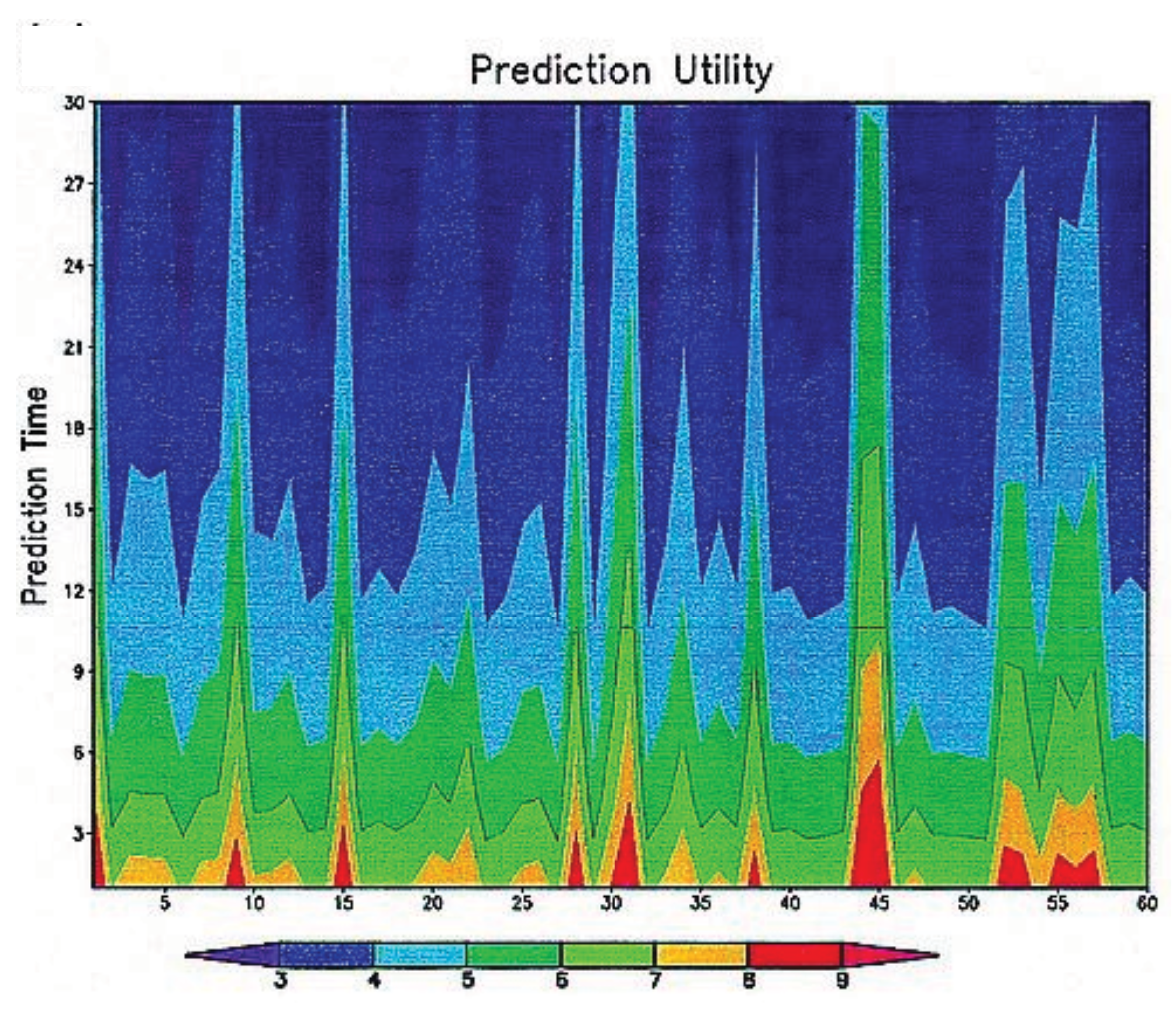
where τ is the oscillation decay time and T is the period. Asymptotically the covariance matrix of this system can be shown to be diagonal so the basis we are using is a principal component basis. Figure 2, which is reproduced from [58], shows the prediction utility of a representative sample of predictions with deterministic initial conditions with time being the vertical coordinate and sample member the horizontal coordinate. The relaxation process is evident for all predictions and one can show analytically that it is controlled by τ. Additionally it is clear that variations in prediction utility are a significant fraction of overall utility and that the character of this variation tends to persist strongly throughout any particular prediction. In other words predictions tend to have high/low utility at all times. We refer to this effect as predictability durability. Recall that the variation in utility is driven entirely in this example by the signal. Calculation of this term shows it to be
S i g n a l = x ¯ 1 σ 1 2 2 + x ¯ 2 σ 2 2 2
where the equilibrium variances are σ i 2 . Thus the signal is simply the rescaled L 2 norm squared of the prediction means (called anomalies in the climate context). In this model it appears that it takes a significant amount of time for the stochastic forcing to erode this signal which is the cause of the durability.
The simple model above was generalized in the first reference above to the time dependent case on the basis that one would expect the instability of the system to follow certain cyclic features such as the seasons. The basic qualitative results shown above however remain unaltered and in particular the variation of prediction utility was still controlled mainly by the signal even when rather large variations in the decay time τ throughout the time cycle were assumed.

5.5.2. Low Order Chaotic Systems

Such systems were originally proposed as very simple analogs for atmospheric turbulence (e.g., [68,69]). They have been extensively studied from the viewpoint of atmospheric predictability and were the original motivation for the now extensive mathematical field of chaotic dynamics. Here, unlike the previous case, there is no great separation of timescales and the growth of small perturbations occurs through non-linear interaction of the degrees of freedom rather than from random forcing from fast neglected modes. These systems are often characterized by an invariant measure that is fractal in character. This implies that the dimension of the space used to calculate probability densities is non-integral which means some care needs to be taken in defining appropriate entropic functionals. As noted earlier the non-linearity of the system but also the fractal equilibrium strange attractor mean that generally the best practical approach is Monte Carlo sampling with an appropriate coarse graining of state space. One can for example define the entropy of the equilibrium strange attractor as
E = lim M lim r 0 E ( M , r ) E ( M , r ) 1 M i = 1 M ln N i ( r ) M r d = 1 M i = 1 M ln N i ( r ) M + d ln r S ( M , r ) + d ln r
where N i ( r ) is the number of attractor sample members within a radius r of the i’th sample member; d is the so-called fractional information dimension of the attractor and M is the number of sample points. Careful comparison with (1) and (2) shows this agrees with the usual definition up to a constant which multiplies r d to give the volume element in a d dimensional space. The information dimension can be estimated by considering a sequence of decreasing r and calculating S ( M , r ) (see [70] Section 7.9). If one considers the calculation of the divergence of samples drawn from particular subregions of the attractor then a simpler expression is relevant which does not involve the information dimension:
D = lim M lim r 0 D ( M , r ) D ( M , r ) 1 M i = 1 M ln N i 1 ( r ) N i 2 ( r )
where N i 1 ( r ) is the number of the first sample members within r of the i’th first sample member while N i 2 ( r ) is the number of second sample members within the same radius of the same i’th first sample member. Naturally only a particular coarse graining D ( M , r ) is usually practically available since M is finite.
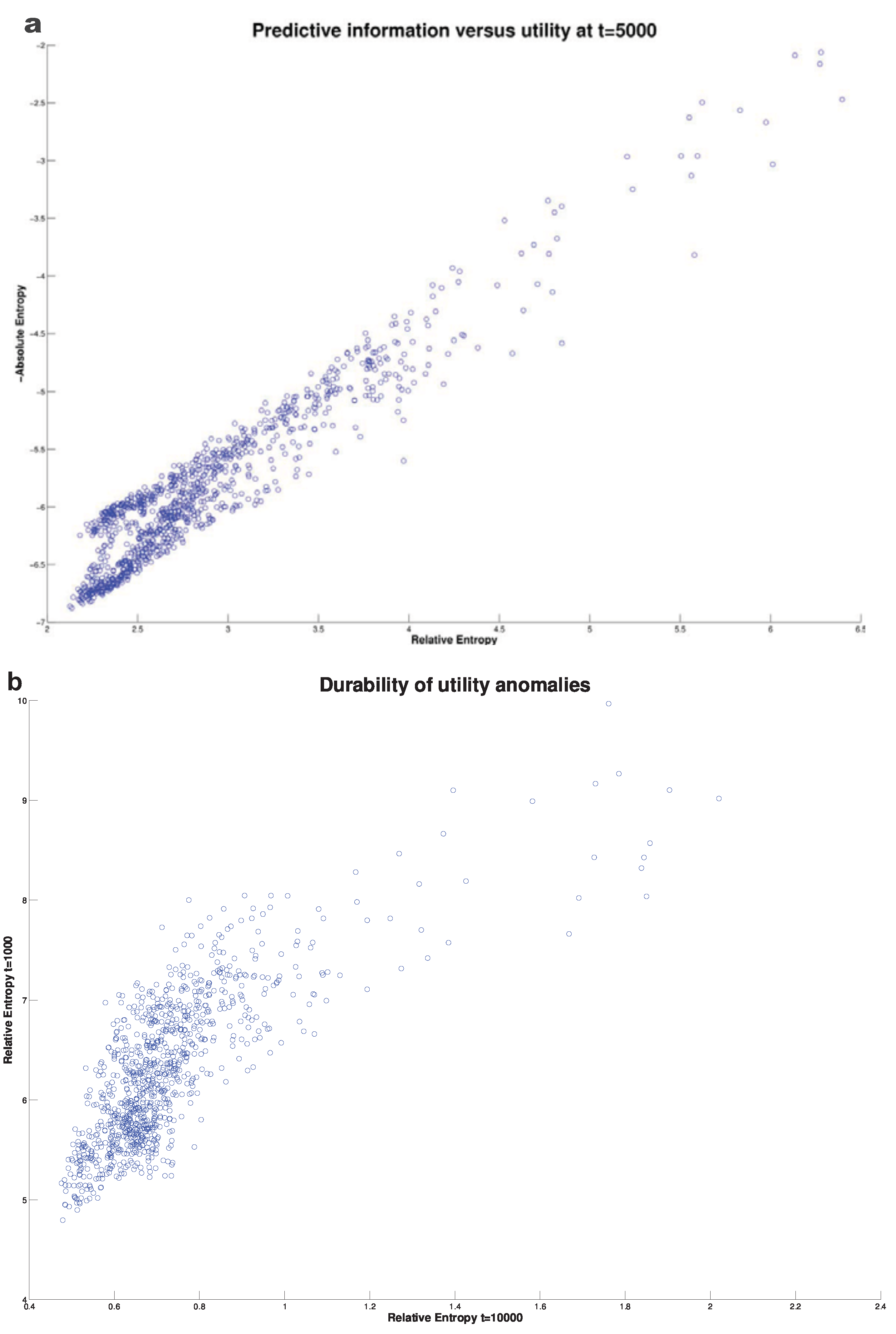
The present author (see [58]) considered the behavior of coarse grained prediction utility (23) in the classical Lorenz chaotic system [68]. Here we also compare that with the corresponding coarse grained predictive information derived from (22). A representative set of initial conditions with means drawn from equilibrium strange attractor were considered. For simplicity a (homogeneous) Gaussian distribution of two dimensions tangential to the attractor was considered with a standard deviation approximately three orders of magnitude smaller than the attractor dimensions. Thus the initial condition uncertainty was far less then the equilibrium or climatological uncertainty. The evolution of the divergence is shown in Figure 3 for a representative set of initial conditions (format is the same as Figure 2). This is reproduced from [58]. We observe again a characteristic relaxation toward equilibrium. The temporal decline in divergence is almost always monotonic although as noted in the previous subsection, this is not compulsory for the coarse grained measure used.
In stark contrast to the stochastic models considered previously, variations in the prediction utility from one set of initial conditions to another is typically strongly related to variations in predictive information. This is shown for a large sample of initial conditions in Figure 4a which shows the relationship at around halfway through the relaxation displayed in Figure 3. It is worth noting that the prediction distributions although initially chosen to be Gaussian rapidly lose this property and indeed by the time of Figure 4a it can be shown that although the variations in the predictive information correlates well with the prediction utility, variations in the Gaussian predictive information of (20) show very little correlation. This suggests that it is the higher order cumulant contributions to the entropy which are driving variations in utility. As in the stochastic case, the predictions show considerable durability. This is illustrated in Figure 4b which shows the correlation of the utility of early and late predictions.

5.5.3. Idealized Models of Turbulence

These systems attempt to simulate the realistic spectrum of turbulence with between 10 2 through 10 4 degrees of freedom and in an environment which is often homogeneous. They represent a bridge between the models of the previous subsections and realistic models of both atmosphere and ocean. The nature of the turbulence exhibited means that there is a large range of timescales present and there are large non-linear transfers of energy between modes often in the form of a scale cascade. Thus both the effects of the previous two types of models are typically present.
Calculation of information theoretic functionals for models of this dimension involves essential difficulties. As we saw in the simple chaotic model above, the most straightforward method involves a Monte Carlo method known as a prediction ensemble and some choice of coarse graining to estimate probability densities via a partitioning of state space. When we confront models with significantly higher dimensions however this problem becomes very acute since the required number of partitions increases with the power of the dimension. In order to obtain a statistically reliable estimate of density for each partition we require that the ensemble size be at least the same order as the number of partitions chosen. It is fairly clear that only approximations to the functionals will be possible in such a situation.
Two approaches have been taken to this approximation problem. The first assumes that the ensemble is sufficiently large so that low order statistical moments can be reliably calculated and then implicitly discards sample information regarding higher order moments as not known. One then uses the moment information as a hard constraint on the hypothetical distribution and derives that distribution using a maximum entropy hypothesis by deciding that no knowledge is available regarding the higher order moments. In the case that only second order or less moments are available this implies, of course, that the hypothetical distribution is Gaussian. Typically however some higher order moments can also be reliably estimated from prediction ensembles so a more general methodology is desirable. Under the appropriate circumstances, it is possible to solve for more general distributions using a convex optimization methodology. This was originally suggested by [71] and was developed extensively with the present application in mind by [72,73,74,75,76].
In the latter references moments up to order four were typically retained and so generalized skewness and kurtosis statistics were assumed to be reliably estimated from prediction ensembles. An interesting feature of these maximum entropy methods is that as more moments are retained the divergence increases (see [72]). Thus the Gaussian divergence is bounded above by that derived from the more general distributions exhibiting kurtosis and skewness effects. This is analogous with the coarse to fine graining hierarchy effect noted in the final paragraph of Section 2. One feature of many models of turbulence makes this moment maximum entropy approximation approach attractive: It is frequently observed that the low order marginal distributions are quasi Gaussian and so can usually be very well approximated by retaining only the first four moments. Such a situation contrasts strongly with that noted above in simple chaotic systems where highly non-Gaussian behavior is usual.
Another approach to the approximation issue (developed by the present author in [77]) is to accept that only marginal distributions up to a certain low order are definable from a prediction ensemble. One then calculates the average divergence with respect to all possible marginal distributions and calls the result the marginal divergence. As in the maximum entropy case, the marginal divergence of a certain order defined in this way strictly bounds from above the marginal divergences of lower order. This again is consistent with greater retention of information as higher order marginal distributions are used to discriminate between distributions. Note also that at the top of this chain sits the full divergence.
An interesting aspect of these approximations is the role of the prediction ensemble in defining either the moment constraints or the marginal distributions. Some reflection on the matter shows that in fact these objects are subject to sample error and this becomes larger as higher order approximations are considered. This suggests that in the first case the constraints assumed in deriving maximum entropy distributions should not be imposed as hard constraints but instead be weak constraints as they should reflect the presence of the sample error. This rather subtle issue has received little attention to date in the literature in the context of maximum entropy (see however [74]). See [77] for an information theoretic analysis for the simpler marginal distribution estimation case.
Four different turbulence models of varying physical complexity and dimension have been analyzed in detail using the above approximation methods:
(1)
A truncated version of Burgers equation detailed in [78]. This system is a one dimensional inviscid turbulence model with a set of conserved variables which enable a conventional Gibbs Gaussian equilibrium distribution. Predictability issues relevant to the present discussion can be found in [73,79].
(2)
The one dimensional Lorenz 1996 model of mid-latitude atmospheric turbulence detailed in [40]. This model exhibits a variety of different behaviors depending on the parameters chosen. For some settings strongly regular wave-like behavior is observed while for others a more irregular pattern occurs with some resemblance to atmospheric turbulence. The most unstable linear modes of the system tend to have most weight at a particular wavenumber which is consistent with the observed atmosphere. Predictability issues from the present perspective can be found in [73].
(3)
Two dimensional barotropic quasi-geostrophic turbulence detailed in, for example, [80]. Barotropic models refer to systems with no vertical degrees of freedom. Quasi-geostrophic models are rotating fluids which filter out fast waves (both gravity and sound) in order to focus on low frequency variability. The barotropic versions aim at simulating very low frequency variability and exclude by design variability associated with mid-latitude storms/eddies which have a typically shorter timescale. Predictability issues are discussed in [75] in the context of a global model with an inhomogeneous background state.
(4)
Baroclinic quasi-geostrophic turbulence as discussed in, for example, [81]. This system is similar to the last except simple vertical structure is incorporated which allows the fluid to draw energy from a vertical mean shear (baroclinic instability). These systems have therefore a representation of higher frequency mid-latitude storms/eddies. This latter variability is sometimes considered to be approximately a stochastic forcing of the low frequency barotropic variability although undoubtedly the turbulence spectrum is more complicated. Predictability issues from the present perspective were discussed in [82] for a model with an homogeneous background shear. They are discussed from a more conventional predictability viewpoint in [83].
Generally speaking for all systems the predictability time scale (as measured by the prediction utility) is related to the equilibration time scale of the turbulence being considered. Variations in prediction utility with initial conditions are typically similar to those seen in stochastic or simple chaotic systems. The origin of these variations is a rather complex subject and the answers obtained also vary significantly according to the system examined. In the first subsection above we considered the case where both the prediction and equilibrium distributions were Gaussian. This meant that an analytical formula involving the lowest two moments was possible and we found it convenient conceptually to separate terms into those dependent on the first and second moments of prediction distribution which we referred to as the signal and dispersion. It is important to emphasize however that this separation does not reflect a decomposition of the utility into the predictive information (the uncertainty reduction of the prediction) and a remainder term. Indeed as we saw above, the second term of Equation (21) which is included in the dispersion, is not at all related to uncertainty reduction but reflects differences in the two distributions unrelated to entropy/uncertainty or their means.
When we move to the maximum entropy approximation for prediction utility and consider moments of higher order it is possible to generalize this separation of prediction moment contributions to the divergence into those dependent on the prediction mean and those dependent on higher moments [84]. A comprehensive and rigorous description of this generalized signal/dispersion decomposition is to be found in [73]. The contribution of these two terms was examined in this reference for the first two turbulence systems listed above. The dominant contributor to overall utility variations was found to depend on the parameters chosen for the model as well as the prediction time chosen. There is also within this reference a discussion of when moments beyond the first two are important to a maximum entropy approximation retaining the first four moments.
When the higher order geostrophic turbulence models are considered (models 3 and 4 in the list above), it is usual that a considerable fraction of the equilibrium variability occurs due only to a relatively small number of modes. Predictability studies have usually focused on the equilibration behavior of such modes.
In the study of a barotropic turbulence model [75] the focus was on the first four principal components of the equilibrium distribution. The maximum entropy framework retaining four moments was used and the variability of prediction utility in terms of the generalized signal and dispersion examined with the conclusion that dispersion was overwhelmingly responsible for variations.
A baroclinic turbulence model was studied in [82]. The equilibrium turbulence spectrum in such models is well known to be dominated energetically by the large scale vertically uniform (barotropic) modes (see [25]). The predictability study therefore restricted attention to barotropic modes and the gravest four horizontal Fourier modes. The marginal distributions for both prediction and equilibrium distributions were observed to be quite close to Gaussian so only the first two moments were retained for calculation of entropic functionals by the maximum entropy method. In addition the marginal distributions with respect to these four dimensions was also calculated directly by a rather coarse partitioning. In contrast to the barotropic model above, variations in prediction utility were overwhelmingly related to variations in the (Gaussian) signal. This strong difference in predictability behavior has yet to be explained. It may be due to the importance in the latter case of the stochastic like forcing of the low frequency barotropic modes by the higher frequency baroclinic modes. These are of course absent in the barotropic turbulence case. Thus it may be that barotropic model is more like the low order chaos case while the baroclinic model is more like the simple stochastic case. This is speculation however and deeper investigation is required.

5.5.4. Realistic Global Primitive Equation Models

Such models are simplified versions of models used in real time to predict the daily weather. In contrast to most models of the previous subsection, the background for the turbulence is very inhomogeneous as it depends on geographical features such as topography and the jet stream. The latter is driven by the temperature gradient between the equator and pole and so peaks strongly in mid-latitudes. Compared with the quasi-geostrophic turbulence systems, more modes are generally required to explain the equilibrium variance: Of order around 100 compared with less than 10 for the homogeneous baroclinic quasi-geostrophic case. This dynamical situation has tended to limit the application of the approximation approaches discussed earlier. The only study conducted to date with such models from an information theoretic perspective was by the present author in [85]. This used marginal divergences on the dominant 100 equilibrium modes as well as the Gaussian maximum entropy approach discussed above. Practical prediction ensemble sizes restrict marginal divergences to order four or less. Generally speaking, marginal distributions of dynamical variables tend to be close to Gaussian however this issue remains to be systematically investigated. In the present context it was found that as initial conditions were varied, there was a correlation of order 0.8 between Gaussian estimates of divergence and those derived from marginal divergences. The latter tended to have a higher correlation among themselves.
In this system, the equilibration time scale implied by the above estimates of prediction utility is a strong inverse function of the amount of mean vertical shear present in the atmosphere. When this shear is strong as it is during winter it is between 1 and 2 months while for the summer weak shear case it is around 3 months. These estimates of predictability are significantly longer than those derived from practical weather prediction where two weeks is generally accepted to be the current predictability limit. This difference may be due to model error of practical predictions and/or due to simplifications present in the model studied in [85] which excludes important random processes such as moist convection which can provide a significant mechanism to reduce predictability.
The variation in prediction utility with respect to a representative set of initial conditions was also studied and the results found were somewhat similar to those noted in the baroclinic turbulence model discussed earlier. Overall divergence fluctuations (either Gaussian or marginal) were most strongly related to signal rather than dispersion variations. This effect was more pronounced for short range rather than long range predictions. The dispersion was however also related to utility but at a lower level than signal. Like both the stochastic and simple chaotic models discussed earlier, prediction utility variations tended to show durability i.e., high utility predictions tended to remain high throughout a prediction and vice versa.

5.5.5. Other Recent Applications

There have been interesting applications of the functionals discussed here to various climate prediction problems. This has been aided by the fact that to an even greater extent than the turbulence models discussed above, the marginal distributions observed tend to be very close to Gaussian. Indeed it is almost as if a central limit theorem operates in many complex geophysical models in such a way that many distributions of dynamical variables of interest tend to be approximately normal.
The El Nino coupled ocean/atmosphere system was considered in depth with realistic models in [86] and conclusions were broadly in line with the simple stochastic models considered earlier. In general the signal rather than dispersion played a larger role in explaining predictability variation.
The problem of global warming projection was considered from the current perspective by [87]. They used the divergence between the equilibrium distribution of various models and the present observed climate/equilibrium distribution as a measure of the veracity of a particular model. They then found a relationship between this veracity and the amplitude of projected global average warming over the next century. Models with higher veracity tended to project greater warming. In related work, global warming model errors were analyzed using an array of empirical information theoretic tools in [88]. This allowed the authors to identify global warming patterns of highest sensitivity.
Part of the issue of long term climate projection concerns its separation into that due to ocean initial conditions (natural decadal variability) and that due to changes in forcing due to the radiative effects of greenhouse gases. This issue was addressed using divergence measures of predictability in [89] where it was found that the predictability switches from the first kind to the second kind at leads of roughly 5–10 years.
The predictability of the natural decadal predictability mentioned above was analyzed in detail using divergence measures in [90]. A focus was on the behavior of the first few principal components and the authors used the Gaussian signal/dispersion decomposition to carefully analyze the nature of this predictability and the way it transfers between principal components as predictions evolve.
Finally the Gaussian signal/dispersion decomposition of divergence has been used to study the nature of the predictability of polar sea ice in a very recent unpublished study [91].

6. Conclusions and Outlook

Predictability issues in dynamical models are studied very naturally using information theoretic functionals. This follows because such variables are best considered to be random variables and entropic functionals have a very intuitive interpretation in terms of uncertainty and as measures of the differences between distributions. Adding to this attraction is the fact that these functionals exhibit invariance under general transformations of the variables describing the dynamical system and that they have deep connections with concepts from statistical physics. Indeed it is argued in this review that the utility of a prediction can be measured by the degree of statistical disequilibrium within the system. Thus the study of the predictability of a system is equivalent to the study of the nature of its statistical equilibration.
There have been several other advances in physical understanding with practical consequences which have resulted from the use of the information functionals discussed in this review:
(1)
The mechanisms responsible for variations in statistical predictability have been clarified. Traditionally it has been assumed that these are associated with variations in the instability of the initial conditions. The information theoretical analysis reveals that other mechanisms are possible. One, which has been referred to as signal here, results from variations in the “distance” with which initial conditions are from the equilibrium mean state of the system. Such excursions often take considerable time to “erode” and so are responsible for considerable practical predictability. Preliminary calculations show that this second effect may indeed be more important than the first in certain weather and climate applications. Note that this is not simply the effect of persistence of anomalies since this signal can transfer between the components of the state vector of a system. From the numerical studies conducted it appears that this second effect may be important when there is a strong separation of time scales within the system. These results are deserving of further theoretical and numerical investigation.
(2)
It has been shown that ideas from information transfer allow us to address in generality the question of improving predictions using targeted additional observations. The methods discussed above apply in the long range, non-linear regime for which previous methods are likely inapplicable.
(3)
The physical mechanism causing the decline in mid-latitude weather predictability has been studied over the full temporal range of predictions. Numerical experiments have shown the central role of vertical mean shear in controlling the equilibration/loss of predictability.
Application of the concepts considered here has often relied on the fact that the random variables under study are quasi-Gaussian since this allows application of analytical expressions. It should be emphasized however (and we saw this in Section 4) that a major attraction of information theory is the ability to go beyond this situation and consider highly non-linear and non-Gaussian distributions. As we saw in detail in Section 5, considerable progress has been made using maximum entropy methods to improve approximate calculation of functionals in high dimensional system. No doubt however more work remains in this challenging area where the curse of dimensionality always lurks.
The fundamental mechanism that drives equilibration and hence loss of predictability is the dynamical process which leads to statistical irreversibility. This, as we saw in Section 3, is intimately related to the manner in which a system is coarse grained and fundamental progress in that area will drive a deeper understanding of system predictability. Thus the expectation of the author is that further progress in the area of non-equilibrium statistical mechanics will be of great benefit to the study of the basic nature of prediction.

Acknowledgements

The author wishes to thank the Isaac Newton Institute at Cambridge University where this review was written during a visit in August 2010. Stimulating discussions over the past few years with Tim DelSole, Greg Eyink, Andy Majda, Ilya Timofeyev and Bruce Turkington are gratefully acknowledged. Support from the National Science Foundation from a variety of grants is also gratefully acknowledged.

Appendix

The proofs of the theorems in Section 3 are presented here for technical completeness.

Theorem 2

Proof. 
It follows that
( f log f ) t = f t log f + 1 = ( A f ) ( log f + 1 ) = f A ( log f + 1 ) + A ( f ) ( log f + 1 ) = f A ( log f + 1 ) + A f log f A f log f = f A + A f log f
The second term is in the form of a divergence so may be neglected after integration. We are then left with Equation (10). ☐

Theorem 3

Proof. 
The first term of Equation (12) results from Theorem 2 above. We consider therefore only the influence of the stochastic forcing part of the FPE. Let r p ln p then the FPE shows that
r t = 1 2 i j C i j p log p + 1
Now it is easy to see that
i j ( C i j u w ) = w i j ( C i j u ) + 2 ( j ( C i j u ) ) ( i w ) + C i j u i j ( w )
where we are using the symmetry of C. Using (24) with u = 1 and w = p this becomes after dropping a divergence term
r t = log p p i j D i j + 2 j D i j i p + D i j i j p
with D i j 1 2 C i j . Now it is easy to show that
log p i p = i r + i p
and so
r t = r i j D i j + 2 j D i j i r + i p log p D i j i j p
Setting u = 1 and w = r in (24) we have
i j D i j r = r i j D i j + 2 j D i j i r + D i j i j r
which enables us to write
r t = i j D i j r D i j i j r + 2 j D i j i p log p D i j i j p
The first term on the right can be dropped as before since it is of the form of a divergence. The third term can be written as
2 j D i j i p C i j i j p
which also has a divergence piece which can be dropped. We have then
r t = D i j i j r + 2 + log p i j p
Now we have
i j p log p = i log p j p log p + 1 i j p
and so
r t = D i j i log p j p i j p = p D i j i log p j log p D i j i j p = p D i j i log p j log p + i D i j j p i D i j j p
Dropping the final divergence term, using Equation (11) to drop the second term and integrating over all space we obtain the desired result (12). ☐

Theorem 4

Proof. 
Let the two processes have probability functions f and g then it follows that
( f log ( f / g ) ) t = f t log ( f / g ) + f t g t ( f / g ) = f t ( log ( f / g ) + 1 ) g t ( f / g ) = ( A f ) ( log ( f / g ) + 1 ) + ( A g ) ( f / g ) = f A A ( f ) log ( f / g ) + 1 + g A + A ( g ) ( f / g ) = A f log ( f / g ) A ( f log ( f / g ) + 1 g ( f / g ) ) = A f log ( f / g ) A ( f log ( f / g ) ) = ( A f log ( f / g ) )
In this case the entire right hand side of the evolution equation is in the form of a divergence and so may be neglected after integration is carried out. ☐

Theorem 5

Proof. 
As in the previous theorem we consider the divergence “density” function r = f log ( f / g ) . Clearly the proof of this shows we need only consider the time rate of change in this function due to C since that due to A leads to no change in time of the global integral of r. The change in r due to C is easily calculated using Equation (8):
( r c ) t = log ( f / g ) + 1 i j C i j f f g i j C i j g
where we are using the summation convention for repeated Latin indices. Writing g = f ( g / f ) and applying (24) we derive that the second term of Equation (25) is
( 2 ) = f g g f i j ( C i j f ) + 2 i ( C i j f ) i g f + C i j f i j g f
combining this with the first term we get a cancellation of the first term of ( 2 ) with part of the first term of Equation (25) and so
( r c ) t = log ( f / g ) i j C i j f 2 f g j ( C i j f ) i g f f g C i j f i j g f
Now to this equation we add and subtract the terms
2 i ( log f g ) j ( C i j f ) + C i j f i j log f g
and use Equation (24) to deduce that
( r c ) t = i j ( C i j r ) C i j f f g i j g f + i j log f g
where we are using the definition of r as well as canceling two terms involving j ( C i j f ) . It is straightforward (albeit tedious) to simplify the expression in the square brackets and obtain finally
( r c ) t = i j ( C i j r ) f C i j i ( log f g ) j ( log f g )
The first term on the right is of the form of a divergence and so as usual does not contribute to the evolution of the global integral of r C . Actually the positive definite nature of C shows that it is purely diffusive of the density r. The second term is negative almost everywhere due to the fact that C is positive definite almost everywhere and that f and g differ almost everywhere. Thus in that situation if we take the global integral of r C we conclude that the divergence declines strictly with time and satisfies the evolution Equation (13). ☐

Relationship of the Three Predictability Functionals

Label the set of statistical predictions with the initial condition vector z and drop the time variable in densities with the assumption that the prediction time outcome is described by the vector x . For a stochastic model, the prediction distribution with this initial condition vector is then
p z ( x ) = q ( x | z )
The second functional is then
P r ( z ) = q ( x | z ) log q ( x | z ) d x + h ( X ( t ) )
using the fact that all h ( X ) are equal to the equilibrium entropy for this setup. Taking expectation values with respect to the density for z which is q ( z ) we obtain
P r q = q ( z ) q ( x | z ) log q ( x | z ) d x d z + h ( X ( t ) ) = h ( X ( t ) | X ( 0 ) ) + h ( X ( t ) ) = I ( X ( t ) ; X ( 0 )
The third functional is
D ( z ) = q ( x | z ) log q ( x | z ) q ( x ) d x
since the distribution q ( x ) is always the equilibrium distribution. Again taking the same expectation value we obtain
D q = q ( z ) q ( x | z ) log q ( x | z ) q ( x ) d x d z = q ( x , z ) log q ( x , z ) q ( z ) q ( x ) d x d z = I ( X ( t ) ; X ( 0 ) )

References and Notes

  1. Sussman, G.; Wisdom, J. Chaotic evolution of the solar system. Science 1992, 257, 56. [Google Scholar] [CrossRef] [PubMed]
  2. Knopoff, L. Earthquake prediction: The scientific challenge. Proc. Nat. Acad. Sci. USA 1996, 93, 3719. [Google Scholar] [CrossRef] [PubMed]
  3. DelSole, T. Predictability and Information Theory. Part I: Measures of Predictability. J. Atmos. Sci. 2004, 61, 2425–2440. [Google Scholar] [CrossRef]
  4. Rasetti, M. Uncertainty, predictability and decidability in chaotic dynamical systems. Chaos Soliton. Fractal. 1995, 5, 133–138. [Google Scholar] [CrossRef]
  5. Jaynes, E.T. Macroscopic prediction. In Complex Systems and Operational Approaches in Neurobiology, Physics and Computers; Haken, H., Ed.; Springer: New York, NY, USA, 1985; pp. 254–269. [Google Scholar]
  6. Eyink, G.; Kim, S. A maximum entropy method for particle filtering. J. Stat. Phys. 2006, 123, 1071–1128. [Google Scholar] [CrossRef]
  7. Castronovo, E.; Harlim, J.; Majda, A. Mathematical test criteria for filtering complex systems: Plentiful observations. J. Comp. Phys. 2008, 227, 3678–3714. [Google Scholar] [CrossRef]
  8. Cover, T.; Thomas, J. Elements of Information Theory, 2nd ed.; Wiley-Interscience: New York, NY, USA, 2006. [Google Scholar]
  9. Amari, S.; Nagaoka, H. Methods of Information Geometry. Translations of Mathematical Monographs, AMS; Oxford University Press: New York, NY, USA, 2000. [Google Scholar]
  10. Risken, H. The Fokker-Planck Equation, 2nd ed.; Springer Verlag: Berlin, Germany, 1989. [Google Scholar]
  11. Daems, D.; Nicolis, G. Entropy production and phase space volume contraction. Phys. Rev. E 1999, 59, 4000–4006. [Google Scholar] [CrossRef]
  12. Garbaczewski, P. Differential entropy and dynamics of uncertainty. J. Stat. Phys. 2006, 123, 315–355. [Google Scholar] [CrossRef]
  13. Ruelle, D. Positivity of entropy production in nonequilibrium statistical mechanics. J. Stat. Phys. 1996, 85, 1–23. [Google Scholar] [CrossRef]
  14. Lebowitz, J.; Bergmann, P. Irreversible gibbsian ensembles. Ann. Phys. 1957, 1, 1–23. [Google Scholar] [CrossRef]
  15. Gardiner, C.W. Handbook of Stochastic Methods for Physics, Chemistry and the Natural Sciences. In Springer Series in Synergetics; Springer: Berlin, Germany, 2004; Volume 13. [Google Scholar]
  16. Misra, B.; Prigogine, I.; Courbage, M. From deterministic dynamics to probabilistic descriptions. Physica A 1979, 98, 1–26. [Google Scholar] [CrossRef]
  17. Goldstein, S.; Penrose, O. A nonequilibrium entropy for dynamical systems. J. Stat. Phys. 1981, 24, 325–343. [Google Scholar] [CrossRef]
  18. Courbage, M.; Nicolis, G. Markov evolution and H-theorem under finite coarse graining in conservative dynamical systems. Europhys. Lett. 1990, 11, 1. [Google Scholar] [CrossRef]
  19. Castiglione, P.; Falcioni, M.; Lesne, A.; Vulpiani, A. Chaos and Coarse Graining in Statistical Mechanics; Cambridge University Press: New York, NY, USA, 2008. [Google Scholar]
  20. van Kampen, N. Stochastic Processes in Physics and Chemistry, 3rd ed.; North Holland: Amsterdam, The Netherlands, 2007. [Google Scholar]
  21. Carnevale, G.; Frisch, U.; Salmon, R. H theorems in statistical fluid dynamics. J. Phys. A 1981, 14, 1701. [Google Scholar] [CrossRef]
  22. Carnevale, G. Statistical features of the evolution of two-dimensional turbulence. J. Fluid Mech. 1982, 122, 143–153. [Google Scholar] [CrossRef]
  23. Carnevale, G.F.; Holloway, G. Information decay and the predictability of turbulent flows. J. Fluid Mech. 1982, 116, 115–121. [Google Scholar] [CrossRef]
  24. Orszag, S. Analytical theories of turbulence. J. Fluid Mech. 1970, 41, 363–386. [Google Scholar] [CrossRef]
  25. Salmon, R. Lectures on Geophysical Fluid Dynamics; Oxford Univ. Press: New York, NY, USA, 1998. [Google Scholar]
  26. Kaneko, K. Lyapunov analysis and information flow in coupled map lattices. Physica D 1986, 23, 436. [Google Scholar] [CrossRef]
  27. Vastano, J.A.; Swinney, H.L. Information transport in spatiotemporal systems. Phys. Rev. Lett. 1988, 60, 1773. [Google Scholar] [CrossRef] [PubMed]
  28. Schreiber, T. Spatiotemporal structure in coupled map lattices: Two point correlations versus mutual information. J. Phys. 1990, A23, L393–L398. [Google Scholar]
  29. Schreiber, T. Measuring information transfer. Phys. Rev. Lett. 2000, 85, 461–464. [Google Scholar] [CrossRef] [PubMed]
  30. Liang, X.S.; Kleeman, R. Information transfer between dynamical system components. Phys. Rev. Lett. 2005, 95, 244101. [Google Scholar] [CrossRef] [PubMed]
  31. Liang, X.S.; Kleeman, R. A rigorous formalism of information transfer between dynamical system components I. Discrete maps. Physica D. 2007, 231, 1–9. [Google Scholar] [CrossRef]
  32. Liang, X.S.; Kleeman, R. A rigorous formalism of information transfer between dynamical system components II. Continuous flow. Physica D. 2007, 227, 173–182. [Google Scholar] [CrossRef]
  33. Majda, A.J.; Harlim, J. Information flow between subspaces of complex dynamical systems. Proc. Nat. Acad. Sci. USA 2007, 104, 9558–9563. [Google Scholar] [CrossRef]
  34. Zubarev, D.; Morozov, V.; Ropke, G. Statistical Mechanics of Nonequilibrium Processes. Vol. 1: Basic Concepts, Kinetic Theory; Akademie Verlag: Berlin, Germany, 1996. [Google Scholar]
  35. Palmer, T.N.; Gelaro, R.; Barkmeijer, J.; Buizza, R. Singular vectors, metrics, and adaptive observations. J. Atmos. Sci. 1998, 55, 633–653. [Google Scholar] [CrossRef]
  36. Bishop, C.; Etherton, B.; Majumdar, S. Adaptive sampling with the ensemble transform Kalman filter. Part I: Theoretical aspects. Mon. Weath. Rev. 2001, 129, 420–436. [Google Scholar] [CrossRef]
  37. Kleeman, R. Information flow in ensemble weather predictions. J. Atmos Sci. 2007, 64, 1005–1016. [Google Scholar] [CrossRef]
  38. Palmer, T. Predicting uncertainty in forecasts of weather and climate. Rep. Progr. Phys. 2000, 63, 71–116. [Google Scholar] [CrossRef]
  39. Kalnay, E. Atmospheric Modeling, Data Assimilation, and Predictability; Cambridge Univ. Press: Cambridge, UK, 2003. [Google Scholar]
  40. Lorenz, E. Predictability: A problem partly solved. In Proceedings of the Seminar on Predictability, ECMWF, Shinfield Park, Reading, England; 1996; Volume 1, pp. 1–18. [Google Scholar]
  41. Oseledec, V. A multiplicative ergodic theorem. Lyapunov characteristic numbers for dynamical systems. English transl. Trans. Moscow Math. Soc. 1968, 19, 197–221. [Google Scholar]
  42. Pesin, Y. Lyapunov characteristic exponents and ergodic properties of smooth dynamical systems with an invariant measure. Sov. Math. Dokl. 1976, 17, 196–199. [Google Scholar]
  43. Eckmann, J.; Ruelle, D. Ergodic theory of chaos and strange attractors. Rev. Mod. Phys. 1985, 57, 617–656. [Google Scholar] [CrossRef]
  44. Toth, Z.; Kalnay, E. Ensemble forecasting at NCEP and the breeding method. Mon. Weath. Rev. 1997, 125, 3297–3319. [Google Scholar] [CrossRef]
  45. Aurell, E.; Boffetta, G.; Crisanti, A.; Paladin, G.; Vulpiani, A. Growth of noninfinitesimal perturbations in turbulence. Phys. Rev. Lett. 1996, 77, 1262–1265. [Google Scholar] [CrossRef] [PubMed]
  46. Boffetta, G.; Cencini, M.; Falcioni, M.; Vulpiani, A. Predictability: A way to characterize complexity. Phys. Rep. 2002, 356, 367–474. [Google Scholar] [CrossRef]
  47. Frederiksen, J. Singular vectors, finite-time normal modes, and error growth during blocking. J. Atmos. Sci. 2000, 57, 312–333. [Google Scholar] [CrossRef]
  48. Gaspard, P.; Wang, X. Noise, chaos, and (ϵ,τ)-entropy per unit time. Phys. Rep. 1993, 235, 291–343. [Google Scholar] [CrossRef]
  49. Vannitsem, S.; Nicolis, C. Lyapunov vectors and error growth patterns in a T21L3 quasigeostrophic model. J. Atmos. Sci. 1997, 54, 347–361. [Google Scholar] [CrossRef]
  50. Houtekamer, P.L.; Lefaivre, L.; Derome, J.; Ritchie, H.; Mitchell, H.L. A system simulation approach to ensemble prediction. Mon. Weath. Rev. 1996, 124, 1225–1242. [Google Scholar] [CrossRef]
  51. Lyupanov exponents of order 10−6 − 10−7 (years)−1 have been noted in realistic model integrations which sets an analogous timescale for loss of predictability in the solar system (see [1]).
  52. Jolliffe, I.; Stephenson, D. Forecast Verification: A Practitioner’s Guide in Atmospheric Science; Wiley: Chichester, UK, 2003. [Google Scholar]
  53. Leung, L.Y.; North, G.R. Information theory and climate prediction. J. Clim. 1990, 3, 5–14. [Google Scholar] [CrossRef]
  54. It can be important in this context to be rather careful about how a (non-linear) stochastic model is formulated since results can depend on whether the Ito or Stratonovich continuum limit is assumed. A careful discussion of these issues from the viewpoint of geophysical modeling is to be found, for example, in [92].
  55. Schneider, T.; Griffies, S. A conceptual framework for predictability studies. J. Clim. 1999, 12, 3133–3155. [Google Scholar] [CrossRef]
  56. We shall refer to this functional henceforth with this terminology.
  57. We are using the conventional definition of entropy here whereas [55] use one which differs by a factor of m, the state-space dimension. Shannon’s axioms only define entropy up to an unfixed multiplicative factor. The result shown here differs therefore from those of the original paper by this factor. This is done to facilitate clarity within the context of a review.
  58. Kleeman, R. Measuring dynamical prediction utility using relative entropy. J. Atmos. Sci. 2002, 59, 2057–2072. [Google Scholar] [CrossRef]
  59. Roulston, M.S.; Smith, L.A. Evaluating probabilistic forecasts using information theory. Mon. Weath. Rev. 2002, 130, 1653–1660. [Google Scholar] [CrossRef]
  60. Bernardo, J.; Smith, A. Bayesian Theory; John Wiley and Sons: Chichester, UK, 1994. [Google Scholar]
  61. Kleeman, R.; Moore, A.M. A new method for determining the reliability of dynamical ENSO predictions. Mon. Weath. Rev. 1999, 127, 694–705. [Google Scholar] [CrossRef]
  62. Hasselmann, K. Stochastic climate models. Part I. Theory. Tellus A 1976, 28, 473–485. [Google Scholar] [CrossRef]
  63. Kleeman, R.; Power, S. Limits to predictability in a coupled ocean-atmosphere model due to atmospheric noise. Tellus A 1994, 46, 529–540. [Google Scholar] [CrossRef]
  64. Penland, C.; Sardeshmukh, P. The optimal growth of tropical sea surface temperature anomalies. J. Clim. 1995, 8, 1999–2024. [Google Scholar] [CrossRef]
  65. Kleeman, R. Spectral analysis of multi-dimensional stochastic geophysical models with an application to decadal ENSO variability. J. Atmos. Sci. 2011, 68, 13–25. [Google Scholar] [CrossRef]
  66. Saravanan, R.; McWilliams, J. Advective ocean-atmosphere interaction: An analytical stochastic model with implications for decadal variability. J. Clim. 1998, 11, 165–188. [Google Scholar] [CrossRef]
  67. DelSole, T.; Farrel, B.F. A stochastically excited linear system as a model for quasigeostrophic turbulence: Analytic results for one- and two-layer fluids. J. Atmos. Sci. 1995, 52, 2531–2547. [Google Scholar] [CrossRef]
  68. Lorenz, E.N. Deterministic non-periodic flows. J. Atmos. Sci. 1963, 20, 130–141. [Google Scholar] [CrossRef]
  69. Lorenz, E.N. Irregularity: A fundamental property of the atmosphere. Tellus A 1984, 36A, 98–110. [Google Scholar] [CrossRef]
  70. Nayfeh, A.; Balachandran, B. Applied Nonlinear Dynamics; Wiley Online Library, 1995; Volume 2, p. 685. [Google Scholar]
  71. Mead, L.R.; Papanicolaou, N. Maximum entropy in the problem of moments. J. Math. Phys. 1984, 25, 2404–2417. [Google Scholar] [CrossRef]
  72. Majda, A.J.; Kleeman, R.; Cai, D. A framework of predictability through relative entropy. Meth. Appl. Anal. 2002, 9, 425–444. [Google Scholar]
  73. Abramov, R.; Majda, A. Quantifying uncertainty for non-Gaussian ensembles in complex systems. SIAM J. Sci. Stat. Comput. 2005, 26, 411–447. [Google Scholar] [CrossRef]
  74. Haven, K.; Majda, A.; Abramov, R. Quantifying predictability through information theory: Small sample estimation in a non-Gaussian framework. J. Comp. Phys. 2005, 206, 334–362. [Google Scholar] [CrossRef]
  75. Abramov, R.; Majda, A.; Kleeman, R. Information theory and predictability for low frequency variability. J. Atmos. Sci. 2005, 62, 65–87. [Google Scholar] [CrossRef]
  76. Abramov, R. A practical computational framework for the multidimensional moment-constrained maximum entropy principle. J. Comp. Phys. 2006, 211, 198–209. [Google Scholar] [CrossRef]
  77. Kleeman, R. Statistical predictability in the atmosphere and other dynamical systems. Physica D 2007, 230, 65–71. [Google Scholar] [CrossRef]
  78. Majda, A.J.; Timofeyev, I. Statistical mechanics for truncations of the Burgers-Hopf equation: A model for intrinsic stochastic behavior with scaling. Milan J. Math. 2002, 70(1), 39–96. [Google Scholar] [CrossRef]
  79. Kleeman, R.; Majda, A.J.; Timofeyev, I. Quantifying predictability in a model with statistical features of the atmosphere. Proc. Nat. Acad. Sci. USA 2002, 99, 15291–15296. [Google Scholar] [CrossRef] [PubMed]
  80. Selten, F. An efficient description of the dynamics of barotropic flow. J. Atmos. Sci. 1995, 52, 915–936. [Google Scholar] [CrossRef]
  81. Salmon, R. Baroclinic instability and geostrophic turbulence. Geophys. Astrophys. Fluid Dyn. 1980, 15, 167–211. [Google Scholar] [CrossRef]
  82. Kleeman, R.; Majda, A.J. Predictability in a model of geostrophic turbulence. J. Atmos. Sci. 2005, 62, 2864–2879. [Google Scholar] [CrossRef]
  83. Vallis, G.K. On the predictability of quasi-geostrophic flow: The effects of beta and baroclinicity. J. Atmos. Sci. 1983, 40, 10–27. [Google Scholar] [CrossRef]
  84. Strictly speaking there are three contributions. One involves the prediction means; another the higher order prediction moments alone and thirdly a cross term involving both. The authors cited in the text group this latter term with the first and call it the generalized signal.
  85. Kleeman, R. Limits, variability and general behaviour of statistical predictability of the mid-latitude atmosphere. J. Atmos. Sci. 2008, 65, 263–275. [Google Scholar] [CrossRef]
  86. Tang, Y.; Kleeman, R.; Moore, A. Comparison of information-based measures of forecast uncertainty in ensemble ENSO prediction. J. Clim. 2008, 21, 230–247. [Google Scholar] [CrossRef]
  87. Shukla, J.; DelSole, T.; Fennessy, M.; Kinter, J.; Paolino, D. Climate model fidelity and projections of climate change. Geophys. Res. Lett. 2006, 33, L07702. [Google Scholar] [CrossRef]
  88. Majda, A.; Gershgorin, B. Quantifying uncertainty in climate change science through empirical information theory. Proc. Nat. Acad. Sci. USA 2010, 107, 14958. [Google Scholar] [CrossRef] [PubMed]
  89. Branstator, G.; Teng, H. Two limits of initial-value decadal predictability in a CGCM. J. Clim. 2010, 23, 6292–6311. [Google Scholar] [CrossRef]
  90. Teng, H.; Branstator, G. Initial-value predictability of prominent modes of North Pacific subsurface temperature in a CGCM. Clim. Dyn. 2010. [Google Scholar] [CrossRef]
  91. Bitz, C.M.; University of Washington, Seattle, WA, USA. Private communication to author, 2010.
  92. Hansen, J.; Penland, C. Efficient approximate techniques for integrating stochastic differential equations. Mon. Weath. Rev. 2006, 134, 3006–3014. [Google Scholar] [CrossRef]
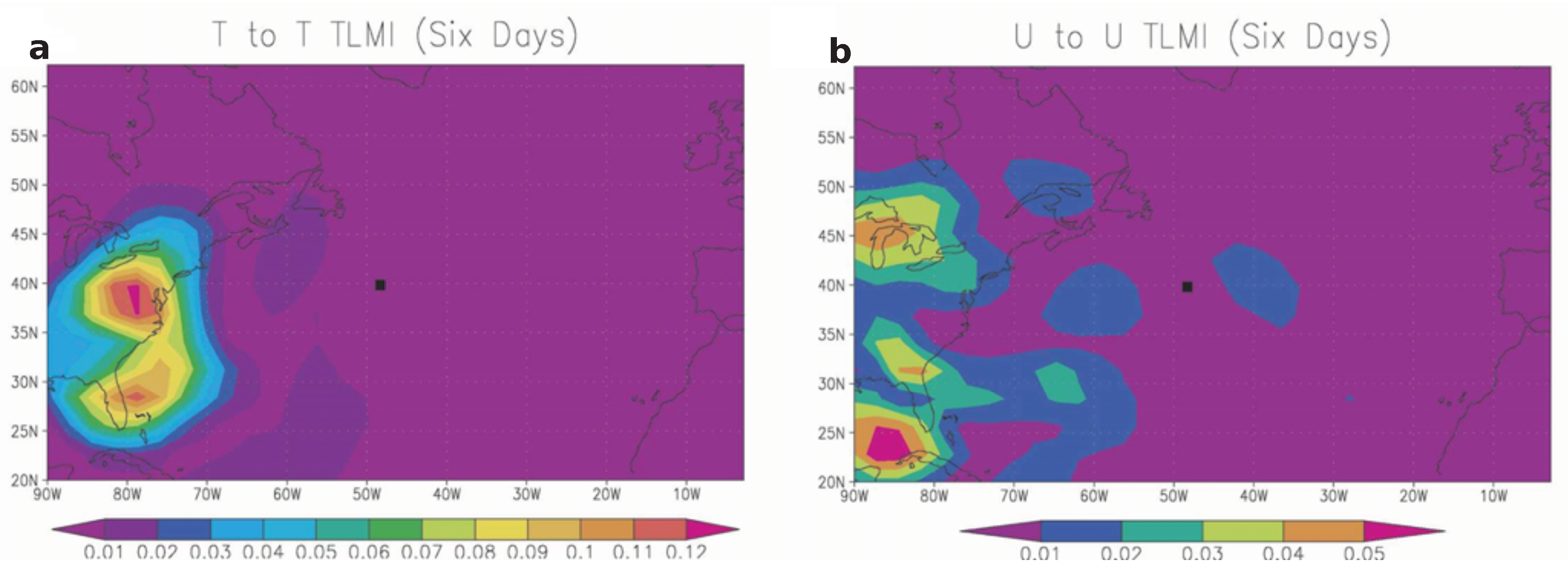
Figure 1. The TLMI regions for a six day prediction at the center of the diagram (shown as a solid circle). The left panel shows near surface temperature while the right shows zonal wind. Predictions were for the same quantities. Reproduced with permission from an original figure in Journal of the Atmospheric Sciences published by the American Meteorological Society.
Entropy 13 00612 g001
Figure 2. Prediction utility (divergence) for a series of representative initial conditions and at different prediction times. Reproduced with permission from an original figure in Journal of the Atmospheric Sciences published by the American Meteorological Society.
Entropy 13 00612 g002
Figure 3. Same as Figure 2 but for the Lorenz model. Time is expressed in number of time steps (each .001). Reproduced with permission from an original figure in Journal of the Atmospheric Sciences published by the American Meteorological Society.
Entropy 13 00612 g003
Figure 4. Top panel shows the relationship between predictive information and prediction utility at 5000 time units (see Figure 3). Bottom panel shows the relationship between utility at early (t = 1000) and late (t = 10,000) predictions.
Entropy 13 00612 g004