Entropic Regularization to Assist a Geologist in Producing a Geologic Map

Abstract

The gravity and magnetic data measured on the Earth’s surface or above it (collected from an aircraft flying at low altitude) can be used to assist in geologic mapping by estimating the spatial density and magnetization distributions, respectively, presumably confined to the interior of a horizontal slab with known depths to the top and bottom. To estimate density or magnetization distributions we assume a piecewise constant function defined on a user-specified grid of cells and invert the gravity or magnetic data by using the entropic regularization as a stabilizing function that allows estimating abrupt changes in the physical-property distribution. The entropic regularization combines the minimization of the first-order entropy measure with the maximization of the zeroth-order entropy measure of the solution vector. The aim of this approach is to detect sharp-bounded geologic units through the discontinuities in the estimated density or magnetization distributions. Tests conducted with synthetic data show that the entropic regularization can delineate discontinuous geologic units, allowing a better mapping of sharp-bounded (but buried) geologic bodies. We demonstrate the potential of the entropic regularization to assist a geologist in obtaining a geologic map by analyzing the estimated magnetization distributions from field magnetic data over a magnetic skarn in Butte Valley, Nevada, U.S.A. We show that it is an exoskarn where the ion exchange between the intrusive and the host rock occurs along a limited portion of the southern intrusive border.

1. Introduction

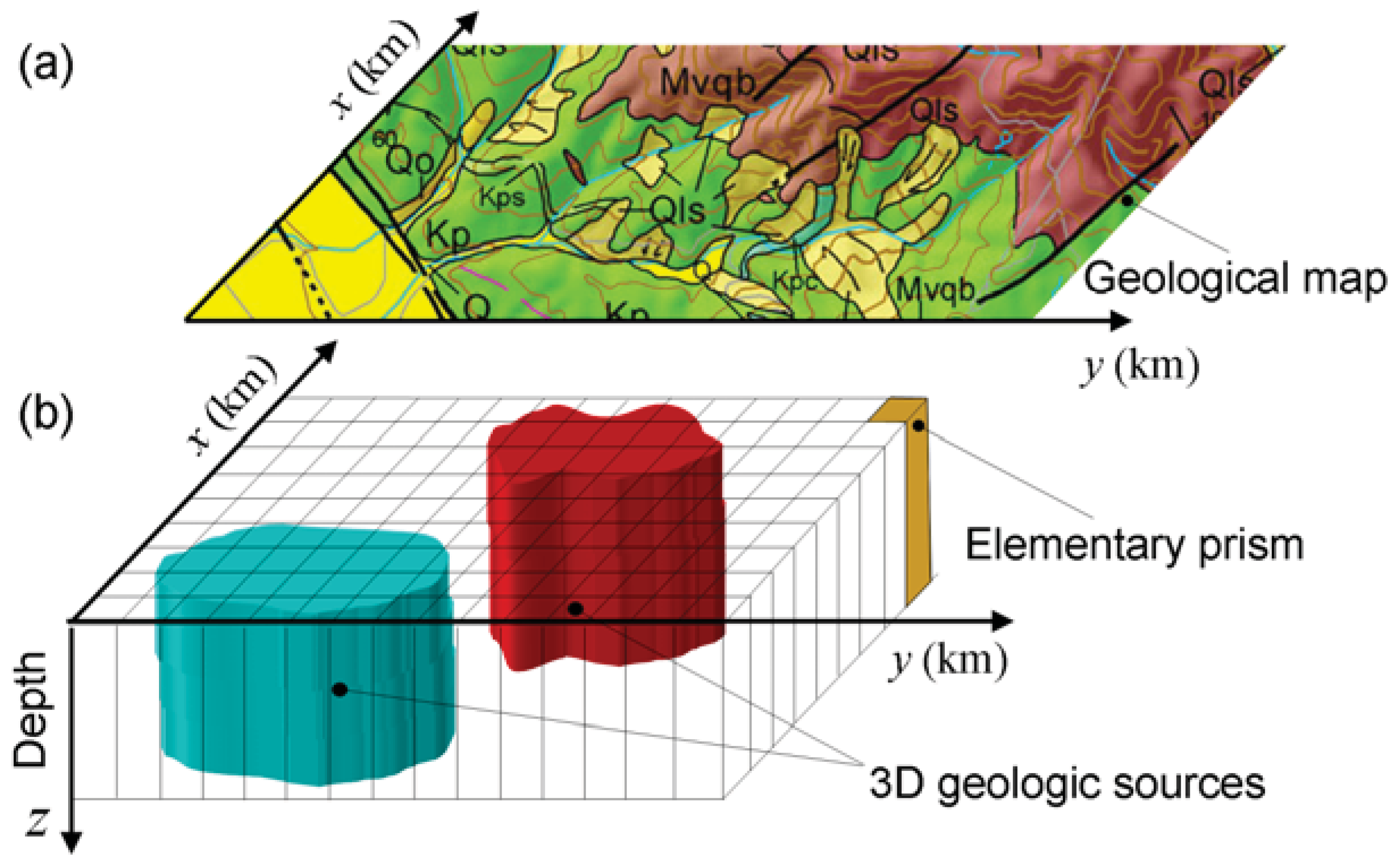
One of geologists’ objectives is to unravel the geologic history through the knowledge of the geologic processes. The evidence necessary to reconstruct the geologic history of a particular region require the production of a geologic map, which consists in identifying and demarcating geologic units. Because geologic mapping helps in understanding the geologic processes, it is used for targeting mineral resources. Hence, the first stage of mineral exploration investigation involves geologic mapping.

To produce a geologic map, geologists combine different types of information such as field, aerial and satellite data. This implies bringing together all geologic data collected mainly at the Earth’s surface to create a geologic map. Usually, the geologic interpretation of these data leads to the identification of lithology, the location of geologic contacts, faults, folds, and other geologic features. However, in the absence of outcrops one must resort to indirect measurements such as the ones provided by geophysics. Gravity and magnetic data are among the most important geophysical data used as a tool in geologic mapping [1,2,3,4,5,6] by allowing the production of magnetization and density contrast maps, respectively, thorough an inversion procedure.

Research efforts in the last decades have developed inversion methods to estimate physical-property contrast distributions (magnetization or density contrast maps) from geophysical data (gravity or magnetic data). Most of these gravity or magnetic inversion methods parameterize the Earth’s subsurface into a grid of cells distributed inside a horizontal slab with known depths to the top and bottom, and estimate the physical-property contrast of each cell element which should retrieve the geologic sources and fit the data. The inverse problem of estimating this discrete density or magnetization contrast distribution from, respectively, the gravity or the magnetic data is an ill-posed problem because its solution is unstable. The standard Tikhonov regularization method [7] is then generally used to guarantee a stable solution. Mathematically, it consists of formulating a constrained inverse problem, which is solved by the minimization of a function composed by: (1) the data-misfit function that measures a norm of the difference between the observed and predicted data, and (2) the regularizing function defined in the parameter (model) space that imposes physical or geological attributes on a solution. 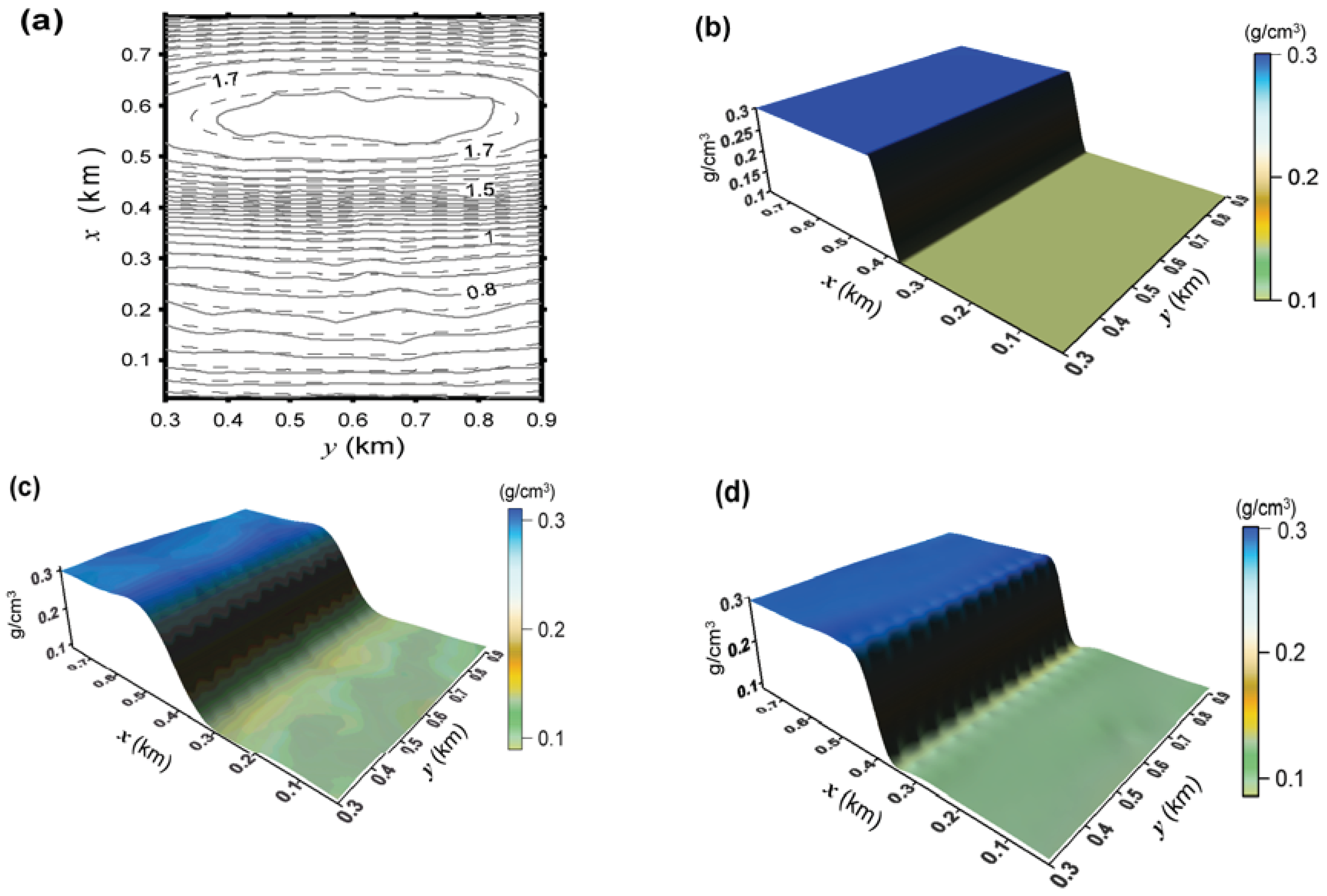In this way, the solution will be biased by the a priori information introduced by the regularizing function [8]. A classical regularizing function used in geophysics, named the first-order Tikhonov regularization, imposes a smooth character on the solution. Mathematically, it is defined as the ${\ell }_2-$norm of the first-order derivatives of the density- or magnetic-contrast distribution along two horizontal directions. In this case, the estimated physical-property distribution will be spatially smooth. This estimated smooth physical-property distribution leads to a blurred geologic map, that is, sharp geologic contacts will be displayed as smooth transitions.

To estimate nonsmooth physical-property contrast distributions through a user-specified grid of cells, we use the gravity or magnetic measurements as geophysical data and the entropic regularization as a stabilizing function that allows estimating sharp discontinuities in the physical-property contrast distribution. The entropic regularization consists in minimizing the first-order entropy measure of the vector containing the physical-property contrast distribution estimated at a discrete grid of cells and simultaneously inhibiting any excessive minimization of the zeroth-order entropy. The latter is a necessary imposition to prevent the collapse of the solution into unrealistic density or magnetic contrast distributions consisting of predominantly null values and a few unrealistically large nonnull values.

The application of the magnetization-contrast mapping, using the entropic and the first-order Tikhonov regularizations, to the magnetic anomaly over Butte Valley, NV, USA, showed an estimated source presenting one of its dimensions much larger than the other. This particular shape (which is different from the usual ring-like shape of most skarns) and the available geological information, allowed to infer that the Butte Valley anomaly is produced by an exoskarn where the ion exchange between the intrusive and the host rock occurs along a limited portion of the southern intrusive border. This example illustrates that the physical property-contrast mapping, when integrated with pertinent geological information, may effectively assist the geologist in elaborating a geological map.

2. Formulation of the Forward Problem

Consider a set of homogeneous geologic sources (geologic units) presenting physical-property distribution contrasts and horizontal tops and bottoms. The intersection of these sources with the topographic surface may be represented by a geological map Figure 1(a). We assume that depths to both the top and the bottom are known. This physical-property contrast distribution is assumed to be a piecewise constant function defined on a user-specified grid of M 3D vertical prisms juxtaposed in the x- and y-directions, which are confined in a single horizontal layer Figure 1(b). We presume that the grid encloses all geologic sources and that the tops of all prisms are at the same depth, coinciding, respectively, with the known tops of the true sources. The same is assumed for the prisms bottoms. The horizontal and vertical dimensions of each 3D prism are set by the interpreter. However, the physical property (density or magnetization intensity for a gravity or magnetic source, respectively) contrast within each prism is assumed constant but unknown and they are the parameters to be estimated from the potential-field data (gravity and magnetic data).

The discrete forward-modeling operator for the gravity and magnetic data can be expressed in matrix notation as:

d = Am

(1)

where d is an N-dimensional vector whose ith element contains the theoretical gravity or magnetic data, m is an M-dimensional vector of the prism’s physical-property contrasts (density or magnetization-intensity contrasts of a gravity or magnetic source, respectively referred to one of the sources), and $A$ is an N × M matrix of Green’s functions.

At the ith observation, the gravity and the magnetic field kernels produced by the jth prism with unitary physical-property contrast are the elements A_ij of A, which are defined by:

$$A_{ij}(r_i)=\gamma {\displaystyle {\iiint }_{V_j}\frac{z_j-z_i}{{\left|r_i-r_j\right|}^3}dv}$$

(2)

and:

$$A_{ij}(r_i)=\gamma {\displaystyle {\iiint }_{V_j}\left[L\frac{\partial }{\partial x}+M\frac{\partial }{\partial y}+N\frac{\partial }{\partial z}\right]\left[l\frac{\partial }{\partial x}+m\frac{\partial }{\partial y}+n\frac{\partial }{\partial z}\right]\frac{1}{\left|r_i-r_j\right|}dv}$$

(3)

respectively. In the above equations, $\gamma$ is Newton’s gravitational constant, $V_j$ is the volume of the jth prism, $r_i$ is the position vector of the ith gravity or magnetic observation, and $r_j$ is the position vector of the center of the jth prism. The variables $z_i$ and $z_j$ are the vertical components of the vectors $r_i$ and $r_j$, respectively. Specifically in Equation (3), $L=\cos I\cos D$, $M=\cos I\sin D$, $N=\sin I$, $l=\cos i\cos d$, $m=\cos i\sin d$, and $n=\sin i$, where $I$ is the inclination and $D$ is the azimuth of the geomagnetic field with respect to the x-axis, and $i$ is the inclination and $d$ is the azimuth of the source magnetization vector with respect to the x-axis. In the above formulation, both the geomagnetic field and the magnetization directions are assumed to be constant. The gravity or magnetic data produced by each 3D prism can be computed by the algorithm of Blakely [9].

Figure 1. Schematic representation of (a) geological map showing four geologic units (colored areas) and geologic faults (thick black lines) and (b) interpretation model consisting of a set of rectangular, 3D juxtaposed prisms. Each prism has known vertical and horizontal dimensions and horizontal top and bottom. The physical properties (density or magnetization intensity for a gravity or magnetic source, respectively) contrasts of all prisms are the parameters to be estimated from the potential-field data (gravity and magnetic data) measured over the Earth surface and produced by a set of unknown 3D geologic sources.

Figure 1. Schematic representation of (a) geological map showing four geologic units (colored areas) and geologic faults (thick black lines) and (b) interpretation model consisting of a set of rectangular, 3D juxtaposed prisms. Each prism has known vertical and horizontal dimensions and horizontal top and bottom. The physical properties (density or magnetization intensity for a gravity or magnetic source, respectively) contrasts of all prisms are the parameters to be estimated from the potential-field data (gravity and magnetic data) measured over the Earth surface and produced by a set of unknown 3D geologic sources.

3. Formulation of the Inverse Problem Using the Concept of Entropic Regularization

Let $d^o$ be a set of N observations of potential-field data (gravity or magnetic data) measured over the Earth surface and produced by a set of geologic sources. The inverse problem of estimating the associated physical-property distribution $m$ can be formulated as the minimization of the data-misfit function:

$${\varphi }^d=\frac{1}{N}\left|\right|d^o-Am|{|}_2^2$$

(4)

where $\left|\right|.|{|}_2$ is the ${\ell }_2-$norm. However, the solution of the problem of estimating the vector $\widehat{m}$ that minimizes the data-misfit function ${\varphi }^d$ [Equation (4)] is neither unique nor stable. Here, to obtain a unique and stable physical-property distribution beneath the earth from $d^o$, we employ the entropic regularization method [10,11]. Mathematically, it consists in the minimization, with respect to parameter vector $m$, of the objective function:

$$\lambda (m)={\varphi }^d+\mu {\varphi }^m(m)$$

(5)

where ${\varphi }^m(m)$ is the entropic regularization function that involves two entropy measures, and $\mu$ is a nonnegative parameter, named regularizing parameter, that controls the trade-off between the data-misfit function ${\varphi }^d(m)$ and the entropic regularization function ${\varphi }^m(m)$.

The entropic regularization function consists of two entropy measures: the zeroth-order entropy measure of $m$, given by:

$$Q_0(m)=-{\displaystyle \sum _{k=1}^M\left(\frac{m_k+\epsilon }{{\displaystyle \sum _{i=1}^M{m}_i+\epsilon }}\right)\log \left(\frac{m_k+\epsilon }{{\displaystyle \sum _{i=1}^M{m}_i+\epsilon }}\right)}$$

(6)

and the first-order entropy measure of $m$ given by:

$$Q_1(m)=-{\displaystyle \sum _{k=1}^L\left(\frac{\left|t_k\right|+\epsilon }{{\displaystyle \sum _{i=1}^L\left|t_i\right|+\epsilon }}\right)\log \left(\frac{\left|t_k\right|+\epsilon }{{\displaystyle \sum _{i=1}^L\left|t_i\right|+\epsilon }}\right)}$$

(7)

where $\epsilon$ is a small positive constant (smaller than 10⁻⁸) used to guarantee the definition of the entropy measures, L is the number of adjacent pairs of parameters, and t_k is the kth element of vector $t$ that represents the finite-difference approximation to the first derivative of $m$ along the horizontal directions.

The maximum entropy principle was first proposed as a general inference procedure by Jaynes [12,13] on the basis of Shannon’s axiomatic characterization of the amount of information [14]. Although the entropic regularization method combines the minimization of $Q_1(m)$ given in Equation (7) with the “maximization” of $Q_0(m)$ given in Equation (6) with respect to $m$, it in fact does not maximize $Q_0(m)$. Hence, the maximum entropy principle is not used to incorporate the maximum zeroth-order entropy constraint in the inverse problem by optimizing a function $Q_0(m)$. Rather, the “maximization” of $Q_0(m)$ in our case is used just to prevent its extreme minimization that occurs associated with the minimizing $Q_1(m)$.

Mathematically, the minimization of the entropy measure of order one, $Q_1(m)$, and the “maximization” of the entropy measure of order zero $Q_0(m)$ of the parameter vector $m$ can be done by minimizing the objective function $\lambda (m)$ given in Equation (5) with the entropic regularization function given by:

$${\varphi }^m(m)={\gamma }_1{Q}_1(m)-{\gamma }_0{Q}_0(m)$$

(8)

where γ₀ and γ₁ are positive numbers controlling the trade-off between the “maximization” of $Q_0(m)$ and the minimization of $Q_1(m)$. The negative sign imposed on $Q_0(m)$ in Equation (8) guarantees the “maximization” of the zeroth-order entropy measure.

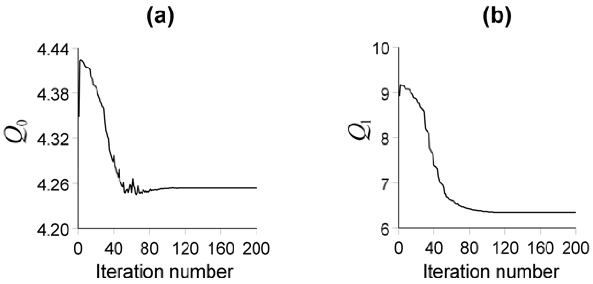
The minimizer of the nonlinear function $\lambda (m)$ given in Equation (5) is obtained iteratively by the quasi-Newton method [15,16]. We implemented the quasi-Newton method using the Broyden-Fletcher-Goldfarb-Shanno (BFGS) algorithm [16,17]. The minimization of the objective function $\lambda (m)$ [Equation (5)], with respect to the parameter vector $m$, by using the iterative quasi-Newton method, requires a stooping criterion. In our inverse problem using the entropic regularization the stopping criterion is based on the invariance of the first-order entropy function $Q_1(m)$ [Equation (7)], which, in practice, is assumed to have occurred when the following inequality holds:

$$\frac{{Q_1}^{(k-1)}(m)\text{ -}{Q_1}^{(k)}(m)}{{Q_1}^{(k-1)}(m)}\le 0.05$$

for five consecutive iterations, where ${Q_1}^{(k)}(m)$ is the value of the first-order entropy measure at the kth iteration.

The physical and geologic meaning of the entropic regularization has been explained by [17,18,19]. The minimization of the first-order entropy measure favors an estimated physical-property distribution presenting local abrupt discontinuities. However, the minimization of $Q_1(m)$ implies the minimization of $Q_0(m)$ as well, and, if the latter is not deterred, it will favor unrealistic solutions, consisting of an estimated physical-property contrast distribution with predominantly null values and a few unrealistically large nonnull values. So, the minimization of $Q_0(m)$ should be deterred. To counteract the minimization of $Q_0(m)$, it should be “maximized” not to attain in fact a maximum, but to prevent its excessive minimization. Thus, a judicious combination of the minimization of first-order entropy with maximization of zeroth-order entropy favors an estimated physical-property distribution characterized by regions with virtually constant physical property separated by sharp discontinuities.

In Equation (8) the variable γ₁ controls the number of discontinuities in the estimated physical-property distribution. An optimum value for γ₁ is the largest positive value producing no more oscillations or discontinuities than those expected for the physical-property distribution being interpreted. The variable γ₀ must be assigned the smallest value necessary to prevent an estimated physical-property distribution presenting unrealistic pattern with predominantly null values and a few unrealistically large nonnull values. Among the numerous estimated physical-property contrast distributions fitting the data with acceptable precision, the entropic regularization favors an estimated physical-property distribution with locally smooth regions separated by abrupt discontinuities.

4. Numerical Results

To evaluate the performance of the entropic regularization method, we present two tests using synthetic data. In the first one, we use gravity data produced by a simulated geologic contact. In the second test, we employ magnetic data produced by two closely spaced simulated intrusions. In these tests the gravity and the magnetic data were contaminated with pseudorandom Gaussian noise with zero mean and different standard deviations. Here, we compare the performance of the entropic regularization method with a common regularizing function used in geophysics, named first-order Tikhonov regularization, that imposes a smooth character on the solution by minimizing the ${\ell }_2-$norm of the first-order derivative of the parameters along the horizontal directions [7,20,21,22,23,24,25].

4.1. Gravity Sources

A geologic contact is the surface separating two geologic units. It is the most important feature in a geologic map and the geologic-contact mapping can benefit from the inversion of gravity data. Here, we evaluate the performance of the entropic regularization by applying it to the noise-corrupted gravity data [solid gray lines in Figure 2(a)] with a standard deviation of the pseudorandom noise of 0.01 mGal produced by a simulated geologic contact whose true theoretical density distribution is shown in Figure 2(b). The maximum data amplitude is 1.75 mGal. We simulated two adjacent geologic units (not shown) using two juxtaposed slabs with the same top depth of 0.0105 km and the same bottom depth of 0.2105 km, separated by a geologic contact. The density contrasts of these slabs with the main host rocks are 0.3 g/cm³ [blue region in Figure 2(b)] and 0.1 g/cm³ [green region in Figure 2(b)]. Hence, we simulated a geologic contact as a boundary surface between these two rocks where there is an abrupt lithological change around x = 0.4 km.

Figure 2. Test simulating a geologic contact. (a) Noise-corrupted gravity data in mGal (solid gray lines) produced by the true density-contrast distribution shown in b and fitted gravity data (dashed black lines) produced by the estimated density-contrast distribution shown in d using the entropic regularization. (b) True theoretical density-contrast distribution simulating a geologic contact. (c) Estimated density-contrast distribution produced by the first-order Tikhonov regularization. (d) Estimated density-contrast distribution produced by the entropic regularization with ${\gamma }_1$ = 1.8 and ${\gamma }_0$ = 1.2.

Figure 2. Test simulating a geologic contact. (a) Noise-corrupted gravity data in mGal (solid gray lines) produced by the true density-contrast distribution shown in b and fitted gravity data (dashed black lines) produced by the estimated density-contrast distribution shown in d using the entropic regularization. (b) True theoretical density-contrast distribution simulating a geologic contact. (c) Estimated density-contrast distribution produced by the first-order Tikhonov regularization. (d) Estimated density-contrast distribution produced by the entropic regularization with ${\gamma }_1$ = 1.8 and ${\gamma }_0$ = 1.2.

The interpretation model consists of a 16 × 24 grid of vertical prisms in the x- and y-directions, respectively, with the same horizontal dimensions of 0.05 km and tops and bottoms located at depths of 0.0105 and 0.2105 km, respectively. We impose that the top and base of the prisms coincide with the corresponding top and base of the simulated anomalous sources and presume their depths are known. The noise-corrupted gravity data were inverted using the first-order Tikhonov regularization and the entropic regularization with γ₁ = 1.8 and γ₀ = 1.2. The values assigned to γ₁ and γ₀ were obtained by trial and error. Provisionally we assign to γ₀ a small positive value, including zero, and to γ₁ a large positive value. If the solution collapses into a source whose horizontal dimensions are substantially smaller than those expected for the true source, we must increase the value assigned to γ₀. If the solution shows undefined discontinuities, we must increase γ₁. On the other hand, if the solution shows several discontinuities, we must decrease γ₁. Figure 2(c,d) shows the perspective views of the estimated density maps produced by the first-order Tikhonov regularization and by the entropic regularization, respectively.

The estimated density map produced via the first-order Tikhonov regularization [Figure 2(c)] displays the geologic contact as a smooth transition from one geological domain to another. This transition region extends 300 m along the x-direction and its presence in Figure 2(c) is inferred from the gradient changes between the x-coordinates 0.3 and 0.6 km. Consequently, the first-order Tikhonov regularization fails to map an abrupt geologic contact such as the one simulated in this test [Figure 2(b)]. On the other hand, the density map estimated by the entropic regularization [Figure 2(d)] displays steeper gradients close to the sources’ boundary, allowing a better delineation of the abrupt geologic contact whose horizontal projection is located at x = 0.4 km. Figure 2(a) shows in dashed black lines the fitted gravity data produced by the density distribution estimated through the entropic regularization [Figure 2(d)]. The corresponding anomaly using the first-order Tikhonov regularization (not shown) fits the data equally well. Figure 3 shows the absolute differences between the estimated density-contrast distribution produced by the entropic regularization [Figure 2(d)] and the estimated density-contrast distribution produced by the first-order Tikhonov regularization [Figure 2(c)]. For most of the area, this difference is about 0.0 g/cm³. Larger differences (up to ± 0.05 g/cm³) coincide with the geologic contact around x = 0.4 km.

Figure 3. Test simulating a geologic contact. Absolute differences between the estimated density-contrast distribution produced by the entropic regularization [Figure 2(d)] and the estimated density-contrast distribution produced by the first-order Tikhonov regularization [Figure 2(c)].

Figure 3. Test simulating a geologic contact. Absolute differences between the estimated density-contrast distribution produced by the entropic regularization [Figure 2(d)] and the estimated density-contrast distribution produced by the first-order Tikhonov regularization [Figure 2(c)].

4.2. Magnetic Sources

We applied the entropic regularization method to the magnetic data produced by two sources (not shown) whose adjoining vertical borders are separated by 3 km in the y-direction. Both sources have horizontal dimensions of 6 and 8 km along the x- and y-directions, respectively, and their top and base at 5 and 8 km, respectively. These sources are uniformly magnetized by induction only, in the vertical direction with intensity of 1 A/m and they simulate stocks intruded into nonmagnetic sediments or metasediments. Figure 4(a) displays in solid gray lines the simulated noise-corrupted magnetic data produced by these sources whose the maximum amplitude is 56 nT. The standard deviation of the pseudorandom noise is 0.5 nT. Figure 4(b) shows the magnetization map of these sources.

Figure 4. Test simulating two magnetic sources. (a) Noise-corrupted magnetic data in nT (solid gray lines) produced by the true magnetization-contrast distribution shown in b and fitted magnetic data (dashed black lines) produced by the estimated magnetization-contrast distribution shown in (d), using the entropic regularization. (b) True theoretical magnetization-contrast distribution simulating two magnetic sources. (c) Estimated magnetization-contrast distribution produced by the first-order Tikhonov regularization. (d) Estimated magnetization-contrast distribution produced by the entropic regularization with γ₁ = 20 and γ₀ = 3.

Figure 4. Test simulating two magnetic sources. (a) Noise-corrupted magnetic data in nT (solid gray lines) produced by the true magnetization-contrast distribution shown in b and fitted magnetic data (dashed black lines) produced by the estimated magnetization-contrast distribution shown in (d), using the entropic regularization. (b) True theoretical magnetization-contrast distribution simulating two magnetic sources. (c) Estimated magnetization-contrast distribution produced by the first-order Tikhonov regularization. (d) Estimated magnetization-contrast distribution produced by the entropic regularization with γ₁ = 20 and γ₀ = 3.

We used an interpretation model consisting of a 22 × 22 grid of vertically magnetized prisms, 1 km wide (in both x- and y-directions) with top and base at 5 and 8 km, respectively. The noise-corrupted magnetic data were inverted using the first-order Tikhonov regularization and the entropic regularization with γ₁ = 20 and γ₀ = 3. The values assigned to γ₁ and γ₀ were obtained by trial and error. Provisionally we assign to γ₀ a small positive value including zero and to γ₁ a large positive value. If the solution collapses into a source whose horizontal dimensions are substantially smaller than those expected for the true source, we must increase the value assigned to γ₀. If the solution shows undefined discontinuities, we must increase γ₁. On the other hand, if the solution shows several discontinuities, we must decrease γ₁.

Figure 4(c,d) shows the magnetization maps produced by the first-order Tikhonov regularization and by the entropic regularization, respectively. The first-order Tikhonov regularization correctly locates the sources but not their borders. The estimated magnetizations are severely smoothed, overestimated above the sources centers, and underestimated elsewhere. Moreover, the estimated magnetizations do not fall off to zero in the area between the sources, wrongly evidencing that the sources might be connected. The presence of four embryonic maxima in Figure 4(c) may also lead to the erroneous qualitative interpretation that there are four instead of two anomalous sources. Finally, there is a wide region of negative estimated magnetizations around the sources borders. On the other hand, differently from the first-order Tikhonov regularization, the entropic regularization leads to a striking improvement in correctly delineating the sources borders on the horizontal plane. Figure 4(d) shows an estimated magnetic distribution displaying steeper borders, and flat and nearly horizontal values (reflecting the source’s homogeneity) over the source. It also presents a noticeable decrease in the negative values as compared with the estimated magnetic distribution using the first-order Tikhonov regularization [Figure 4(c)]. Furthermore, the magnetization map in Figure 4(d) presents a well-defined trough between the sources allowing a better source individualization. Figure 4(a) shows the fitted anomaly (dashed black lines) produced by the magnetization distribution estimated through the entropic regularization [Figure 4(d)]. The corresponding anomaly using the first-order Tikhonov regularization (not shown) fits the data equally well.

Figure 5(a,b) shows, respectively, the behavior of functions $Q_0(m)$ and $Q_1(m)$ when minimizing $Q_1(m)$ and maximizing $Q_0(m)$.

Figure 5. Test simulating two magnetic sources. Decay of functions $Q_0(m)$(a) and $Q_1(m)$ (b) along the iterations for the solution shown in Figure 4(d).

Figure 5. Test simulating two magnetic sources. Decay of functions $Q_0(m)$(a) and $Q_1(m)$ (b) along the iterations for the solution shown in Figure 4(d).

5. Application to Real Data

Here, we discuss an interpretation of the magnetic data from Butte Valley Stock, NV, USA shown by Silva et al. [18] that compare the estimated magnetization-contrast distribution produced by the entropic regularization method with that produced by the first-order Tikhonov regularization. The Butte Valley Stock is a buried skarn located on the southern border of a nonmagnetic intrusive body emplaced in nonmagnetic sedimentary rock. A skarn is a metamorphic rock that is formed by chemical processes related mainly to an igneous environment. It usually comprises the interaction between fluids from magmatic intrusions like granites and the host carbonate-rich rocks such as limestone or dolostone. The most common form of a skarn displays a ring-like shape. In the Butte Valley Stock, prospect for porphyry copper in the 60s and 80s identified copper and gold deposits in the area. Deep drill holes indicate that the skarn has a magnetic susceptibility of 0.63 SI and lies 800 m below the flight level, overlain by nonmagnetic sediments. 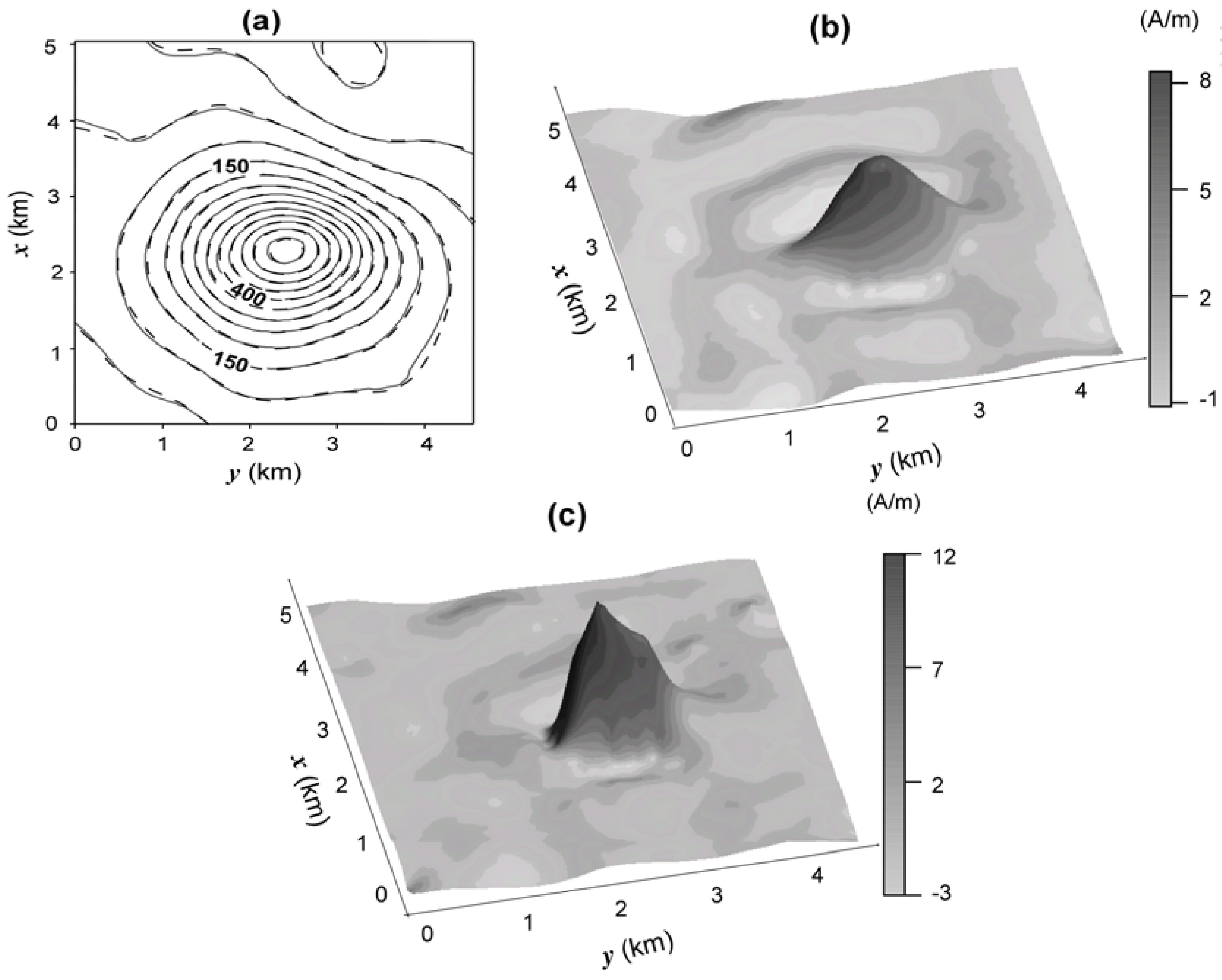Figure 6a shows the aeromagnetic total-field anomaly (gray solid lines) above Butte Valley Stock, NV, USA [5]. The flight height was 150 m above the ground surface. The geomagnetic field has inclination of 64.75° and azimuth of 15.2°. The anomaly shape suggests that the skarn magnetization is induced. Hence, the assumed inclination and the azimuth of the source magnetization vector are 64.75° and 15.2°, respectively. The interpretation model consists of a 22 × 19 grid of prisms along the x-(north-south) and y-(east-west) directions, respectively. Each prism is 0.24 km wide in both x- and y-directions, and its top and base are, respectively, 0.8 and 5 km deep.

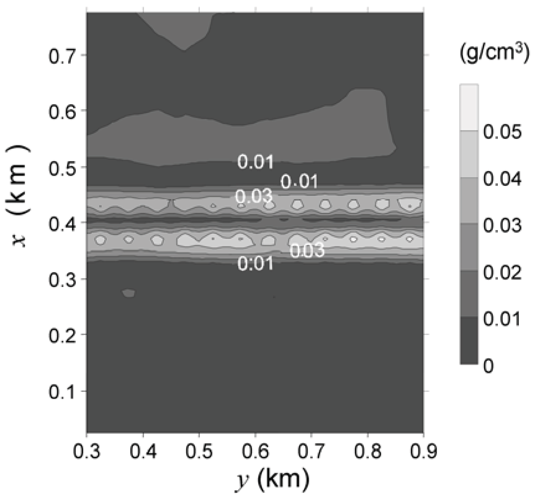
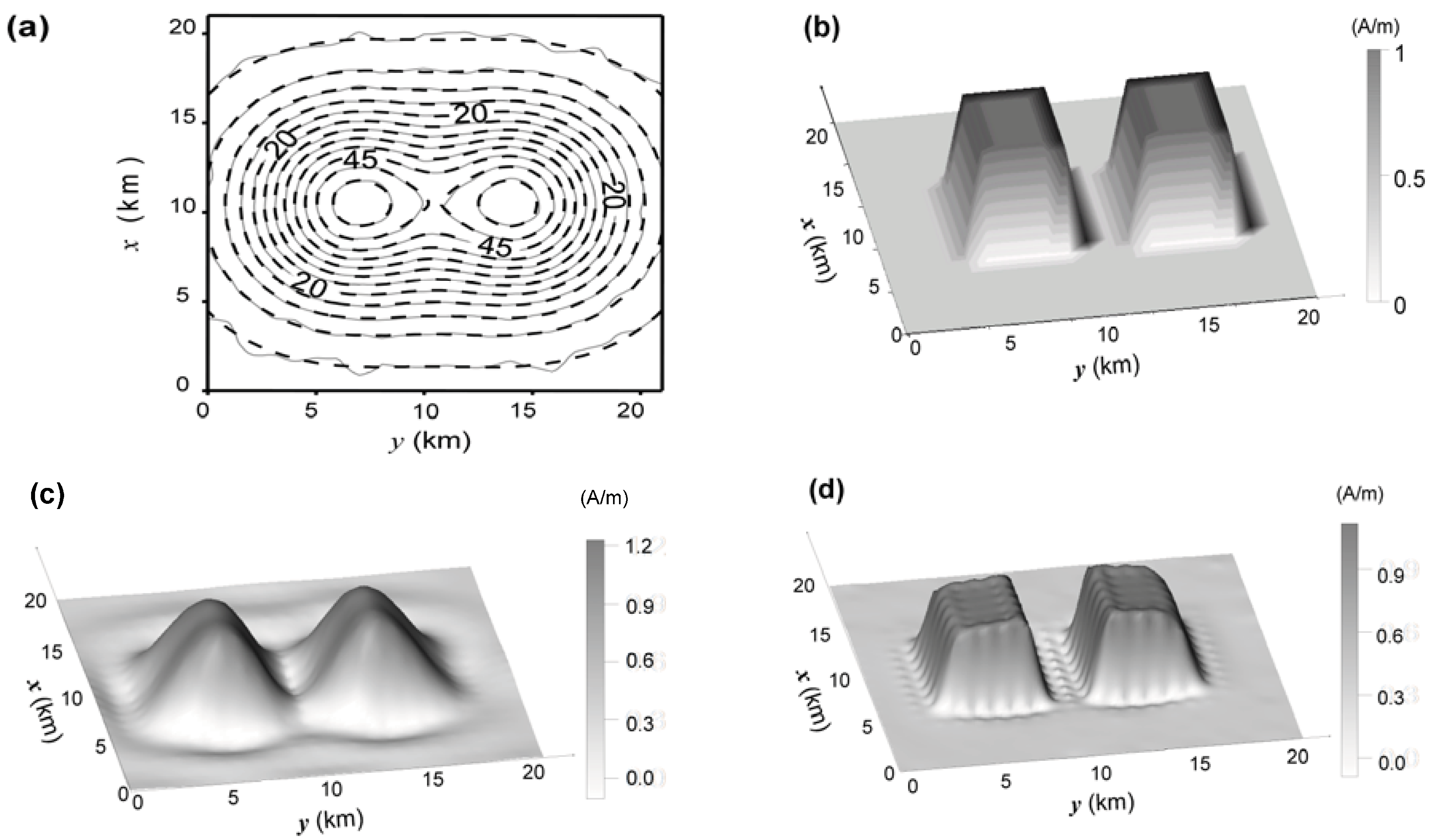
Figure 6. Butte Valley Stock. (a) Observed total-field aeromagnetic anomaly (solid gray lines) and fitted (dashed black lines) total-field anomaly (in nT) using the entropic regularization solution shown in (c). (b) Estimated magnetization-contrast distribution produced by the first-order Tikhonov regularization [18]. (c) Estimated magnetization-contrast distribution produced by the entropic regularization with γ₁ = 3,385 and γ₀ = 100 [18].

Figure 6. Butte Valley Stock. (a) Observed total-field aeromagnetic anomaly (solid gray lines) and fitted (dashed black lines) total-field anomaly (in nT) using the entropic regularization solution shown in (c). (b) Estimated magnetization-contrast distribution produced by the first-order Tikhonov regularization [18]. (c) Estimated magnetization-contrast distribution produced by the entropic regularization with γ₁ = 3,385 and γ₀ = 100 [18].

Figure 6(b,c) shows the estimated magnetization-contrast distributions using, respectively, the first-order Tikhonov regularization and the entropic regularization with γ₁ = 3,385 e γ₀ = 100. The first-order Tikhonov regularization result [Figure 6(b)] presents, as expected, a smooth transition of the estimated magnetizations from the body center to the borders, preventing a clear delineation of the source outline. Moreover, a wide region of spurious negative magnetization-contrast values shows up around the source. Conversely, the estimated magnetization-contrast distribution by the entropic regularization [Figure 6(c)] displays steeper gradients close to the source’s borders allowing a better delineation of its horizontal projection. One also notes the conspicuous reduction of the region displaying spurious negative values around the source. The entropic regularization estimates a magnetization-contrast distribution with smaller horizontal length and higher (13 A/m) maximum values of the estimated magnetization contrast. Compared with the first-order Tikhonov regularization, it produces smaller (10 A/m) maximum values of the estimated magnetization contrast. Under the hypothesis of induced magnetization, a magnetization of 13 A/m is associated with an estimated susceptibility closer to the measured value of 0.63 SI than the estimate of 10 A/m produced by the first-order Tikhonov regularization. The fitted anomaly produced by the entropic regularization is shown in Figure 6(a) in dashed black lines.

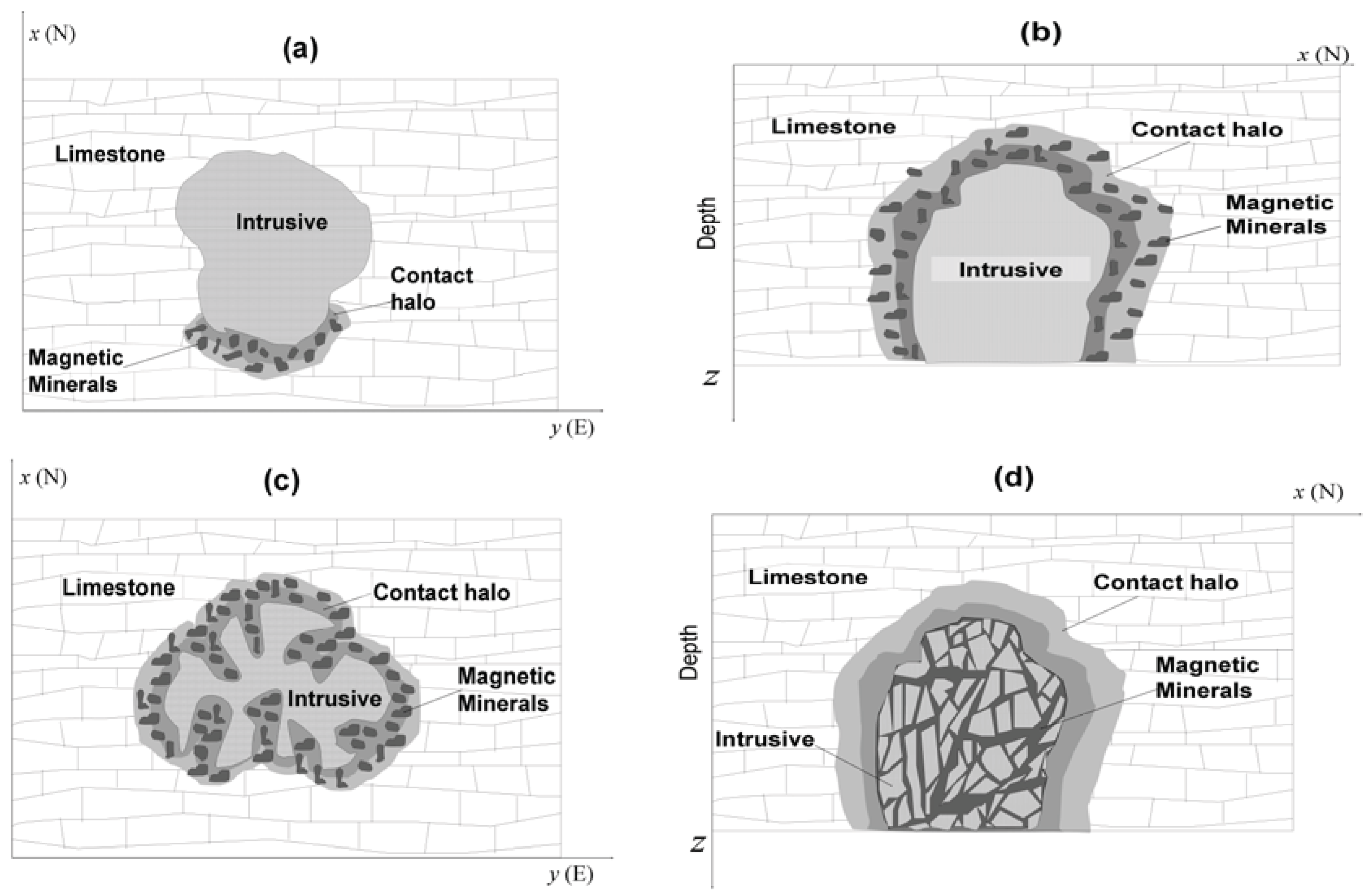
Figure 7. Butte Valley Stock. Possible skarn emplacements explaining the absence of a ring-like shape of the magnetization-contrast map. (a) Exoskarn where the ion exchange between the intrusive and the host rock occurs along a limited portion of the intrusive border. (b) Exoskarn with top located below the erosion level. (c) Exoskarn whose intrusive rock has been emplaced with an irregular shape. (d) Endoskarn where the magnetic minerals are formed along faults and joints in the intrusive rock.

Figure 7. Butte Valley Stock. Possible skarn emplacements explaining the absence of a ring-like shape of the magnetization-contrast map. (a) Exoskarn where the ion exchange between the intrusive and the host rock occurs along a limited portion of the intrusive border. (b) Exoskarn with top located below the erosion level. (c) Exoskarn whose intrusive rock has been emplaced with an irregular shape. (d) Endoskarn where the magnetic minerals are formed along faults and joints in the intrusive rock.

The most striking feature of the estimated magnetization-contrast distributions above the Butte Valley Stock [Figure 6(b,c)] is the absence of an expected ring-like shape. Neither the first-order Tikhonov regularization [Figure 6(b)] nor the entropic regularization presents noticeable difference with respect to the skarn shape. However the estimated skarn shape [Figure 6(b,c)] is in accordance with the information that the Butte Valley skarn occurs on the southern border of the intrusive as illustrated schematically in Figure 7(a). Additional explanations for the absence of a ring-like shape in the Butte Valley skarn are as follows. Firstly, the erosion level might have never exposed the intrusive top as shown in Figure 7(b). Secondly, although not very common, the intrusive might have been emplaced with an irregular shape as illustrated in Figure 7(c). Finally, the Butte Valley skarn might be an endoskarn [Figure 7(d)] instead of the more common exoskarn shown in Figure 7(a–c). In an endoskarn the magnetic minerals are formed along faults and joints inside the intrusive rock. We have discarded the hypotheses represented in Figure 7(b–d) because of: (i) the geological information that the skarn occurs at the southern portion of the intrusion, and (ii) the geophysical information derived from the magnetization-contrast map that indicates a magnetic source with one of its dimension much larger than the other. Conversely, if one of the above alternative hypotheses were true, an isometric shape for the estimated source would be expected. This example shows that a judicious combination of geological and geophysical information may produce reliable information about the sources and contribute for the elaboration of a geological map.

6. Conclusions

A geologic map is a useful tool in understanding the geologic history of an study area, which in turn is used in studying the environment of orebody emplacement to be incorporated in mine planning and scheduling. Hence, geologic mapping is of the utmost importance in locating and delineating potential mineral targets. The gravity and magnetic data measured at the earth’s surface can be used to assist in geologic mapping of the Earth’s subsurface. We have presented a method for density or magnetization mapping under the general framework of an inverse formulation. The density or magnetization map is constructed by solving a constrained inverse problem in which a regularizing function is minimized subject to fit the gravity or magnetic data, respectively. The regularizing function is the entropic regularization that combines minimization of first-order entropy with maximization of zeroth-order entropy of the estimated parameter vector which contains the magnetization or the density estimates at discrete grid of cells distributed on a horizontal slab with known depths to the top and bottom. The entropic regularization favors an estimated density- or magnetization-contrast distribution presenting locally smooth regions separated by abrupt discontinuities. When applied to the gravity or magnetic data of an area whose physical-property distribution presents sharp discontinuities produced by geologic contacts or faults, the present method has a superior performance as compared with the classical first-order Tikhonov regularization that estimates a blurred image. Numerical tests produced by simulated intrusive bodies into sedimentary rocks illustrated this advantage. Tests on field magnetic data from the skarn in Butte Valley, NV, USA, combined with available geological information indicated the source is an exoskarn where the ion exchange between the intrusive and the host rock occurs along a limited portion of the southern intrusive border, and confirm the potential of the entropic regularization in assisting a geologist to produce a geologic map.

References

1. Nabighian, M.N.; Asten, M.W. Metalliferous mining geophysics—State of the art in the last decade of the 20th century and the beginning of the new millennium. Geophysics 2002, 67, 964–978. [Google Scholar] [CrossRef]
2. Keating, P. Density mapping from gravity data using the Walsh transform. Geophysics 1992, 57, 637–642. [Google Scholar] [CrossRef]
3. Pilkington, M.; Crossley, D.J. A Kalman filter approach to susceptibility mapping. Geophysics 1987, 52, 655–664. [Google Scholar] [CrossRef]
4. Medeiros, W.E.; Silva, J.B.C. Geophysical inversion using approximate equality constraints. Geophysics 1996, 61, 1678–1688. [Google Scholar] [CrossRef]
5. Silva, J.B.C.; Hohmann, G.W. Airborne magnetic susceptibility mapping. Explor. Geophys. 1984, 15, 1–13. [Google Scholar] [CrossRef]
6. Cordell, L.; McCafferty, A.E. A terracing operator for physical property mapping with potential field data. Geophysics 1989, 54, 621–634. [Google Scholar] [CrossRef]
7. Tikhonov, A.N.; Arsenin, V.Y. Solutions of Ill-Posed Problems; V.H. Winston & Sons: Washington, DC, USA, 1977. [Google Scholar]
8. Silva, J.B.C.; Medeiros, W.E.; Barbosa, V.C.F. Potential field inversion: Choosing the appropriate technique to solve a geologic problem. Geophysics 2001, 66, 511–520. [Google Scholar] [CrossRef]
9. Blakely, R.J. Potential Theory in Gravity and Magnetic Applications; Cambridge University Press: Cambridge, MA, USA, 1995. [Google Scholar]
10. Muniz, M.B.; Ramos, F.M.; Campos Velho, H.F. Entropy- and Tikhonov-based regularization techniques applied to the backwards heat equation. Comput. Math. Appl. 2000, 40, 1071–1084. [Google Scholar] [CrossRef]
11. Ramos, F.M.; Campos Velho, H.F.; Carvalho, J.C.; Ferreira, N.J. Novel approaches on entropic regularization. Inverse Probl. 1999, 15, 1139–1148. [Google Scholar] [CrossRef]
12. Jaynes, E.T. Information theory and statistical mechanics. Phys. Rev. 1957, 106, 620–630. [Google Scholar] [CrossRef]
13. Jaynes, E.T. Information theory and statistical mechanics II. Phys. Rev. 1957, 108, 171–190. [Google Scholar] [CrossRef]
14. Shannon, C.E. The mathematical theory of communication. Bell Syst. Tech. J. 1948, 27, 379–423. [Google Scholar] [CrossRef]
15. Gill, P.E.; Murray, W.; Wright, M.H. Practical Optimization; Academic Press Inc.: London, UK, 1981. [Google Scholar]
16. Oliver, D.S.; Reynolds, A.C.; Liu, N. Inverse Theory for Petroleum Reservoir Characterization and History Matching; Cambridge University Press: Cambridge, MA, USA, 2008. [Google Scholar]
17. Silva, J.B.C.; Oliveira, F.S.; Barbosa, V.C.F.; Campos Velho, H.F. Apparent-density mapping using entropic regularization. Geophysics 2007, 72, I51–I60. [Google Scholar] [CrossRef]
18. Silva, J.B.C.; Vasconcelos, S.S.; Barbosa, V.C.F. Apparent-magnetization mapping using entropic regularization. Geophysics 2010, 75, L39–L50. [Google Scholar] [CrossRef]
19. Silva, J.B.C.; Oliveira, A.S.; Barbosa, V.C.F. Gravity inversion of 2D basement relief using entropic regularization. Geophysics 2010, 75, I29–I35. [Google Scholar] [CrossRef]
20. Barbosa, V.C.F.; Silva, J.B.C.; Medeiros, W.E. Gravity inversion of basement relief using approximate equality constraints on depths. Geophysics 1997, 62, 1745–1757. [Google Scholar] [CrossRef]
21. Barbosa, V.C.F.; Menezes, P.T.L.; Silva, J.B.C. Gravity data as a tool for detecting faults: In-depth enhancement of subtle Almada’s basement faults, Brazil. Geophysics 2007, 72, B59–B68. [Google Scholar] [CrossRef]
22. Barbosa, V.C.F.; Silva, J.B.C.; Medeiros, W.E. Practical applications of uniqueness theorems in gravimetry: Part II—Pragmatic incorporation of concrete geologic information. Geophysics 2002, 67, 795–800. [Google Scholar] [CrossRef]
23. Martins, C.M.; Barbosa, V.C.F.; Silva, J.B.C. Simultaneous 3D depth-to-basement and density-contrast estimates using gravity data and depth control at few points. Geophysics 2010, 75, I21–I28. [Google Scholar] [CrossRef]
24. Nunes, T.M.; Barbosa, V.C.F.; Silva, J.B.C. Magnetic basement depth inversion in the space domain. Pure Appl. Geophys. 2008, 165, 1891–1911. [Google Scholar] [CrossRef]
25. Silva, J.B.C.; Costa, D.C.L.; Barbosa, V.C.F. Gravity inversion of basement relief and estimation of density contrast variation with depth. Geophysics 2006, 71, J51–J58. [Google Scholar] [CrossRef]