Algorithmic Relative Complexity

Abstract

Information content and compression are tightly related concepts that can be addressed through both classical and algorithmic information theories, on the basis of Shannon entropy and Kolmogorov complexity, respectively. The definition of several entities in Kolmogorov’s framework relies upon ideas from classical information theory, and these two approaches share many common traits. In this work, we expand the relations between these two frameworks by introducing algorithmic cross-complexity and relative complexity, counterparts of the cross-entropy and relative entropy (or Kullback-Leibler divergence) found in Shannon’s framework. We define the cross-complexity of an object x with respect to another object y as the amount of computational resources needed to specify x in terms of y, and the complexity of x related to y as the compression power which is lost when adopting such a description for x, compared to the shortest representation of x. Properties of analogous quantities in classical information theory hold for these new concepts. As these notions are incomputable, a suitable approximation based upon data compression is derived to enable the application to real data, yielding a divergence measure applicable to any pair of strings. Example applications are outlined, involving authorship attribution and satellite image classification, as well as a comparison to similar established techniques.

1. Introduction

Both classical and algorithmic information theory aim at quantifying the information contained within an object. Classical Shannon’s information theory [1] has a probabilistic approach. As it is based on the uncertainty of the outcomes of random variables, it cannot describe the information content of an isolated object, if no a priori knowledge is available. The primary concept of algorithmic information theory is instead the information content of an individual object, which is a measure of how difficult it is to specify how to construct or calculate that object. This notion is also known as Kolmogorov complexity [2]. This area of study allowed formal definitions of concepts which were previously vague, such as randomness, Occam’s razor, simplicity and complexity. The theoretical frameworks of classical and algorithmic information theory are similar, and many concepts exist in both, sharing various properties (a detailed overview is to be found in [2]).

In this paper we introduce the concepts of cross-complexity and relative complexity, the algorithmic versions of cross-entropy and relative entropy (also known as Kullback-Leibler divergence). These are defined between any two strings x and y respectively as the computational resources needed to specify x only in terms of y, and the compression power which is lost when using such a representation for x instead of its most compact one, which has length equal to its Kolmogorov complexity.

As the introduced concepts are incomputable, we rely on previous work which approximates the complexity of an object with the size of its compressed version, so as to quantify the shared information between two objects [3]. We derive a similarity measure from the concept of relative complexity that can be applied between any two strings.

Previously, a correspondence between relative entropy and compression-based similarity measures was considered in [4] for static encoders, directly related to the probability distributions of random variables. Additionally, methods to compute the relative entropy between any two strings have been proposed by Ziv and Merham [5] and Benedetto et al. [6]. The concept of relative complexity introduced in this work may be regarded as an expansion of [4], and experiments on authorship attribution contained in [6] are repeated in this paper using the proposed distance with better results.

This paper is organized as follows. We recall basic concepts of Shannon entropy and Kolmogorov complexity in Section 2, focusing on their shared properties and their relation with data compression. Section 3 introduces the algorithmic cross-complexity and relative complexity, while in Section 4 we define their computable approximations using compression-based techniques. Practical applications and comparisons with similar methods are reported in Section 5. We conclude in Section 6.

2. Preliminaries

2.1. Shannon Entropy and Kolmogorov Complexity

The Shannon entropy in classical information theory [1] is an ensemble concept; it is a measure of the degree of ignorance about the outcomes of a random variable X with a given a priori probability distribution p(x) = P(X = x):

$$H(X)=-{\displaystyle \sum _{x}p(x)\log (p(x))}$$

(1)

This definition can be interpreted as the average length in bits needed to encode the outcomes of X, which can be obtained, for example, through the Shannon-Fano code, to achieve compression. An approach of this nature, with probabilistic assumptions, does not provide the informational content of individual objects and their possible regularity. Instead, the Kolmogorov complexity K(x), or algorithmic complexity, evaluates an intrinsic complexity for any isolated string x, independently of any description formalism. In this work we consider the “prefix” algorithmic complexity of a binary string x, which is the size in bits (binary digits) of the shortest self-delimiting program q used as input by a universal Turing machine to compute x and halt:

$$K(x)=\underset{q\in Qx}{\min }\left|q\right|$$

(2)

with Qx being the set of instantaneous codes that generate x. One interpretation of K(x) is the quantity of information needed to recover x from scratch. The original formulation of this concept is independently due to Solomonoff [7], Kolmogorov [8], and Chaitin [9]. Strings exhibiting recurring patterns have low complexity, whereas the complexity of random strings is high and almost equals their own length. It is important to remark that K(x) is not a computable function of x. A formal link between entropy and algorithmic complexity has been established in the following theorem [2].

Theorem 1: The sum of the expected Kolmogorov complexities of all the code words x which are output of a random source X, weighted by their probabilities p(x), equals the statistical Shannon entropy H(X) of X, up to an additive constant. The following holds, if the set of outcomes of X is finite and each probability p(x) is computable:

$$H(X)\le {\displaystyle \sum _{x}p(x)K(x)\le H(X)+K(p)+O(1)}$$

(3)

where K(p) represents the complexity of the probability function itself. So for simple distributions the expected complexity approaches the entropy.

2.2. Mutual Information and Other Correspondences

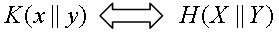
The conditional complexity K(x|y) of x related to y quantifies the information needed to recover x if y is given as an auxiliary input to the computation. Note that if y carries information which is shared with x, K(x|y) will be considerably smaller than K(x). In the other case, if y gives no information at all about x, then K(x|y) = K(x) + O(1), and K(x,y) = K(x) + K(y), with the joint complexity K(x,y) being defined as the length of the shortest program which outputs x followed by y. For all these definitions, the desirable properties of analogous quantities in classical information theory related to random variables, i.e., the conditional entropy H(X|Y) of X given Y and the joint entropy of X and Y H(X,Y), hold [2].

An important issue of the information content analysis is the estimation of the amount of information shared by two objects. From Shannon’s probabilistic point of view, it occurs via the mutual information I(X,Y) between two random variables X and Y, defined in terms of entropy as:

$$I(X,Y)=H(X)-H(X|Y)=H(X)+H(Y)-H(X,Y)$$

(4)

It is possible to obtain a similar estimation of shared information in the Kolmogorov complexity framework by defining the algorithmic mutual information between two strings x and y as:

$$I(x:y)=K(x)-K(x|y)=K(x)+K(y)-K(x,y)$$

(5)

valid up to an additive term $O(\log |xy|)$. This definition resembles (4) both in properties and nomenclature [2]: one important shared property is that if $I(x:y)=0$, then

K(x,y) = K(x) + K(y) + O(1)

(6)

and x and y are, by definition, algorithmically independent.

What probably is the greatest success of these concepts is enabling the ultimate estimation of shared information between two objects: the Normalized Information Distance (NID) [3]. The NID is a similarity metric minimizing any admissible metric, proportional to the length of the shortest program that computes x given y, as well as computing y given x. The distance computed on the basis of these considerations is, after normalization:

$$NID(x,y)=\frac{\max \{K(y|x),K(x|y)\}}{\max \{K(x),K(y)\}}=\frac{K(x,y)-\min \{K(x),K(y)\}}{\max \{K(x),K(y)\}}+O(1)$$

(7)

where, in the right term of the equation, the relation between conditional and joint complexities $K(x|y)=K(x,y)-K(y)+O(1)$ is used to substitute the terms in the dividend. The NID is a metric, so its result is a positive quantity r in the domain 0 $\le$ r $\le$ 1, with r = 0 iff the objects are identical and r = 1 representing maximum distance between them.

The value of this similarity measure between two strings x and y is directly related to the algorithmic mutual information, with $NID(x,y)+\frac{I(x:y)}{\max \{K(x),K(y)\}}=1.$ This can be shown, assuming the case $K(x)\le K(y)$ with the case $K(x)>K(y)$ being symmetric and up to an additive constant O(1), as follows: $\frac{K(x,y)-K(x)}{K(y)}+\frac{K(x)+K(y)-K(x,y)}{K(y)}=1$.

Another Shannon-Kolmogorov correspondence is the one between rate-distortion theory [1] and Kolmogorov structure functions [10], which aim at separating the meaningful (structural) information contained in an object from its random part (its randomness deficiency), characterized by less meaningful details and noise.

2.3. Compression-Based Approximations

As the complexity K(x) is not a computable function of x, a suitable approximation is defined by Li and Vitányi by considering it as the size of the ultimate compressed version of x, and a lower bound for what a real compressor can achieve. This allows approximating K(x) with C(x) = K(x) + k, i.e., the length of the compressed version of x obtained with any off-the-shelf lossless compressor C, plus an unknown constant k: the presence of k is required by the fact that it is not possible to estimate how close to the lower bound represented by K(x) this approximation is. The conditional complexity K(x|y) can be also estimated through compression [11] while the joint complexity K(x,y) is approximated by compressing the concatenation of x and y. Equation (7) can then be estimated through the Normalized Compression Distance (NCD) as follows:

$$NCD(x,y)=\frac{C(x,y)-\min \{C(x),C(y)\}}{\max \{C(x),C(y)\}}$$

(8)

where C(x,y) represents the size of the file obtained by compressing the concatenation of x and y . The NCD can be explicitly computed between any two strings or files x and y and it represents how different they are. The conditions for NCD to be a metric hold under certain assumptions [12]: in practice the NCD is a non-negative number 0 ≤ NCD ≤ 1 + e, with the e in the upper bound due to imperfections in the compression algorithms, usually assuming a value below 0.1 for most standard compressors [4]. The NCD has a characteristic data-driven, parameter-free approach that allows performing clustering, classification and anomaly detection on diverse data types [12,13].

3. Cross-Complexity and Relative Complexity

3.1. Cross-Entropy and Cross-Complexity

Let us start by recalling the definition of cross-entropy in Shannon’s framework:

$$H(X\oplus Y)=-{\displaystyle \sum _i{p}_X(i)\log p_Y(i)}$$

(9)

with $p_X(i)=p(X=i)$ and $p_Y(i)=p(Y=i)$. The cross-entropy represents the expected number of bits needed to encode the outcomes of a variable X as if they were outcomes of another variable Y. Therefore, the set of outcomes of X is a subset of the outcomes of Y. This notion can be brought in the algorithmic framework to determine how to measure the computational resources needed to specify an object x in terms of another one y.

We introduce the cross-complexity $K(x\oplus y)$ of x given y as the shortest program which outputs x by reusing instructions from the shortest program generating y, as follows. Consider two binary strings x and y, and assume to have available an optimal code $y*$ which outputs y, such that |$y*$|=K(y). Let S be the set of all possible binary substrings of $y*$, with $\left|S\right|=(|y*|+1)|y*|/2$. We use an oracle to determine which elements of S are self-delimiting programs which halt when fed to a reference universal prefix Turing Machine U [14], so that U halts with such a segment of $y*$ as input. Let the set of these halting programs be Y, and let the set of outputs of Y be Z, with $Z=\{U(u):u\in Y\}$, with $U^{-1}(U(u))=u$. If two different segments $u_1$ and $u_2$ give as output the same element of Z, i.e., $U(u_1)=U(u_2)$, then if $\left|u_1\right|<\left|u_2\right|$, or if $\left|u_1\right|=\left|u_2\right|$ and $u_1$ comes before $u_2$ in standard enumeration, $U^{-1}(U(u_2))=U^{-1}(U(u_1))=u_1$. Finally, determine an integer n and the way to divide x in n subwords $x=x_1{x}_2\mathrm{..}{x}_i\mathrm{..}{x}_n$, so that the sum $n+{\displaystyle \sum _{j=1,x_j\in Z}^n|U^{-1}(x_j)|+{\displaystyle \sum _{h=1,x_h\notin Z}^n|sd(x_h)|}}$ is minimal, where $sd(x_i)$ is the plain self-delimiting version of the string $x_i$, with $|sd(x_i)|=\left|x_i\right|+O(\log |x_i|)$. This way we can write x as a binary string preceded by a self-delimiting program of constant length c telling U how to interpret the next commands, followed by 1$U^{-1}(x_i)$ for the ith segment $x_i$ of x = $x_1{x}_2\mathrm{...}{x}_n$ if $x_i$ is replaced by $U^{-1}(x_i)\in Y$ and by 0 $sd(x_i)$ if this segment $x_i$ is replaced by its self-delimiting version $sd(x_i)$.

This way, x is coded into some concatenation of subsegments of $y*$ expanding into segments of x, prefixed with 1, and the remaining segments of x in self-delimiting form prefixed with 0. The above sum is prefixed by a c-bit program (self-delimiting), which depends on the Turing Machine adopted, that tells U how to compute x from the following commands. The total forms the code $(x\oplus y)*$, with $|(x\oplus y)*|=K(x\oplus y)$.

The reference universal Turing machine U on input $sd(x)y*$, prefixed by an appropriate program, enumerates at first the sets S, Y, and Z. On their basis, U builds the code $(x\oplus y)*$, and finally halts if both x and y are finite. Moreover, U with $(x\oplus y)*$ as input computes as output x and halts.Note that by definition of cross-complexity:

$$K(x\oplus y)\le \left|x\right|+O(\log |x|)$$

(10)

$$K(x)\le K(x\oplus y)+O(1)$$

(11)

$$K(x\oplus x)=K(x)+O(1)$$

(12)

So, $K(x\oplus y)$ is lower bounded by the plain Kolmogorov complexity K(x) of x (10), and reaches its upper bound if the sum ${\displaystyle \sum _{j=1,x_j\in Z}^n|U^{-1}(x_j)|}$, as in the above definition, is equal to 0 (11). For the case x=y, constructing the code $(x\oplus x)*$ implies reusing the shortest code x* of length K(x) which outputs x, hence (12). The cross-complexity $K(x\oplus y)$ is different from the conditional complexity $K(x|y)$: in the former x is expressed in terms of a description tailored for y, whereas in the latter the object y is an auxiliary input that is given “for free” and does not count in the estimation of the computational resources needed to specify x.

Key cross-entropy’s properties hold for this definition of algorithmic cross-complexity:

• The cross-entropy $H(X\oplus Y)$ is lower bounded by the entropy $H(X)$, i.e., $H(X\oplus Y)\ge H(X)$, as the cross-complexity in (11).
• The identity $\begin{array}{cc}H(X\oplus Y)=H(X),& if\end{array}X=Y$ also holds up to an additive term (12). Note that the strongest $\begin{array}{cc}H(X\oplus Y)=H(X),& iff\end{array}X=Y$, does not hold in the algorithmic framework. Consider the case of x being a substring of y, with y* containing the shortest code x* to output x, then $K(x\oplus y)$ = $K(x)$ + O(1).
• The cross-entropy $H(X\oplus Y)$ of X given Y and the entropy H(X) of X share the same upper bound log(N), where N is the number of possible outcomes of X, as algorithmic complexity and algorithmic cross-complexity. This property follows from the definition of algorithmic complexity and (10).

3.2. Relative Entropy and Relative Complexity

The definition of algorithmic relative complexity derives from the idea of relative entropy (or Kullback-Leibler divergence) related to two probability distributions X and Y. This divergence represents the expected difference in the number of bits required to code an outcome i of X when using an encoding based on Y, instead of X [15]:

$$D(X||Y)={\displaystyle \sum _i{P}_X(i)\log \frac{P_X(i)}{P_Y(i)}}$$

(13)

with $D(X||Y)\ge 0,$ equality $\begin{array}{cc}iff& X=Y\end{array}$, and $D(X||Y)\ne D(Y||X)$. $D(X||Y)$ is not a metric, as it is not symmetric and the triangle inequality does not hold [16]. What is more meaningful for our purposes is the definition of relative entropy expressed in terms of difference between cross-entropy and entropy:

$$D(X||Y)=H(X\oplus Y)-H(X)$$

(14)

We define the relative complexity in terms of cross-entropy according to (14), replacing entropies by complexities. For two finite binary strings x and y the algorithmic relative complexity $K(x||y)$of x towards y is equal to the difference between the cross-complexity $K(x\oplus y)$ and the Kolmogorov complexity K(x):

$$K(x||y)=K(x\oplus y)-K(x)$$

(15)

The relative complexity between x and y represents the compression power lost when compressing x by describing it only in terms of y, instead of using its most compact representation. We may also regard $K(x||y)$, as for its counterpart in Shannon framework, as a quantification of the distance between x and y. It is desirable that the key properties of (13) hold also for (15). As in (13), the algorithmic relative complexity $K(x||y)$ of x given y is positively defined: $0\le K(x||y)\le \left|x\right|+O(\log |x|)$, $\forall x,y$, as a consequence of (10) and (12).

4. Computable Approximations

4.1. Computable Algorithmic Cross-Complexity

The incomputability of algorithmic cross-complexity and relative complexity is a direct consequence of the incomputability of their Kolmogorov complexity components. We once again rely on data compression to approximate the relative complexity $K(x\oplus y)$ through $C(x\oplus y)$, following the ideas contained in [12]. To encode a string x according to the description of another string y, one could first compress y and then use the patterns found in y to compress x. But with such an approach, it would be difficult to compare the cross-compression of x given y to the compression factor of x obtained through a standard compression algorithm. Consider compressors of the Lempel-Ziv family, which use dynamic dictionaries built on the fly as a string x is analyzed: it would not be fair to compare the compression of x achieved through such a dictionary to the cross-compression obtained by compressing x with the full, static dictionary extracted by y. To reach our goal we want instead to simulate the behaviour of a real compressor which processes in parallel x and y, exploiting on the fly the information and redundancies contained in y to compress x. Such cross-compressor would keep relative entropy’s key idea of encoding the outcomes of a variable X using a code which is optimal for another random variable Y, and is implemented as follows.

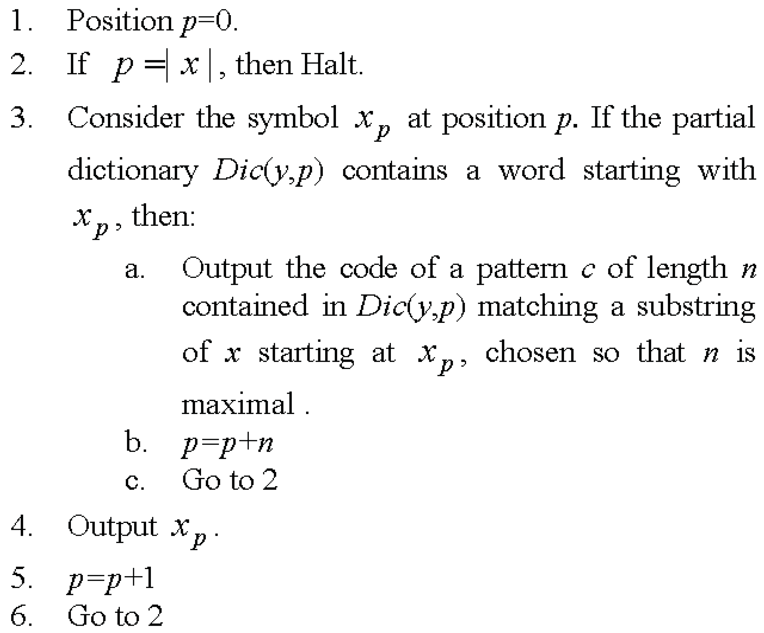
Consider two strings x and y, with $\left|y\right|=n$. Suppose to have n available dictionaries Dic(y,i), with $i=\mathrm{0...}n$, extracted from n substrings $z_i$ of y of length i, so that $z_i=y_0{y}_1\mathrm{..}{y}_i$. A representation $C(x\oplus y)*$ of x, of initial length |x|, is then computed as in the pseudo-code listed in Figure 1. Its length $C(x\oplus y)$ represents then the size of x compressed by the dictionary generated from y, if a parallel processing of x and y is simulated.

It is possible to create a unique dictionary for a string y as a hash table containing couples (key, value), where key is the position of y in which the pattern occurs the first time, and value contains the full pattern. Then $C(x\oplus y)*$ can be computed by matching the patterns in x with the portions of the dictionary of y with key < p, where p is the actual position in x. So, for two strings x and y with $\left|x\right|<\left|y\right|$, only the first |x| elements of y will be considered.

Figure 1. Pseudo-code to generate an approximation $C(x\oplus y)$ of the cross-complexity $K(x\oplus y)$ between two strings x and y.

Figure 1. Pseudo-code to generate an approximation $C(x\oplus y)$ of the cross-complexity $K(x\oplus y)$ between two strings x and y.

We report in Table 1 and Table 2 a practical example. Consider two ASCII-coded strings A = {abcabcabcabc} and B = {abababababab}. By applying the LZW algorithm, we extract and use two dictionaries Dict(A) and Dict(B) to compress A and B into two strings $A*$ and $B*$ of length C(A) and C(B), respectively. By applying the pseudo-code in Figure 1 we compute $(A\oplus B)*$ and $(B\oplus A)*$, of lengths $C(A\oplus B)$ and $C(B\oplus A)$.

Table 1. An example of cross-compression. Extracted dictionaries and compressed versions of A and B, plus cross-compressions between A and B, computed with the algorithm reported in Figure 1.

A	$Dict(A)$	$A*$	$(A\oplus B)*$	B	$Dict(B)$	$B*$	$(B\oplus A)*$
a				a
b	ab = <256>	a	a	b	ab = <256>	A	a
c	bc = <257>	b	b	a	ba = <257>	B	b
a	ca = <258>	c	c	b
b				a	aba = <258>	<256>	<256>
c	abc = <259>	<256>	<256>	b
a			c	a			<256>
b	cab = <260>	<258>		b	abab = <259>	<258>
c			<256>	a			<256>
a	bca = <261>	<257>	c	b	bab = <260>	<257>
b				a			<256>
c			<256>	b
		<259>	c			<260>	<256>

Table 1. An example of cross-compression. Extracted dictionaries and compressed versions of A and B, plus cross-compressions between A and B, computed with the algorithm reported in Figure 1.

A	$Dict(A)$	$A*$	$(A\oplus B)*$	B	$Dict(B)$	$B*$	$(B\oplus A)*$
a				a
b	ab = <256>	a	a	b	ab = <256>	A	a
c	bc = <257>	b	b	a	ba = <257>	B	b
a	ca = <258>	c	c	b
b				a	aba = <258>	<256>	<256>
c	abc = <259>	<256>	<256>	b
a			c	a			<256>
b	cab = <260>	<258>		b	abab = <259>	<258>
c			<256>	a			<256>
a	bca = <261>	<257>	c	b	bab = <260>	<257>
b				a			<256>
c			<256>	b
		<259>	c			<260>	<256>

Table 2. Estimated complexities and cross-complexities for the sample strings A and B of Table 1. As A and B share common patterns, compression is achieved, and it is more effective when B is expressed in terms of A due to the fact that A contains all the relevant patterns within B.

	Symbols	Bits per Symbol	Size in Bits
A	12	8	96
B	12	8	96
$A*$	7	9	63
$B*$	6	9	54
$(A\oplus B)*$	9	9	81
$(B\oplus A)*$	7	9	63

Table 2. Estimated complexities and cross-complexities for the sample strings A and B of Table 1. As A and B share common patterns, compression is achieved, and it is more effective when B is expressed in terms of A due to the fact that A contains all the relevant patterns within B.

	Symbols	Bits per Symbol	Size in Bits
A	12	8	96
B	12	8	96
$A*$	7	9	63
$B*$	6	9	54
$(A\oplus B)*$	9	9	81
$(B\oplus A)*$	7	9	63

Roughly, the computable cross-complexity $C(x||y)$ relates to the computable conditional complexity $C(x|y)$ by not including the items from the dictionary in the representation of x rather than by including them, and by considering only subsets of the dictionary extracted from y, gradually expanding into the full dictionary of y.

4.2. Computable Algorithmic Relative Complexity

The computable relative complexity of a string x towards another string y is the length of x represented through the dictionary of a set of substrings of y, minus the length of the compressed version of x. So it is the excess in length of representing x using y over just representing x:

$$C(x||y)=C(x\oplus y)-C(x)$$

(16)

with $C(x\oplus y)$ computed as described in the previous section and C(x) representing the length of x after being compressed by the LZW algorithm [17]. Finally, we introduce the approximated normalized relative complexity $\overline{C}(x||y)$:

$$\overline{C}(x||y)=\frac{C(x\oplus y)-C(x)}{\left|x\right|-C(x)}$$

(17)

The distance (14) ranges from 0 to $1+e$, representing respectively maximum and minimum similarity between x and y. The term of e is due to (10), as $C(x\oplus y)$ can be greater than |x|, and it is of the order of O(log|x|).

4.3. Symmetric Relative Complexity

Kullback and Leibler themselves define their distance in a symmetric way: $D_{KL}(X,Y)=D(X,Y)+D(Y,X)$ [15]. We define a symmetric version of (17) as:

$$\overline{C_S}(x||y)=\frac{1}{2}\overline{C}(x||y)+\frac{1}{2}\overline{C}(y||x)$$

(18)

In our normalized equation we divide both terms by 2 to keep the values between 0 and 1. For the strings A and B considered in Table 1 and Table 2, we obtain the following estimations: $\overline{C}(A||B)=0.54$, $\overline{C}(B||A)=0.21$, $\overline{C_S}(A||B)=0.38$. So B can be better expressed in terms of A than vice versa, and overall the strings are similar.

5. Applications

Even if our main concern is not the performance of the introduced distance measures, we outline practical application examples in order to show the consistence of the introduced divergence, and compare it to similar existing methods. In the following experiments a preliminary step of dividing the strings into a set of words has been performed [18], on the basis of which the dictionary extractions have been more easily carried out.

5.1. Application to Authorship Attribution

The problem of automatically recognizing the author of a text is given. In the following experiment the same procedure used to test the relative entropy in [6], and a dataset as close as possible, have been adopted: the collection comprises 90 texts of 11 known Italian authors spanning the XIII-XXth centuries [19]. Each text $T_i$ was used as an unknown text against the rest of the database, and assigned to the author of its closest object $T_k$, for which ${\overline{C}}_s(T_i||T_k)$ was minimal. Overall accuracy was then computed as the percentage of texts assigned to their correct authors. The results, reported in Table 3, show that the correct author $A(T_i)$ for each $T_i$ has been found in 97.8%, of the cases, with Table 4 reporting a comparison with other compression-based methods. The relative complexity yields better results than the relative entropy by Benedetto et al., as (15) does not have any limitation on the size of the strings to be analyzed, and takes into account the full information content of the objects.

Table 3. Authorship attribution on the basis of the relative complexity between texts. Overall accuracy is 97.8%. The authors’ names: Dante Alighieri, Gabriele D’Annunzio, Grazia Deledda, Antonio Fogazzaro, Francesco Guicciardini, Niccoló Machiavelli, Alessandro Manzoni, Luigi Pirandello, Emilio Salgari, Italo Svevo, Giovanni Verga.

Author	Texts	Successes
Dante Alighieri	8	8
D’Annunzio	4	4
Deledda	15	15
Fogazzaro	5	3
Guicciardini	6	6
Machiavelli	12	12
Manzoni	4	4
Pirandello	11	11
Salgari	11	11
Svevo	5	5
Verga	9	9
TOTAL	90	88

Table 3. Authorship attribution on the basis of the relative complexity between texts. Overall accuracy is 97.8%. The authors’ names: Dante Alighieri, Gabriele D’Annunzio, Grazia Deledda, Antonio Fogazzaro, Francesco Guicciardini, Niccoló Machiavelli, Alessandro Manzoni, Luigi Pirandello, Emilio Salgari, Italo Svevo, Giovanni Verga.

Author	Texts	Successes
Dante Alighieri	8	8
D’Annunzio	4	4
Deledda	15	15
Fogazzaro	5	3
Guicciardini	6	6
Machiavelli	12	12
Manzoni	4	4
Pirandello	11	11
Salgari	11	11
Svevo	5	5
Verga	9	9
TOTAL	90	88

Table 4. Authorship attribution. Comparison with other compression-based methods.

Method	Accuracy (%)
${\overline{C}}_s(x||y)$	97.8
Relative Entropy	93.3
NCD (zlib)	94.4
NCD (bzip2)	93.3
NCD (blocksort)	96.7
Ziv-Merhav	95.4

Table 4. Authorship attribution. Comparison with other compression-based methods.

Method	Accuracy (%)
${\overline{C}}_s(x||y)$	97.8
Relative Entropy	93.3
NCD (zlib)	94.4
NCD (bzip2)	93.3
NCD (blocksort)	96.7
Ziv-Merhav	95.4

The NCD tested with three different compressors gave slightly inferior results, along with the Ziv-Merhav method to estimate the relative entropy between two strings [20]. Only two texts by Antonio Fogazzaro are incorrectly assigned to Grazia Deledda. These errors may be anyhow justified, as Deledda’s strongest influences are Fogazzaro and Giovanni Verga [21]. According to the classification results, Fogazzaro seems to have had a stronger influence on Deledda than Verga.

5.2. Satellite Images Classification

In a second experiment we classified a labelled satellite images dataset, containing 600 optical image subsets of 64 × 64 size acquired by the SPOT 5 satellite. The dataset has been divided into six classes (clouds, sea, desert, city, forest and fields) and split into 200 training images and 400 test images. As a first step, the images have been encoded into strings, as in [18], by traversing them in raster order; then all distances between training and test images have been computed by applying (17); finally, each subset was assigned to the class from which the average distance was minimal. Results reported in Table 5 show an overall satisfactory performance, achieved considering only the horizontal information within the image subsets. The use of NCD with an image compressor (JPEG2000), and to a minor degree with linear compression (zlib), yields superior results anyway [22].

Table 5. Accuracy for satellite images classification (%) using the relative complexity as distance measure, and comparison to NCD using both a general and a specialized compressor. A good performance is reached for all classes except for the class fields, confused with city and desert.

Class	$\overline{C}(x||y)$	NCD(zlib)	NCD(Jpg2000)
Clouds	97	95	90.9
Sea	89.5	90	92.6
Desert	85	87	88
City	97	98.5	100
Forest	100	100	97
Fields	44.5	71.3	91
Average	85.5	90.3	93.3

Table 5. Accuracy for satellite images classification (%) using the relative complexity as distance measure, and comparison to NCD using both a general and a specialized compressor. A good performance is reached for all classes except for the class fields, confused with city and desert.

Class	$\overline{C}(x||y)$	NCD(zlib)	NCD(Jpg2000)
Clouds	97	95	90.9
Sea	89.5	90	92.6
Desert	85	87	88
City	97	98.5	100
Forest	100	100	97
Fields	44.5	71.3	91
Average	85.5	90.3	93.3

6. Conclusions

Two new concepts in algorithmic information theory have been introduced: cross-complexity and relative complexity, both defined for any two arbitrary finite strings. Key properties of the classical information theory concepts of cross-entropy and relative entropy hold for these definitions. Due to their incomputability, suitable approximations through data compression have been derived, enabling tests on real data, performed and against similar existing methods. The computable relative complexity can be considered as an expansion of the relation illustrated in [4] between relative entropy and static encoders, extended to dynamic encoding for the general case of two isolated objects.

The introduced approximation, in its actual implementation, exhibits some drawbacks. Firstly, it requires greater computational resources and cannot be computed by simply compressing a file, as with the NCD. Secondly, it needs a preceding first step of encoding the data into strings, whereas distance measures as the NCD may be applied directly using any compressor. This work does not aim then at outperforming existing methods in the field, but at expanding the relations between classical and algorithmic information theory.

References

- Shannon, C.E. A mathematical theory of communication. Bell Syst. Tech. J. 1948, 27, 379–423. [Google Scholar] [CrossRef]
- Li, M.; Vitányi, P.M.B. An Introduction to Kolmogorov Complexity and Its Applications, 3rd edition; Springer: New York, NY, USA, 2008; Chapters 2, 8. [Google Scholar]
- Li, M.; Chen, X.; Li, X.; Ma, B.; Vitányi, P.M.B. The similarity metric. IEEE Trans. Inform. Theor. 2004, 50, 3250–3264. [Google Scholar] [CrossRef]
- Cilibrasi, R. Statistical Inference through Data Compression; Lulu.com Press: Raleigh, NC, USA, 2006. [Google Scholar]
- Ziv, J.; Merhav, N. A Measure of relative entropy between individual sequences with application to universal classification. IEEE Trans. Inform. Theor. 1993, 39, 1270–1279. [Google Scholar] [CrossRef]
- Benedetto, D.; Caglioti, E.; Loreto, V. Language trees and zipping. Phys. Rev. Lett. 2002, 88, 048702. [Google Scholar] [CrossRef] [PubMed]
- Solomonoff, R. A formal theory of inductive inference. Inform. Contr. 1964, 7, 1–22. [Google Scholar] [CrossRef]
- Kolmogorov, A.N. Three approaches to the quantitative definition of information. Probl. Inform. Transm. 1965, 1, 1–7. [Google Scholar] [CrossRef]
- Chaitin, G.J. On the length of programs for computing finite binary sequences: Statistical considerations. J. Assoc. Comput. Mach. 1969, 16, 145–159. [Google Scholar] [CrossRef]
- Vereshchagin, N.K.; Vitányi, P.M.B. Rate distortion and denoising of individual data using Kolmogorov complexity. IEEE Trans. Inform. Theor. 2010, 56, 3438–3454. [Google Scholar] [CrossRef]
- Chen, X.; Francia, B.; Li, M.; McKinnon, B.; Seker, A. Shared Information and Program Plagiarism detection. IEEE Trans. Inform. Theor. 2004, 50, 1545–1551. [Google Scholar] [CrossRef]
- Cilibrasi, R.; Vitányi, P.M.B. Clustering by Compression. IEEE Trans. Inform. Theor. 2005, 51, 1523–1545. [Google Scholar] [CrossRef]
- Keogh, E.J.; Lonardi, S.; Ratanamahatana, C. Towards parameter-free data mining. Proc. SIGKDD 2004, 10, 206–215. [Google Scholar]
- Hutter, M. Algorithmic complexity. Scholarpedia 2008, 3, 2573. [Google Scholar] [CrossRef]
- Kullback, S.; Leibler, R.A. On information and sufficiency. Ann. Math. Stat. 1951, 22, 79–86. [Google Scholar] [CrossRef]
- MacKay, D.J.C. Information Theory, Inference, and Learning Algorithms; Cambridge University Press: Cambridge, UK, 2003; Chapter 2. [Google Scholar]
- Welch, T.A. A technique for high-performance data compression. Computer 1984, 17, 8–19. [Google Scholar] [CrossRef]
- Watanabe, T.; Sugawara, K.; Sugihara, H. A new pattern representation scheme using data compression. IEEE Trans. Patt. Anal. Machine Intell. 2002, 24, 579–590. [Google Scholar] [CrossRef]
- The Liber Liber dataset. Available online: http://www.liberliber.it (accessed on 31 March 2011).
- Coutinho, D.P.; Figueiredo, M. Information theoretic text classification using the Ziv-Merhav method. Proc. IbPRIA 2005, 2, 355–362. [Google Scholar]
- Parodos.it. Grazia Deledda’s biography. Available online: http://www.parodos.it/books/grazia_deledda.htm (accessed on 18 April 2011). (In Italian)
- Cerra, D.; Mallet, A.; Gueguen, L.; Datcu, M. Algorithmic information theory based analysis of earth observation images: An assessment. IEEE Geosci. Remote Sens. Lett. 2010, 7, 9–12. [Google Scholar] [CrossRef]
- Cerra, D.; Datcu, M. Algorithmic cross-complexity and conditional complexity. Proc. DCC 2009, 19, 342–351. [Google Scholar]
© 2011 by the authors; licensee MDPI, Basel, Switzerland. This article is an open access article distributed under the terms and conditions of the Creative Commons Attribution license (http://creativecommons.org/licenses/by/3.0/).
Share and Cite
MDPI and ACS Style
Cerra, D.; Datcu, M. Algorithmic Relative Complexity. Entropy 2011, 13, 902-914. https://doi.org/10.3390/e13040902
AMA Style
Cerra D, Datcu M. Algorithmic Relative Complexity. Entropy. 2011; 13(4):902-914. https://doi.org/10.3390/e13040902
Chicago/Turabian StyleCerra, Daniele, and Mihai Datcu. 2011. "Algorithmic Relative Complexity" Entropy 13, no. 4: 902-914. https://doi.org/10.3390/e13040902