Maximum Profit Configurations of Commercial Engines

Institute for Advanced Study, Wuhan University, Wuhan 430072, China
Entropy 2011, 13(6), 1137-1151; https://doi.org/10.3390/e13061137
Submission received: 19 April 2011
/
Revised: 20 May 2011
/
Accepted: 31 May 2011
/
Published: 7 June 2011
Abstract
:An investigation of commercial engines with finite capacity low- and high-price economic subsystems and a generalized commodity transfer law [n ∝ Δ(Pm)] in commodity flow processes, in which effects of the price elasticities of supply and demand are introduced, is presented in this paper. Optimal cycle configurations of commercial engines for maximum profit are obtained by applying optimal control theory. In some special cases, the eventual state—market equilibrium—is solely determined by the initial conditions and the inherent characteristics of two subsystems; while the different ways of transfer affect the model in respects of the specific forms of the paths of prices and the instantaneous commodity flow, i.e., the optimal configuration.
PACS Codes:
05.70.Ln, 44.40.+a891. Introduction
In the realm of finite time thermodynamics, two issues are of essential importance—one is to determine the extremum of objective function and study the interrelation of different objective functions, the other is to determine the optimal thermodynamic process for given optimization objectives [1,2,3,4,5,6,7,8,9,10,11,12,13,14,15,16]. Curzon and Ahlborn [17] demonstrated that the efficiency at maximum power point is for an endoreversible Carnot heat engine operating between two constant temperature reservoirs with Newtonian heat transfer law [q ∝ Δ(T)]. Procaccia and Ross [18] proved that in all acceptable cycles, an endoreversible Carnot cycle with larger compression ratio can produce maximum power, i.e., the Curzon-Ahlborn cycle [17] is the optimal configuration with only First and Second Law constraints. Ondrechen et al. [19] studied the optimal cycle configuration of an endoreversible heat engine with a finite thermal capacity reservoir and Newtonian heat transfer law for maximum work output. Chen et al. [20] investigated effects of heat leakage on the optimal cycle configuration of a heat engine with a finite thermal capacity reservoir and Newtonian heat transfer law for maximum work output. Linetskii and Tsirlin [21], and Andresen and Gordon [22] considered the minimum entropy generation of heat transfer process with Newtonian heat transfer law in heat exchanger. Based on reference [22], Badescu [23] optimized the heat transfer process with Newtonian heat transfer law for minimum lost available work by choosing the hot bath side as referee environment. Xia et al. [24] optimized the heat transfer process with Newtonian heat transfer law in heat exchanger for entransy dissipation minimization. Nevertheless, generally, heat transfer does not necessarily obey Newtonian heat transfer law, and it may follow other laws. Heat transfer laws not only influence the performance of given thermodynamic processes [25,26,27,28,29], but also influence the optimal configurations of thermodynamic processes for given optimization objectives. Yan et al. [30] investigated the optimal cycle configuration of an endoreversible heat engine with a finite thermal capacity reservoir and the linear phenomenological heat transfer law [q ∝ Δ(T−1)] for maximum work output. Chen et al. [31] investigated effects of heat leakage on the optimal cycle configuration of a heat engine with a finite thermal capacity reservoir and the linear phenomenological heat transfer law for maximum work output. Some studies on the optimal configuration of variable- temperature heat reservoir heat engine for maximum power output were also performed, with the generalized radiative heat transfer law [q ∝ Δ(Tn)] [32], generalized convective heat transfer law [q ∝ (ΔT)m] [33], mixed heat resistance [34], and generalized heat transfer law [q ∝ (Δ(Tn))m] [35], respectively. Andresen and Gordon [36] and Badescu [37] further optimized a class of heat transfer processes, with generalized radiative heat transfer law for minimum entropy generation [36] and minimum lost available work [37], respectively. Based on the generalized heat transfer law [q ∝ (Δ(Tn))m], Chen et al. [38] and Xia et al. [39] derived the optimal temperature configurations of heat transfer processes for minimum entropy generation [38] and minimum lost available work [39]. Xia et al. [40] further investigated the minimum entransy dissipation of heat transfer processes with the generalized radiative heat transfer law.
In the realm of thermodynamics, a thermodynamic system can be described by extensive variables (such as mass, volume, internal energy, and entropy) and intensive variables (such as temperature, and pressure); and heat flux is generated by temperature difference. Similarly, in the realm of economics, variables can also be classified into extensive ones (such as labor, capital, and good) and intensive ones (such as price); moreover, commodity flow is generated by price difference. The striking resemblance of thermodynamics and economics has drawn much attention [2,4,6,7,10,41,42,43,44,45,46,47,48,49]. Rozonoer [41,42,43] studied the analogies between reversible thermodynamics and economics in detail, and proposed the term “resource economics” for the analysis of economic system using a thermodynamic approach. Based on the analogies between economics and thermodynamics, Saslow [45] developed economic analogies to the free energy, Maxwell relations, and the Gibbs-Duhem relationship. Salamon et al. [46], Berry et al. [4], Tsirlin [7,10,14], and Mironova et al. [6] addressed the research lines and methods of finite-time thermodynamics into economic analyses. They considered the finite rate commodity flow, and investigated the minimal expenses of resource exchange processes with linear commodity transfer law [n ∝ Δ(P)] and maximal profit rates of constant flow and reciprocal commercial engines (which are analogous to constant flow and reciprocal heat engines operating between infinite heat reservoirs in thermodynamics). De Vos [48,49,50] investigated the analogies among endoreversible heat engines, chemical engines and commercial engines. Based on a generalized commodity transfer law [n ∝ Δ(Pm)], where the exponent m is closely related to the price elasticity of supply and demand, De Vos [49,50] further investigated the optimal performances of endoreversible commercial engines. Martinas [51] investigated the similarities and differences between irreversible thermodynamics and irreversible economics. Tsirlin [52], Tsirlin et al. [53,54,55], and Amelkin et al. [56] established an analogy between the processes in microeconomics and irreversible thermodynamics, and defined a physical quality in economics that could be used to measure the irreversibility of commodity exchange processes, i.e., capital dissipation, which is analogous to the physical quality of entropy generation in thermodynamics. Amelkin [57] investigated limit performances of a class of resource exchange processes in complex open microeconomic systems including sequential structure and parallel structure. Tsirlin and Kazakov [58] investigated the optimal cycle configuration of a commercial engine with a finite capacity economic subsystem and the linear transfer law for maximum profit.
This paper will further discuss the issue of commercial engine with a more generalized model by relaxing the assumption of linear transfer law. Actually, commodity flow in this model is assumed to follow the generalized transfer law [n ∝ Δ(Pm)] [48,49,50], which in economics represents possibility of different preferences. By applying the methods of finite time thermodynamics, this paper will provide the optimal cycle configuration of the commercial engine and give a straightforward and intuitive demonstration of price convergence in the model.
2. Model Description
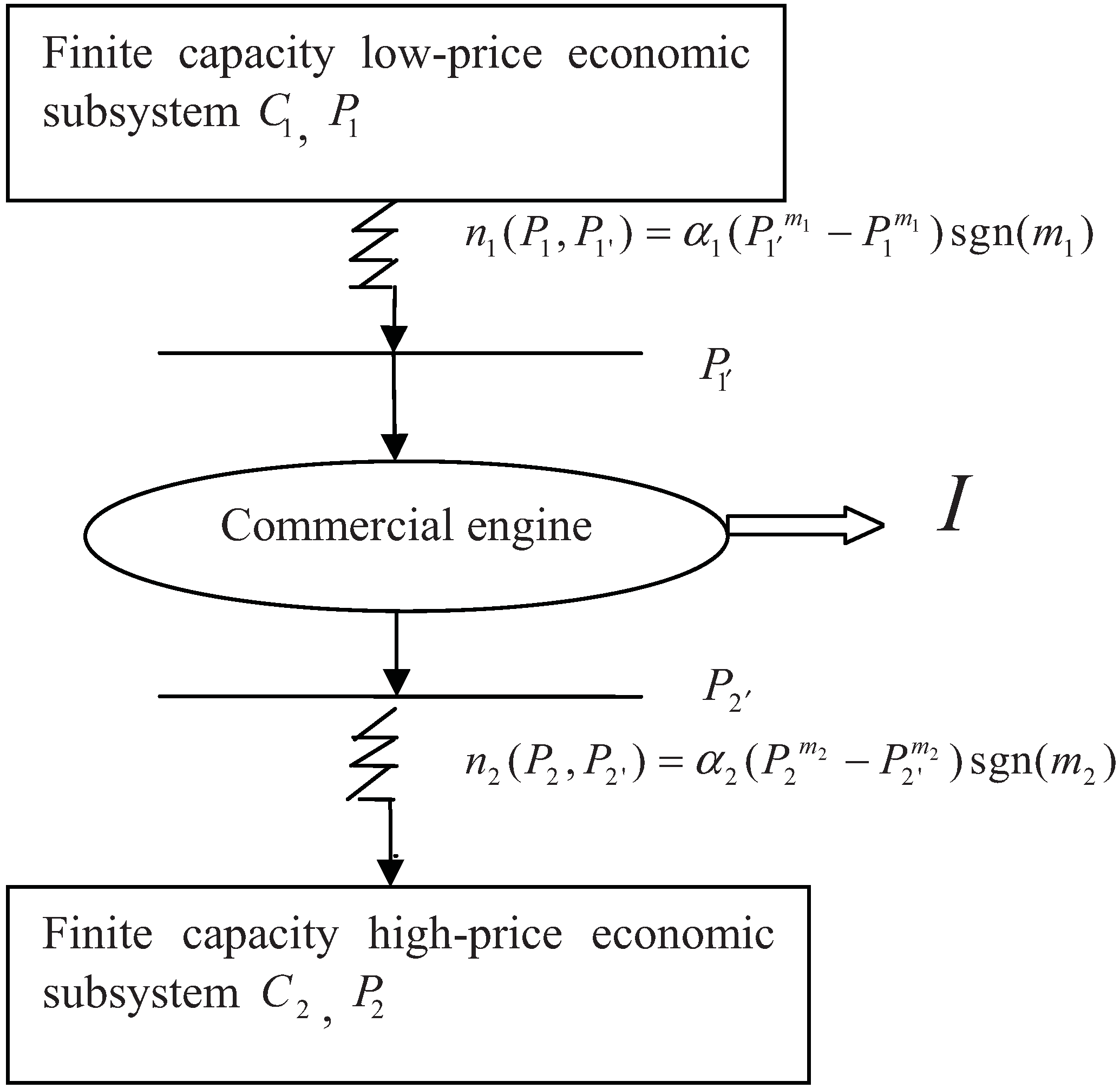
The model of the commercial engine with finite capacity low-price economic subsystem and finite capacity high-price economic subsystem is illustrated in Figure 1. Both commodity flow and money flow are present in the model; the former flows from the low-price side to the high-price side and the latter flows in the opposite direction. In this paper, commodity flow is considered and it is measured in monetary terms.
Taxation, in particular VAT (value added tax) would give similar loss terms for the monetary flows in the opposite direction. It can be seen as the heat leakage in an irreversible heat engine model [28]. In the endoreversible commercial engine model discussed herein, it is neglected just as did for the endoreversible heat engine model [26,27].
The capacity of the low-price economic subsystem is constant C1. The commodity price in the subsystem is P1, whose initial value is given by P1(0) = P10. In addition, the dynamics of P1 satisfies the equation:
which is an analogy to the dynamics of temperature of a heat reservoir with finite thermal capacity. It is a reasonable analogy because the behavior of P1 described by Equation (1) is compatible with the common assumption in economics of diminishing marginal utility. Similarly, for the finite capacity high-price subsystem, the capacity is constant C2, commodity price is P2 with initial value P2(t1) = P20 (t1 is the initial time for selling) and dynamics:
C1dP1 / dt = −dN1 / dt
C2dP2 / dt = −dN2 / dt
Figure 1.
Commercial engine model.

To consider the cases where one side or both sides have infinite capacity, one merely needs to slightly modify the results of model in this paper by taking the limit C → ∞. Furthermore, the commodity prices of the commercial engine corresponding to low-price and high-price sides are P1′ and P2′, respectively, with P1 < P1′ < P2′ < P2.
Different from the linear transfer law n ∝ Δ(P) adopted in [58], commodity flows in the present model are generalized to follow the generalized transfer law n ∝ Δ(Pm) [48,49,50]:
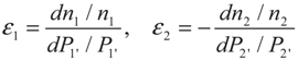
![Entropy 13 01137 i001]() where n1(P1, P1′) and n2(P2′, P2) are commodity flows corresponding to low-price and high-price sides of the commercial engine, α1(t) and α2(t) are the corresponding transfer coefficients, and exponents m1 and m2 are indicators of price elasticity of supply or demand. To elucidate, elasticity is a measure of the responsiveness of supply or demand to price changes, mathematically:
where n1(P1, P1′) and n2(P2′, P2) are commodity flows corresponding to low-price and high-price sides of the commercial engine, α1(t) and α2(t) are the corresponding transfer coefficients, and exponents m1 and m2 are indicators of price elasticity of supply or demand. To elucidate, elasticity is a measure of the responsiveness of supply or demand to price changes, mathematically:
![Entropy 13 01137 i002]()

Substituting Equation (3) into Equation (4) yields:
![Entropy 13 01137 i003]()

A one-to-one relationship between the exponent and elasticity is established above. It should be noted that m1 and m2 don’t necessarily have to be the same, because different m’s may represent different preferences of suppliers and demanders.
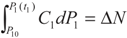
The amount of commodity exchange in the low-price side and high price side are denoted as ΔN1 and ΔN2, respectively. They are given by:
![Entropy 13 01137 i004]()
![Entropy 13 01137 i005]() where τ is the given cycle period. Additionally, market equilibrium condition requires that:
where τ is the given cycle period. Additionally, market equilibrium condition requires that:


Δ N1 = Δ N2 = Δ N
It is further assumed that purchase and selling are separate and successive processes. At time t (0 < t < t1), the commercial engine purchases commodity from the low-price subsystem; and at time t (t1 < t < τ), the commercial engine sells commodity to the high-price subsystem. Therefore, α1(t) and α2(t) have the following forms:
![Entropy 13 01137 i006]() where α1 and α2 are positive constants.
where α1 and α2 are positive constants.

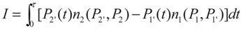
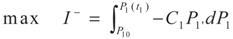
Finally, profit gained by the commercial engine is given by:
![Entropy 13 01137 i007]()
3. Optimization
The optimization problem for the commercial engine is to maximize its profit with the constraints of market equilibrium conditions and the predetermined dynamics of prices in the two economic subsystems. Mathematically, the problem amounts to determine the optimal paths of P1' and P2', the optimal values of t1 and ΔN to maximize Equation (10) subject to Equations (1), (2) and (8).
Following the method adopted in [58], optimization problem is decomposed into two sub-problems.
3.1. Problem 1


Equation (12) is obtained by substituting Equation (6) into Equation (1). Substituting Equation (12) into Equations (11) and (13) yields:
![Entropy 13 01137 i011]()
![Entropy 13 01137 i012]()
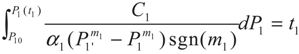
Equation (12) itself can be transformed to:
![Entropy 13 01137 i013]()
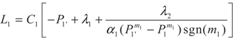
The problem now becomes maximizing Equation (14) subject to Equations (15) and (16). The corresponding modified Lagrangian function is given by:
![Entropy 13 01137 i014]() where λ1 and λ1 are Lagrangian multipliers.
where λ1 and λ1 are Lagrangian multipliers.
First order condition with respect to P1′ yields
![Entropy 13 01137 i015]() where k1 is a constant to be determined.
where k1 is a constant to be determined.

Combining Equation (18) with Equation (12) yields:
![Entropy 13 01137 i016]()
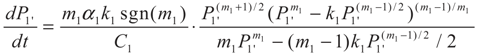
The dynamics of P1′ are uniquely characterized by Equation (19), which, combined with Equations (18), (13) and the initial value of P1, determines the paths of both P1′ and P1.
3.2. Problem 2
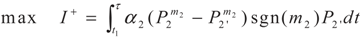


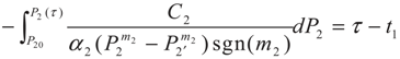
Equation (21) is obtained by substituting Equation (7) into Equation (2). Substituting Equation (21) into Equations (20) and (22) yields:
![Entropy 13 01137 i020]()
![Entropy 13 01137 i021]()


Equation (21) itself can be transformed to:
![Entropy 13 01137 i022]()
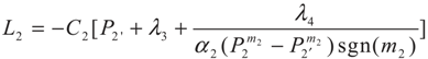
The problem now becomes maximizing Equation (23) subject to Equations (24) and (25). The corresponding modified Lagrangian function is given by:
![Entropy 13 01137 i023]() where λ3 and λ4 are Lagrangian multipliers. First order condition with respect to P2′ yields:
where λ3 and λ4 are Lagrangian multipliers. First order condition with respect to P2′ yields:
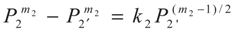
![Entropy 13 01137 i024]() where k2 is a constant to be determined.
where k2 is a constant to be determined.
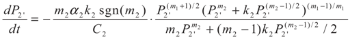
Combining Equation (27) with Equation (21) yields:
![Entropy 13 01137 i025]()
The dynamics of P2′ are uniquely characterized by Equation (28), which, combined with Equations (22), (27) and the initial value of P2, determines the paths of both P2′ and P2. In sum, the optimal paths of P1′ and P2′ are described by Equations (19) and (28). However, analytical solutions to these differential equations exist only for a few exponents such as 1 and −1. For other exponents which do not admit analytical solutions, numerical method should be adopted.
To further determine the optimal values of ΔN, t1, and I, one merely needs to substitute the paths of P1′, P1, P2′ and P2 into Equation (10) and solve the system of first order conditions.
4. Special case with m1 = 1 and m2 = 1
4.1. Analytical Solutions
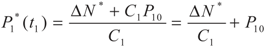
For problem 1, Equations (19), (18) and (13) are simplified to ![Entropy 13 01137 i026]() , P1′ − P1 = k1 and
, P1′ − P1 = k1 and ![Entropy 13 01137 i027]() , respectively, in this case. Solving the system gives the paths of P1 and P1′, respectively:
, respectively, in this case. Solving the system gives the paths of P1 and P1′, respectively:
 , P1′ − P1 = k1 and
 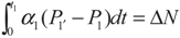 , respectively, in this case. Solving the system gives the paths of P1 and P1′, respectively:
P1 = (ΔN / C1t1)t + P10 (0 ≤ t ≤ t1)
P1′ = (ΔN / C1t1)t + P10 + ΔN / α1t1 (0 ≤ t ≤ t1)
For problem 2, Equations (28), (27) and (22) are simplified to ![Entropy 13 01137 i028]() , P2′ − P2 = k2 and
, P2′ − P2 = k2 and ![Entropy 13 01137 i029]() , respectively, in this case. Solving the system gives the paths of P2 and P2′, respectively:
, respectively, in this case. Solving the system gives the paths of P2 and P2′, respectively:
 , P2′ − P2 = k2 and
 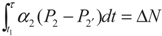 , respectively, in this case. Solving the system gives the paths of P2 and P2′, respectively:
P2 = −[ΔN / C2(τ − t1)](t − t1) + P20 (t1 ≤ t ≤ τ)
P2′ = −[ΔN / C2(τ − t1)](t − t1) + P20 − ΔN / α2(τ − t1) (t1 ≤ t ≤ τ)
Substituting Equations (29), (30), (31) and (32) into Equation (10) yields:
I = (P20 − P10)ΔN − [(1 / 2C2 + 1 / 2C1 + 1 / α2(τ − t1) + 1 / α1t1]ΔN
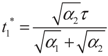
First order condition δI / δt1 = 0 yields:
![Entropy 13 01137 i030]()
Substituting Equation (29) into the First order condition δI / δ(ΔN) = 0 yields:
![Entropy 13 01137 i031]()
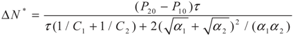
Therefore:
![Entropy 13 01137 i032]()
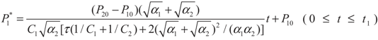
Substituting Equations (34) and (35) into Equations (29), (30), (31) and (32) yields, respectively:
![Entropy 13 01137 i033]()
![Entropy 13 01137 i034]()
![Entropy 13 01137 i035]()
![Entropy 13 01137 i036]()


4.2. Results and Discussion
It is revealed above that both P1* and P1′* increase linearly in the time, while both P2* and P2′* decrease linearly in the time; commodity flows n1(P1, P1′) and n2(P2′, P2) are constants over time; the optimal exchange time t1* is determined only by ratio of the transfer coefficients α1 and α2.
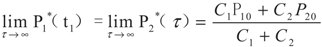
The most enlightening implication of the result is the convergence of the eventual values of P1*, P1′*, P2* and P2′*. Mathematically:
![Entropy 13 01137 i037]()

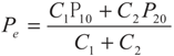
The common limit is exactly equilibrium price which completely clears the market, i.e.:
![Entropy 13 01137 i038]() which is a weighted average of the initial prices of two subsystems, and the weights are the corresponding capacities. Larger capacity indicates larger market power, therefore equilibrium price is more biased to the initial price of the party with larger capacity. Especially, if one side has infinite capacity, the equilibrium price will be the same as its initial price.
which is a weighted average of the initial prices of two subsystems, and the weights are the corresponding capacities. Larger capacity indicates larger market power, therefore equilibrium price is more biased to the initial price of the party with larger capacity. Especially, if one side has infinite capacity, the equilibrium price will be the same as its initial price.
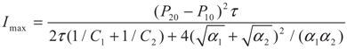
Additionally, The convergence of P1′* and P2′* also indicates that the instantaneous profit gained by the commercial engine diminishes to 0 as the cycle period approaches infinity, which further indicates that the total profit earned cannot be infinite. Equation (36) serves as an apt substantiation of this point:
![Entropy 13 01137 i039]() Finally, price convergence denies long-existing price discrepancy in a pure exchange market without exogenous interventions. Another simple but profound implication is that the profit-maximizing behavior of a commercial engine induces an optimal outcome for the market. In other words, the commercial engine, motivated by its own interest, acts as catalyst in the process of reducing price discrepancy and reaching market equilibrium. However, its existence cannot be permanent since its profit diminishes to 0 with time. In this perspective, the commercial engine can be viewed as an arbitrager whose profit-seeking action results in price parity; and the whole model simulates the dynamic process of the determination of equilibrium price.
Finally, price convergence denies long-existing price discrepancy in a pure exchange market without exogenous interventions. Another simple but profound implication is that the profit-maximizing behavior of a commercial engine induces an optimal outcome for the market. In other words, the commercial engine, motivated by its own interest, acts as catalyst in the process of reducing price discrepancy and reaching market equilibrium. However, its existence cannot be permanent since its profit diminishes to 0 with time. In this perspective, the commercial engine can be viewed as an arbitrager whose profit-seeking action results in price parity; and the whole model simulates the dynamic process of the determination of equilibrium price.
5. Special Case with m1 = − 1 and m2 = − 1
5.1. Analytical Solutions
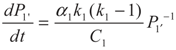
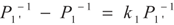
For problem 1, Equations (19), (18) and (13) are simplified to ![Entropy 13 01137 i040]() ,
, ![Entropy 13 01137 i041]() and
and ![Entropy 13 01137 i042]() , respectively. Solving the system gives the paths of P1 and P1′, respectively:
, respectively. Solving the system gives the paths of P1 and P1′, respectively:
![Entropy 13 01137 i043]()
![Entropy 13 01137 i044]()
 ,
,  and
and 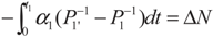 , respectively. Solving the system gives the paths of P1 and P1′, respectively:
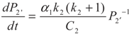
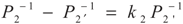
For problem 2, Equations (28), (27) and (22) are simplified to ![Entropy 13 01137 i045]() ,
, ![Entropy 13 01137 i046]() and
and ![Entropy 13 01137 i047]() , respectively. Solving the system gives the paths of P2 and P2′, respectively:
, respectively. Solving the system gives the paths of P2 and P2′, respectively:
![Entropy 13 01137 i048]()
![Entropy 13 01137 i049]()
 ,
,  and
and 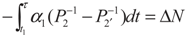 , respectively. Solving the system gives the paths of P2 and P2′, respectively:

Substituting Equations (44), (45), (46) and (47) into Equation (10) yields:
![Entropy 13 01137 i050]()

The optimal t1* and ΔN* are jointly determined by first order conditions ∂I / ∂t1 = 0 and ∂I / ∂(ΔN) = 0. However, the system of polynomials cannot be solved explicitly.
5.2. Results and Discussion
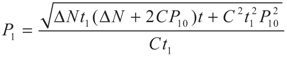
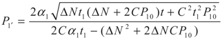
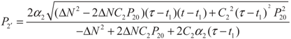
This section focuses on discussing the behaviors of P1*, P1′*, P2* and P2′* as τ →∞. From Equations (44) and (46) one can obtain:
![Entropy 13 01137 i051]()
![Entropy 13 01137 i052]()
They depend on ΔN* which cannot be solved explicitly.
To proceed, first suppose there does exist an optimal solution where P1*, P1′*, P2* and P2′* converge eventually. Then ΔN* is bounded; and thus as τ →∞, Equation (48) becomes:
![Entropy 13 01137 i053]()
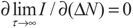
First order condition ![Entropy 13 01137 i054]() yields:
yields:
![Entropy 13 01137 i055]()
 yields:
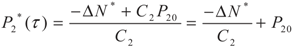
To check whether the ΔN* determined by Equation (52) supports such an optimal solution, substitute Equation (52) into Equations (49) and (50):
![Entropy 13 01137 i056]()
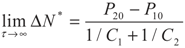
Since P1 < P1′ < P2′ < P2, there must be:
![Entropy 13 01137 i057]()

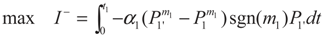
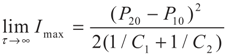
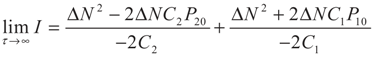
It is revealed that all four prices share common limit; therefore convergence of prices is actually an optimal solution to this problem. The corresponding maximum profit is given by:
![Entropy 13 01137 i058]()

Comparing the results of this case with m1 = m2 = −1 with those of the previous case with m1 = m2 = 1, one finds that the equilibrium price Pe, the optimal amount of commodity exchange ΔN*, and the maximum profit Imax are the same. It should be noted that this phenomenon is not a coincidence. Actually, in this model, the eventual state—market equilibrium—is solely determined by the initial conditions and the inherent characteristics of two subsystems; while the different ways of transfer (reflected by different values of m1 and m2) affect the model in respects of the specific forms of the paths of prices and the instantaneous commodity flow, i.e., the optimal configuration.
6. Conclusions
Commercial engines with finite capacity low-price economic subsystems and a generalized commodity transfer law [n ∝ Δ(Pm)] during commodity flow processes, in which the effects of the price elasticities of supply and demand are introduced, are investigated in this paper. The optimal cycle configurations of the commercial engines for maximum profit are obtained by applying optimal control theory. The optimal cycle configuration of the commercial engine with the linear transfer law [n ∝ ΔP] is that both the price estimation of finite capacity low-price economic subsystem and the commodity-buying price of the commercial engine change with time linearly and the difference between them is a constant, and the selling price of the commercial engine is a constant when it exchanges commodity with the infinite capacity high-price economic subsystem. The optimal cycle configuration of the commercial engine with the transfer law [n ∝ Δ(P−1)] is that both the price estimation of finite capacity low-price economic subsystem and the commodity-buying price of the commercial engine change with time non-linearly and the ratio between them is a constant, and the selling price of the commercial engine is a constant when it exchanges commodity with the infinite capacity high-price economic subsystem. The research in this paper further extends the research lines and methods of finite time thermodynamics to applications in fields of non-conventional thermodynamics. It is worthwhile to note that several authors [60,61,62,63,64] have criticized finite time thermodynamics (emphasis on the endoreversible model and the corresponding study results) in recent years. The responses to those articles can be seen in [65,66,67,68,69], especially, Chen et al. [67].
Acknowledgements
The author wishes to thank the reviewers for their careful, unbiased and constructive suggestions, which led to this revised manuscript.
References
- Andresen, B.; Berry, R.S.; Ondrechen, M.J.; Salamon, P. Thermodynamics for processes in finite time. Acc. Chem. Res. 1984, 17, 266–271. [Google Scholar] [CrossRef]
- Sieniutycz, S.; Salamon, P. Advances in Thermodynamics. Volume 4: Finite Time Thermodynamics and Thermoeconomics; Taylor & Francis: New York, NY, USA, 1990. [Google Scholar]
- Bejan, A. Entropy generation minimization: The new thermodynamics of finite-size device and finite-time processes. J. Appl. Phys. 1996, 79, 1191–1218. [Google Scholar] [CrossRef]
- Berry, R.S.; Kazakov, V.A.; Sieniutycz, S.; Szwast, Z.; Tsirlin, A.M. Thermodynamic Optimization of Finite Time Processes; Wiley: Chichester, UK, 1999. [Google Scholar]
- Chen, L.; Wu, C.; Sun, F. Finite time thermodynamic optimization or entropy generation minimization of energy systems. J. Non-Equil. Thermodyn. 1999, 24, 327–359. [Google Scholar] [CrossRef]
- Mironova, V.A.; Amelkin, S.A.; Tsirlin, A.M. Mathematical Methods of Finite Time Thermodynamics; Khimia: Moscow, Russia, 2000. [Google Scholar]
- Tsirlin, A.M. Optimization Methods in Thermodynamics and Microeconomics; Nauka: Moscow, Russia, 2002. [Google Scholar]
- Hoffman, K.H.; Burzler, J.; Fischer, A.; Schaller, M.; Schubert, S. Optimal process pathes for endoreversible systems. J. Non-Equil. Thermodyn. 2003, 28, 233–268. [Google Scholar] [CrossRef]
- Sieniutycz, S. Thermodynamic limits on production or consumption of mechanical energy in practical and industry systems. Progr. Energ. Combust. Sci. 2003, 29, 193–246. [Google Scholar] [CrossRef]
- Tsirlin, A.M. Irreversible Estimates of Limiting Possibilities of Thermodynamic and Microeconomic Systems; Nauka: Moscow, Russia, 2003. [Google Scholar]
- Chen, L.; Sun, F. Advances in Finite Time Thermodynamics: Analysis and optimization; Nova Science Publishers: New York, NY, USA, 2004. [Google Scholar]
- Durmayaz, A.; Sogut, O.S.; Sahin, B.; Yavuz, H. Optimization of thermal systems based on finite-time thermodynamics and thermoeconomics. Progr.s Energ. Combust. Sci. 2004, 30, 175–217. [Google Scholar] [CrossRef]
- Chen, L. Finite Time Thermodynamic Analysis of Irreversible Progresses and Cycles; High Education Press: Beijing, China, 2005. [Google Scholar]
- Tsirlin, A.M. Optimal processes in open controllable macrosystems. Autom. Rem. Contr. 2006, 67, 132–147. [Google Scholar] [CrossRef]
- de Vos, A. Thermodynamics of Solar Energy Conversion; Wiley-VCH Verlag: Berlin, Germany, 2008. [Google Scholar]
- Sieniutycz, S.; Jezowski, J. Energy Optimization in Process Systems; Elsevier: Oxford, UK, 2009. [Google Scholar]
- Curzon, F.L.; Ahlborn, B. Efficiency of a Carnot engine at maximum power output. Am. J. Phys. 1975, 43, 22–24. [Google Scholar] [CrossRef]
- Cutowicz-Krusin, D.; Procaccia, J.; Ross, J. On the efficiency of rate process: Power and efficiency of heat engines. J. Chem. Phys. 1978, 69, 3898–3906. [Google Scholar] [CrossRef]
- Ondrechen, M.J.; Rubin, M.H.; Band, Y.B. The generalized Carnot cycles: A working fluid operating in finite time between heat sources and sinks. J. Chem. Phys. 1983, 78, 4721–4727. [Google Scholar] [CrossRef]
- Chen, L.; Zhou, S.; Sun, F.; Wu, C. Optimal configuration and performance of heat engines with heat leak and finite heat capacity. Open Syst. Inform. Dynam. 2002, 9, 85–96. [Google Scholar] [CrossRef]
- Linetskii, S.B.; Tsirlin, A.M. Evaluating thermodynamic efficiency and optimizing heat exchangers. Therm. Eng. 1988, 35, 593–597. [Google Scholar]
- Andresen, B.; Gordon, J.M. Optimal heating and cooling strategies for heat exchanger design. J. Appl. Phys. 1992, 71, 76–80. [Google Scholar] [CrossRef]
- Badescu, V. Optimal strategies for steady state heat exchanger operation. J. Phys. D: Appl. Phys. 2004, 37, 2298–2304. [Google Scholar] [CrossRef]
- Xia, S.; Chen, L.; Sun, F. Optimization for entransy dissipation minimization in heat exchanger. Chin. Sci. Bull. 2009, 54, 3587–3595. [Google Scholar] [CrossRef]
- de Vos, A. Efficiency of some heat engines at maximum power conditions. Am. J. Phys. 1985, 53, 570–573. [Google Scholar] [CrossRef]
- Chen, L.; Yan, Z. The effect of heat transfer law on the performance of a two-heat-source endoreversible cycle. J. Chem. Phys. 1989, 90, 3740–3743. [Google Scholar] [CrossRef]
- Chen, L.; Sun, F.; Wu, C. The influence of heat transfer law on the endoreversible Carnot refrigerator. J. Inst. Energ. 1996, 69, 96–100. [Google Scholar]
- Chen, L.; Sun, F.; Wu, C. Effect of heat transfer law on the performance of a generalized irreversible Carnot engine. J. Phys. D: Appl. Phys. 1999, 32, 99–105. [Google Scholar] [CrossRef]
- Huleihil, M.; Andresen, B. Convective heat transfer law for an endoreversible engine. J. Appl. Phys. 2006, 100, 014911. [Google Scholar] [CrossRef]
- Yan, Z.; Chen, J. Optimal performance of a generalized Carnot cycle for another linear heat transfer law. J. Chem. Phys. 1990, 92, 1994–1998. [Google Scholar] [CrossRef]
- Chen, L.; Sun, F.; Wu, C. Optimal configuration of a two-heat-reservoir heat- engine with heat leak and finite thermal capacity. Appl. Energ. 2006, 83, 71–81. [Google Scholar] [CrossRef]
- Xiong, G.; Chen, J.; Yan, Z. The effect of heat transfer law on the performance of a generalized Carnot cycle. J. Xiamen Univ. (Nature Science) 1989, 28, 489–494. [Google Scholar]
- Chen, L.; Zhu, X.; Sun, F.; Wu, C. Optimal configurations and performance for a generalized Carnot cycle assuming the heat transfer law Q ∝ (ΔT)m. Appl. Energ. 2004, 78, 305–313. [Google Scholar] [CrossRef]
- Chen, L.; Zhu, X.; Sun, F.; Wu, C. Effect of mixed heat resistance on the optimal configuration and performance of a heat-engine cycle. Appl. Energ. 2006, 83, 537–544. [Google Scholar] [CrossRef]
- Li, J.; Chen, L.; Sun, F. Optimal configuration for a finite high-temperature source heat engine cycle with complex heat transfer law. Sci. China Ser. G 2009, 52, 587–592. [Google Scholar] [CrossRef]
- Andresen, B.; Gordon, J.M. Optimal paths for minimizing entropy generation in a common class of finite time heating and cooling processes. Int. J. Heat Fluid Flow 1992, 13, 294–299. [Google Scholar] [CrossRef]
- Badescu, V. Optimal paths for minimizing lost available work during usual heat transfer processes. J. Non-Equil. Thermodyn. 2004, 29, 53–73. [Google Scholar] [CrossRef]
- Chen, L.; Xia, S.; Sun, F. Optimal paths for minimizing entropy generation during heat transfer processes with a generalized heat transfer law. J. Appl. Phys. 2009, 105, 044907. [Google Scholar] [CrossRef]
- Xia, S.; Chen, L.; Sun, F. Optimization for minimizing lost available work during heat transfer processes with complex heat transfer law. Braz. J. Phys. 2009, 39, 98–105. [Google Scholar] [CrossRef]
- Xia, S.; Chen, L.; Sun, F. Optimal paths for minimizing entransy dissipation during heat transfer processes with generalized radiative heat transfer law. Appl. Math. Model. 2010, 34, 2242–2255. [Google Scholar] [CrossRef]
- Rozonoer, L.I. A generalized thermodynamic approach to resource exchange and allocation. I. Autom. Rem. contr. 1973, 5, 781–795. [Google Scholar]
- Rozonoer, L.I. A generalized thermodynamic approach to resource exchange and allocation. II. Autom. Rem. Contr. 1973, 6, 915–927. [Google Scholar]
- Rozonoer, L.I. A generalized thermodynamic approach to resource exchange and allocation. III. Autom. Rem. Contr. 1973, 8, 1272–1290. [Google Scholar]
- Berry, R.S.; Andresen, B. Thermodynamics constraints in economic analysis. In Self-Organization and Dissipative Structures: Applications in Physical and Social Sciences; Schieve, W.C., Allen, P.M., Eds.; University of Texas Press: Ausin, TX, USA, 1982. [Google Scholar]
- Saslow, W.M. An economic analogy to thermodynamics. Am. J. Phys. 1999, 67, 1239–1247. [Google Scholar] [CrossRef]
- Salamon, P.; Komlos, J.; Andresen, B.; Nulton, J.D. A geometric view of welfare gains with non-instantaneous adjustment. Math. Soc. Sci. 1987, 13, 153–160. [Google Scholar] [CrossRef]
- Tsirlin, A.M. Optimal control of resource exchange in economic systems. Autom. Rem. Contr. 1995, 56, 401–408. [Google Scholar]
- De Vos, A. Endoreversible thermoeconomics. Energ. Convers. Manag. 1995, 36, 1–5. [Google Scholar] [CrossRef]
- De Vos, A. Endoreversible economics. Energ. Convers. Manag. 1997, 38, 311–317. [Google Scholar] [CrossRef]
- De Vos, A. Endoreversible thermodynamics versus economics. Energ. Convers. Manag. 1999, 40, 1009–1019. [Google Scholar] [CrossRef]
- Martinas, K. About irreversibility in economics. Open Syst. Inform. Dynam. 2000, 7, 349–364. [Google Scholar] [CrossRef]
- Tsirlin, A.M. Irreversible microeconomics: optimal processes and control. Autom. Rem. Contr. 2001, 62, 820–830. [Google Scholar] [CrossRef]
- Tsirlin, A.M.; Kazakov, V.; Kolinko, N.A. Irreversibility and limiting possibilities of macrocontrolled systems: I. Thermodynamics. Open Syst. Inform. Dynam. 2001, 8, 315–328. [Google Scholar] [CrossRef]
- Tsirlin, A.M.; Kazakov, V.; Kolinko, N.A. Irreversibility and limiting possibilities of macrocontrolled systems: II. Microeconomics. Open Syst. Inform. Dynam. 2001, 8, 329–347. [Google Scholar] [CrossRef]
- Tsirlin, A.M.; Kazakov, V.A. Optimal processes in irreversible thermodynamics and microeconomics. Interdiscipl. Description Complex Syst. 2004, 2, 29–42. [Google Scholar]
- Amelkin, S.A.; Martinas, K.; Tsirlin, A.M. Optimal control for irreversible processes in thermodynamics and microeconomics. Autom. Rem. Contr. 2002, 63, 519–539. [Google Scholar] [CrossRef]
- Amelkin, S.A. Limiting possibilities of resource exchange process in complex open microeconomic system. Interdiscipl. Description Complex Syst. 2004, 2, 43–52. [Google Scholar]
- Tsirlin, A.M.; Kazakov, V. Optimal processes in irreversible microeconomics. Interdiscipl. Description Complex Syst. 2006, 4, 102–123. [Google Scholar]
- Tsirlin, A.M. Problems and methods of averaged optimization. Proc. Steklov Inst. Math. 2008, 261, 270–286. [Google Scholar] [CrossRef]
- Gyftopoulos, E.P. Fundamentals of analysis of processes. Energ. Convers. Manag. 1997, 38, 1525–1533. [Google Scholar] [CrossRef]
- Sekulic, D. P. A fallacious argument in the finite time thermodynamics concept of endoreversibility. J. Appl. Phys. 1998, 83, 4561–4565. [Google Scholar] [CrossRef]
- Moran, M.J. Proceedings of the (ECOS’98) Efficiency, Cost, Optimization, Simulation and Environmental Aspects of Energy Systems and Processes, Nancy, France, 8–10 July 1998; Bejan, A., Feidt, M., Moran, M.J., Tsatsaronis, G., Eds.; Springer: Berlin, Germany, 1998; Volume II, pp. 1147–1150.
- Moran, M.J. On second-law analysis and the failed promise of finite-time thermodynamics. Energy 1998, 23, 517–519. [Google Scholar] [CrossRef]
- Gyftopoulos, E.P. Infinite time (reversible) versus finite time (irreversible) thermodynamics: A misconceived distinction. Energy 1999, 24, 1035–1039. [Google Scholar] [CrossRef]
- Salamon, P. Physics versus engineering of finite-time thermodynamic models and optimizations. In Thermodynamic Optimization of Complex Energy Systems, NATO Advanced Study Institute, Neptun, Romania, 13—24 July 1998; Bejan, A., Mamut, E., Eds.; Kluwer Academic Publishers: The Netherlands, 1999; pp. 421–424. [Google Scholar]
- Salamon, P. A Contrast between the physical and the engineering approaches to finite-time thermodynamic models and optimizations. In Recent Advances in Finite Time Thermodynamics; Wu, C., Chen, L., Chen, J., Eds.; Nova Science Publishers: New York, NY, USA, 1999; pp. 541–552. [Google Scholar]
- Chen, J.; Yan, Z.; Lin, G.; Andresen, B. On the Curzon-Ahlborn efficiency and its connection with the efficiencies of real heat engines. Energ. Convers. Manag. 2001, 42, 173–181. [Google Scholar] [CrossRef]
- Salamon, P.; Nulton, J.D.; Siragusa, G.; Andresen, T.R.; Limon, A. Principles of control thermodynamics. Energy 2001, 26, 307–319. [Google Scholar] [CrossRef]
- Salamon, P.; Hoffmann, K.H.; Schubert, S.; Berry, R.S.; Andresen, B. What conditions make minimum entropy production equivalent to maximum power production? J. Non-Equibri. Thermodyn. 2001, 26, 73–83. [Google Scholar] [CrossRef]
© 2011 by the authors; licensee MDPI, Basel, Switzerland. This article is an open access article distributed under the terms and conditions of the Creative Commons Attribution license (http://creativecommons.org/licenses/by/3.0/).
Share and Cite
MDPI and ACS Style
Chen, Y. Maximum Profit Configurations of Commercial Engines. Entropy 2011, 13, 1137-1151. https://doi.org/10.3390/e13061137
AMA Style
Chen Y. Maximum Profit Configurations of Commercial Engines. Entropy. 2011; 13(6):1137-1151. https://doi.org/10.3390/e13061137
Chicago/Turabian StyleChen, Yiran. 2011. "Maximum Profit Configurations of Commercial Engines" Entropy 13, no. 6: 1137-1151. https://doi.org/10.3390/e13061137