Geometry of q-Exponential Family of Probability Distributions

Abstract

The Gibbs distribution of statistical physics is an exponential family of probability distributions, which has a mathematical basis of duality in the form of the Legendre transformation. Recent studies of complex systems have found lots of distributions obeying the power law rather than the standard Gibbs type distributions. The Tsallis q-entropy is a typical example capturing such phenomena. We treat the q-Gibbs distribution or the q-exponential family by generalizing the exponential function to the q-family of power functions, which is useful for studying various complex or non-standard physical phenomena. We give a new mathematical structure to the q-exponential family different from those previously given. It has a dually flat geometrical structure derived from the Legendre transformation and the conformal geometry is useful for understanding it. The q-version of the maximum entropy theorem is naturally induced from the q-Pythagorean theorem. We also show that the maximizer of the q-escort distribution is a Bayesian MAP (Maximum A posteriori Probability) estimator.

1. Introduction

Statistical physics is founded on the Gibbs distribution for microstates, which forms an exponential family of probability distributions known in statistics. Important macro-quantities such as energy, entropy, free energy, etc. are connected with it. However, recent studies show that there are non-standard complex systems which are subject to the power law instead of the exponential law of the Gibbs type distributions. See [1,2] as well as extensive literatures cited in them.

Tsallis [3] defined the q-entropy to elucidate various physical phenomena of this type, followed by many related research works on this subject (see, [1]). The concept of the q-Gibbs distribution or q-exponential family of probability distributions is naturally induced from this framework (see also [4]). However, its mathematical structure has not yet been explored enough [2,5,6], while the Gibbs type distribution has been studied well as the exponential family of distributions [7]. We need a mathematical (geometrical) foundation to study the properties of the q-exponential family. This paper presents a geometrical foundation for the q-exponential family based on information geometry [8], giving geometrical definitions of the q-potential function, q-entropy and q-divergence in a unified way.

We define the q-geometrical structure consisting of a Riemannian metric and a pair of dual affine connections. By using this framework, we prove that a family of q-exponential distributions is dually flat, in which the q-Pythagorean theorem holds. This naturally induces the corresponding q-maximum entropy theorem similarly to the case of the Tsallis q-entropy [1,9,10]. The q-structure is ubiquitous since the family $S_n$ of all discrete probability distributions can always be endowed with the structure of the q-exponential family for arbitrary q. It is possible to generalize the q-structure to any family of probability distributions. Further, it has a close relation with the α-geometry [8], which is one of information geometric structure of constant curvature. This new dually flat structure, different from the old one given rise to from the invariancy in information geometry, can be also obtained by conformal flattening of the α-geometry [11,12], using a technique in the conformal and projective geometry [13,14,15].

The present framework prepares mathematical tools for analyzing physical phenomena subject to the power law. The Legendre transformation again plays a fundamental role for deriving the geometrical dual structure. There exist lots of applications of q-geometry to information theory ([16] and others) and statistics, including Bayes q-statistics.

It is possible to generalize our framework to a more general non-linear family of distributions by using a positive convex function instead of q-exponential function (See [2,17]). A good example is the κ-exponential family [18,19,20], but we do not state it here.

2. q-Gibbs or q-Exponential Family of Distributions

2.1. q-Logarithm and q-Exponential Function

It is the first step to generalize the logarithm and exponential functions to include a family of power functions, where the logarithm and exponential functions are included as the limiting case [1,5,21]. This was also used for defining the α-family of distributions in information geometry [8]. We define the q-logarithm by

$${log}_q\left(u\right)=\frac{1}{1-q}\left(u^{1-q}-1\right),u>0$$

(1)

and its inverse function, the q-exponential, by

$${exp}_q\left(u\right)={\left\{1+(1-q)u\right\}}^{\frac{1}{1-q}},u>-1/(1-q)$$

(2)

for a positive q with $q\ne 1$. The limiting case $q\to 1$ reduces to

$$\begin{array}{ccc}\hfill {log}_1\left(u\right)& =& logu\hfill \end{array}$$

(3)

$$\begin{array}{ccc}\hfill {exp}_1\left(u\right)& =& expu\hfill \end{array}$$

(4)

so that ${log}_q$ and ${exp}_q$ are defined for $q>0$.

2.2. q-Exponential Family

The standard form of an exponential family of distributions is written as

$$p(\mathbf{x},\mathbf{\theta })=exp\left\{\sum {\theta }^i{x}_i-\psi \left(\mathbf{\theta }\right)\right\}$$

(5)

with respect to an adequate measure $\mu \left(x\right)$, where $x=\left(x_1,\cdots ,x_n\right)$ is a set of random variables and $\mathbf{\theta }=\left({\theta }^1,\cdots ,{\theta }^n\right)$ are the canonical parameters to describe the underlying system. The Gibbs distribution is of this type. Here, $\psi \left(\mathbf{\theta }\right)$ is called the free energy, which is the cumulant generating function.

The power version of the Gibbs distribution is written as

$$\begin{array}{ccc}\hfill p(x,\mathbf{\theta })& =& {exp}_q\left\{\mathbf{\theta }·x-{\psi }_q\left(\mathbf{\theta }\right)\right\}\hfill \end{array}$$

(6)

$$\begin{array}{ccc}\hfill {log}_q\left\{p(x,\mathbf{\theta })\right\}& =& \mathbf{\theta }·x-{\psi }_q\left(\mathbf{\theta }\right)\hfill \end{array}$$

(7)

where $\mathbf{\theta }·x=\sum {\theta }^i{\mathbf{x}}_i$. This is the q-Gibbs distribution or q-exponential family [4], which we denote by S, where the domain of x is restricted such that $p(x,\mathbf{\theta })>0$ holds. The function ${\psi }_q\left(\mathbf{\theta }\right)$, called the q-free energy or q-potential function, is determined from the normalization condition:

$$\int {exp}_q\left\{\mathbf{\theta }·x-{\psi }_q\left(\mathbf{\theta }\right)\right\}dx=1$$

(8)

where we replaced $d\mu \left(x\right)$ by $dx$ for brevity’s sake. The function ${\psi }_q$ depends on q, but we hereafter neglect suffix q in most cases. Research on the q-exponential family can be found, for example, in [2,4,19]. The q-Gaussian distribution is given by

$$p(\mathbf{x},\mu ,\sigma )={exp}_q\left\{-\frac{{(x-\mu )}^2}{2{\sigma }^2}-\psi (\mu ,\sigma )\right\}$$

(9)

and is studied in [22,23,24,25] in detail. Here, we need to introduce a vector random variable $x=(x,x^2)$ and a new parameter $\mathbf{\theta }$, which is a vector-valued function of μ and σ, to represent it in the standard form (7). It is an interesting observation that the domain of x in the q-Gaussian case depends on q if $0<q<1$. Hence, that q- and $q^{\prime }$-Gaussian are in general not absolutely continuous when $q\ne q^{\prime }$.

It should be remarked that the q-exponential family itself is the same as the α-family of distributions in information geometry [8]. Here, we introduce a different geometrical structure, generalizing the result of [24].

We mainly use the family $S_n$ of discrete distributions over $(n+1)$ elements $X=\left\{x_0,x_1,\cdots ,x_n\right\}$, although we can easily extend the results to the case of continuous random variables. Here, random variable x takes values over X. We also treat the case of $0<q<1$, and the limiting cases of $q=0$ or 1 give the well-known ones.

Let us put $p_i=\text{Prob}\left\{x=x_i\right\}$ and denote the probability distribution by vector $p=\left(p_0,p_1,\cdots ,p_n\right)$, where

$$\sum _{i=1}^n{p}_i=1$$

(10)

The probability of x is also written as

$$p\left(\mathbf{x}\right)=\sum _{i=0}^n{p}_i{\delta }_i\left(\mathbf{x}\right)$$

(11)

where

$${\delta }_i\left(\mathbf{x}\right)=\left\{\begin{array}{cc}1,\hfill & x=x_i,\hfill \\ 0,\hfill & \text{otherwise}.\hfill \end{array}\right.$$

(12)

Theorem 1

The family $S_n$ of discrete probability distributions has the structure of a q-exponential family for any q.

Proof 

We take ${log}_q$ of distribution $p\left(x\right)$ of (11). For any function $f\left(u\right)$, we have

$$f\left\{\sum _{i=1}^n{p}_i{\delta }_i\left(x\right)\right\}=\sum _{i=0}^{n}f\left(p_i\right){\delta }_i\left(\mathbf{x}\right)$$

(13)

By taking

$${\delta }_0\left(\mathbf{x}\right)=1-\sum _{i=1}^n{\delta }_i\left(\mathbf{x}\right)$$

(14)

into account, discrete distribution (11) can be rewritten in the form (8) as

$${log}_{q}p\left(\mathbf{x}\right)=\frac{1}{1-q}\left\{\sum _{i=1}^n\left(p_i^{1-q}-p_0^{1-q}\right){\delta }_i\left(x\right)+p_0^{1-q}-1\right\}$$

(15)

where

$$p_0=1-\sum _{i=1}^n{p}_i$$

(16)

is treated as a function of $\left(p_1,\cdots ,p_n\right)$. Hence, $S_n$ is q-exponential family (6) for any q, with the following q-canonical parameters, random variables and q-potential function:

$$\begin{array}{ccc}\hfill {\theta }^i& =& \frac{1}{1-q}\left(p_i^{1-q}-p_0^{1-q}\right),i=1,\cdots ,n\hfill \end{array}$$

(17)

$$\begin{array}{ccc}\hfill x_i& =& {\delta }_i\left(x\right)\hfill \end{array}$$

(18)

$$\begin{array}{ccc}\hfill \psi \left(\mathbf{\theta }\right)& =& -{log}_q{p}_0\hfill \end{array}$$

(19)

This completes the proof. □

Note that the q-potential $\psi \left(\mathbf{\theta }\right)$ and the canonical parameter $\mathbf{\theta }$ depend on q as is seen in (17) and (19). It should also be remarked that Theorem 1 does not contradict to the theorem 1 in [19] stating that a parametrized family of probability distributions can belong to at most one q-exponential family. The author considers an m-dimensional parametrized submanifold in $S_n$ with $m<n$ where the canonical parameter depending on q is given via the variational principle. Therefore, by denoting the q-canonical parameter by ${\mathbf{\theta }}_q\in {\mathbf{R}}^m$, we can restate his theorem in terms of geometry that a linear submanifold parametrized by ${\mathbf{\theta }}_q\in {\mathbf{R}}^m$ is not a linear submanifold parametrized by ${\mathbf{\theta }}_{q^{\prime }}\in {\mathbf{R}}^m$ when $q^{\prime }\ne q$. On the other hand, the present theorem states that there exists the q-canonical parameter ${\mathbf{\theta }}_q\in {\mathbf{R}}^n$ on whole $S_n$ for any q and the manifold has linear structure with respect to any ${\mathbf{\theta }}_q$. This is a surprising new finding.

2.3. q-Potential Function

We study the q-geometrical structure of S. The q-log-likelihood is a linear form defined by

$$l_q(\mathbf{x},\mathbf{\theta })={log}_{q}p(\mathbf{x},\mathbf{\theta })=\sum _{i=1}^n{\theta }^i{\mathbf{x}}_i-\psi \left(\mathbf{\theta }\right)$$

(20)

By differentiating it with respect to ${\theta }^i$, with the abbreviated notation ${\partial }_i=\frac{\partial }{\partial {\theta }^i}$, we have

$$\begin{array}{ccc}\hfill {\partial }_i{l}_q(x,\mathbf{\theta })& =& x_i-{\partial }_i\psi \left(\mathbf{\theta }\right)\hfill \end{array}$$

(21)

$$\begin{array}{ccc}\hfill {\partial }_i{\partial }_j{l}_q(x,\mathbf{\theta })& =& -{\partial }_i{\partial }_j\psi \left(\mathbf{\theta }\right)\hfill \end{array}$$

(22)

From this we have the following important theorem.

Theorem 2

The q-free energy or q-potential ${\psi }_q\left(\mathbf{\theta }\right)$ is a convex function of ${\mathbf{\theta }}_q$.

Proof 

We omit the suffix q for simplicity’s sake. We have

$$\begin{array}{ccc}\hfill {\partial }_{i}p(x,\mathbf{\theta })& =& p{(x,\mathbf{\theta })}^q\left(x_i-{\partial }_i\psi \right)\hfill \end{array}$$

(23)

$$\begin{array}{ccc}\hfill {\partial }_i{\partial }_{j}p(x,\mathbf{\theta })& =& qp{(x,\mathbf{\theta })}^{2q-1}\left(x_i-{\partial }_i\psi \right)\left(x_j-{\partial }_j\psi \right)-p{(x,\mathbf{\theta })}^q{\partial }_i{\partial }_j\psi \hfill \end{array}$$

(24)

The following identities hold:

$$\begin{array}{ccc}\hfill \int {\partial }_{i}p(x,\mathbf{\theta })dx& =& {\partial }_i\int p(x,\mathbf{\theta })dx=0\hfill \end{array}$$

(25)

$$\begin{array}{ccc}\hfill \int {\partial }_i{\partial }_{j}p(x,\mathbf{\theta })dx& =& {\partial }_i{\partial }_j\int p(x,\mathbf{\theta })dx=0\hfill \end{array}$$

(26)

Here, we define an important functional

$$h_q\left(\mathbf{\theta }\right)=h_q\left[p(x,\mathbf{\theta })\right]=\int p{(x,\mathbf{\theta })}^{q}dx$$

(27)

in particular for discrete $S_n$,

$$h_q\left(\mathbf{p}\right)=\sum _{i=0}^n{p}_i^q$$

(28)

for $0<q<1$. This function plays a key role in the following. From (25) and (26), by using (23) and (24), we have

$$\begin{array}{ccc}\hfill {\partial }_i\psi \left(\mathbf{\theta }\right)& =& \frac{1}{h_q\left(\mathbf{\theta }\right)}\int x_{i}p{(x,\mathbf{\theta })}^{q}dx\hfill \end{array}$$

(29)

$$\begin{array}{ccc}\hfill {\partial }_i{\partial }_j\psi \left(\mathbf{\theta }\right)& =& \frac{q}{h_q\left(\mathbf{\theta }\right)}\int \left(x_i-{\partial }_i\psi \right)\left(x_j-{\partial }_j\psi \right)p{(x,\mathbf{\theta })}^{2q-1}dx\hfill \end{array}$$

(30)

The latter shows that ${\partial }_i{\partial }_j\psi \left(\mathbf{\theta }\right)$ is positive-definite, and hence ψ is convex. □

2.4. q-Divergence

A convex function $\psi \left(\mathbf{\theta }\right)$ makes it possible to define a divergence of the Bregman-type between two probability distributions $p\left(x,{\mathbf{\theta }}_1\right)$ and $p\left(x,{\mathbf{\theta }}_2\right)$[8,26,27]. It is given by using the gradient $\nabla =\partial /\partial \mathbf{\theta }$,

$${\displaystyle D_q\left[p\left(x,{\mathbf{\theta }}_1\right):p\left(x,{\mathbf{\theta }}_2\right)\right]=}\psi \left({\mathbf{\theta }}_2\right)-\psi \left({\mathbf{\theta }}_1\right)-\nabla \psi \left({\mathbf{\theta }}_1\right)·\left({\mathbf{\theta }}_2-{\mathbf{\theta }}_1\right)$$

(31)

satisfying the non-negativity condition

$$D_q\left[p\left(x,{\mathbf{\theta }}_1\right):p\left(x,{\mathbf{\theta }}_2\right)\right]\ge 0$$

(32)

with equality when and only when ${\mathbf{\theta }}_1={\mathbf{\theta }}_2$. This gives a q-divergence in $S_n$ different from the invariant divergence of $S_n$ [28]. The divergence is canonical in the sense that it is uniquely determined in accordance with dually flat structure of q-exponential family in Section 3 and Section 4. The canonical divergence is different from the α-divergence or conventional Tsallis relative entropy used in information geometry (See the discussion in the end of this subsection). Note that it is used in [16].

Theorem 3

For two discrete distributions $p\left(x\right)=\mathbf{p}$ and $r\left(x\right)=\mathbf{r}$, the q-divergence is given by

$$D_q[\mathbf{p}:\mathbf{r}]=\frac{1}{(1-q)h_q\left(\mathbf{p}\right)}\left(1-\sum _{i=0}^n{p}_i^q{r}_i^{1-q}\right)$$

(33)

Proof 

The potentials are, from (19),

$$\psi \left(\mathbf{p}\right)=-{log}_q{p}_0,\psi \left(\mathbf{r}\right)=-{log}_q{r}_0$$

(34)

for p and r. We need to calculate $\nabla \psi \left(\mathbf{\theta }\right)$ given in (29). In our case, ${\mathbf{x}}_i={\delta }_i\left(\mathbf{x}\right)$ and hence

$${\partial }_i\psi =\frac{p_i^q}{h_q\left(\mathbf{p}\right)}$$

(35)

By using this and (17), we obtain (33). □

It is useful to consider a related probability distribution,

$${\widehat{p}}_q\left(\mathbf{x}\right)=\frac{1}{h_q\left[p\left(x\right)\right]}p{\left(x\right)}^q$$

(36)

for defining the q-expectation. This is called the q-escort probability distribution [1,4,29]. Introducing the q-expectation of random variable $f\left(x\right)$ by

$$E_{\widehat{p}}\left[f\left(x\right)\right]=\frac{1}{h_q\left[p\left(x\right)\right]}\int p{\left(x\right)}^{q}f\left(\mathbf{x}\right)dx$$

(37)

we can rewrite the q-divergence (31) for $p\left(x\right),r\left(x\right)\in S$ as

$$D_q\left[p\left(\mathbf{x}\right):r\left(\mathbf{x}\right)\right]=E_{\widehat{p}}\left[{log}_{q}p\left(x\right)-{log}_{q}r\left(x\right)\right]$$

(38)

because of the relations (20) and (29). The expression (38) is also valid on the exterior of $S\times S$ when it is integrable. This is different from the definition of the Tsallis relative entropy [30,31]

$${\tilde{D}}_q[p\left(x\right):r\left(x\right)]=\frac{1}{1-q}\left(1-\int p{\left(x\right)}^{q}r{\left(x\right)}^{1-q}dx\right)$$

(39)

which is equal to the well-known α-divergence up to a constant factor where $\alpha =1-2q$ (see [8,28]), satisfying the invariance criterion. We have

$$D_q[p\left(x\right):r\left(x\right)]=\frac{1}{h_q\left[p\left(x\right)\right]}{\tilde{D}}_q[p\left(x\right):r\left(x\right)]$$

(40)

This is a conformal transformation of divergence, as we see in the following. See also the derivation based on affine differential geometry [12].

2.5. q-Riemannian Metric

When ${\mathbf{\theta }}_2$ is infinitesimally close to ${\mathbf{\theta }}_1$, by putting ${\mathbf{\theta }}_1=\mathbf{\theta }$, ${\mathbf{\theta }}_2=\mathbf{\theta }+d\mathbf{\theta }$ and using the Taylor expansion, we have

$$D_q\left[p(\mathbf{x},\mathbf{\theta }):p(\mathbf{x},\mathbf{\theta }+d\mathbf{\theta })\right]=\sum g_{ij}^q\left(\mathbf{\theta }\right)d{\theta }^{i}d{\theta }^j$$

(41)

where

$$g_{ij}^{\left(q\right)}={\partial }_i{\partial }_j\psi \left(\mathbf{\theta }\right)$$

(42)

is a positive-definite matrix. We call $\left[g_{ij}^{\left(q\right)}\left(\mathbf{\theta }\right)\right]$ the q-Fisher information matrix. When $q=1$, this reduces to the ordinary Fisher information matrix given by

$$g_{ij}^{\left(1\right)}\left(\mathbf{\theta }\right)=g_{ij}^F\left(\mathbf{\theta }\right)=E\left[{\partial }_{i}logp(x,\mathbf{\theta }){\partial }_{j}logp(x,\mathbf{\theta })\right]$$

(43)

The positive-definite matrix $g_{ij}^{\left(q\right)}\left(\mathbf{\theta }\right)$ defines a Riemannian metric on $S_n$, giving it the q-Riemannian structure.

When a metric tensor $g_{ij}\left(\mathbf{\theta }\right)$ is transformed to

$${\tilde{g}}_{ij}\left(\mathbf{\theta }\right)=\sigma \left(\mathbf{\theta }\right)g_{ij}\left(\mathbf{\theta }\right)$$

(44)

by a positive function $\sigma \left(\mathbf{\theta }\right)$, we call it a conformal transformation. See, e.g., [13,14,15,32]. The conformal transformation of divergence induces that of the Riemannian metric.

Theorem 4

The q-Fisher information metric is given by a conformal transformation of the Fisher information metric $g_{ij}^F$ as

$$g_{ij}^{\left(q\right)}\left(\mathbf{\theta }\right)=\frac{q}{h_q\left(\mathbf{\theta }\right)}{g}_{ij}^F\left(\mathbf{\theta }\right)$$

(45)

Proof 

The q-metric is derived from the Taylor expansion of $D_q\left[p:p+dp\right]$. We have

$$\begin{array}{ccc}\hfill D_q\left[p(x,\mathbf{\theta }):p(x,\mathbf{\theta }+d\mathbf{\theta })\right]& =& \frac{1}{(1-q)h_q\left(\mathbf{\theta }\right)}\left\{1-\int p{(x,\mathbf{\theta })}^{q}p{(x,\mathbf{\theta }+d\mathbf{\theta })}^{1-q}dx\right\}\hfill \\ & =& \frac{q}{h_q\left(\mathbf{\theta }\right)}\left\{\int \frac{1}{p(x,\mathbf{\theta })}{\partial }_{i}p(x,\mathbf{\theta }){\partial }_{j}p(x,\mathbf{\theta })dx\right\}d{\theta }^{i}d{\theta }^j\hfill \end{array}$$

(46)

using the identities (25) and (26). When $q=1$, this is the Fisher information given by (43). Hence, the q-Fisher information is given by (45). □

A Riemannian metric defines the length of a tangent vector $X=\left(X^1,\cdots ,X^n\right)$ at $\mathbf{\theta }$ by

$${\parallel X\parallel }^2=\sum g_{ij}\left(\mathbf{\theta }\right)X^i{X}^j$$

(47)

Similarly, for two tangent vectors X and Y, their inner product is defined by

$$\langle X,Y\rangle =\sum g_{ij}{X}^i{Y}^j$$

(48)

When $\langle X,Y\rangle$ vanishes, X and Y are said to be orthogonal. The orthogonality, or more generally the angle, of two vectors X and Y does not change by a conformal transformation, although their magnitudes change.

3. Dually Flat Structure of q-Exponential Family

3.1. Legendre Transformation and q-Entropy

Given a convex function $\psi \left(\mathbf{\theta }\right)$, the Legendre transformation is defined by

$$\mathbf{\eta }=\nabla \psi \left(\mathbf{\theta }\right)$$

(49)

where $\nabla =\left(\partial /\partial {\theta }^i\right)$ is the gradient. Since the correspondence between $\mathbf{\theta }$ and $\mathbf{\eta }$ is one-to-one, we may consider $\mathbf{\eta }$ as another coordinate system of S.

The dual potential function is defined by

$$\phi \left(\mathbf{\eta }\right)=\underset{\mathbf{\theta }}{max}\left\{\mathbf{\theta }·\mathbf{\eta }-\psi \left(\mathbf{\theta }\right)\right\}$$

(50)

which is convex with respect to $\mathbf{\eta }$. The original coordinates are recovered from the inverse transformation given by

$$\mathbf{\theta }=\nabla \phi \left(\mathbf{\eta }\right)$$

(51)

where $\nabla =\left(\partial /\partial {\eta }_i\right)$, so that $\mathbf{\theta }$ and $\mathbf{\eta }$ are in dual correspondence.

The following theorem gives explicit relations among these quantities.

Theorem 5

The dual coordinates $\mathbf{\eta }$ are given by

$$\mathbf{\eta }=E_{\widehat{p}}\left[x\right]$$

(52)

and the dual potential is given by

$$\phi \left(\mathbf{\eta }\right)=\frac{1}{1-q}\left\{\frac{1}{h_q\left(p\right)}-1\right\}$$

(53)

Proof 

The relation (52) is immediate from (29). From the Legendre duality, the dual potential satisfies

$$\phi \left(\mathbf{\eta }\right)+\psi \left(\mathbf{\theta }\right)-\mathbf{\theta }·\mathbf{\eta }=0$$

(54)

when $\mathbf{\theta }$ and $\mathbf{\eta }$ correspond to each other by $\mathbf{\eta }=\nabla \psi \left(\mathbf{\theta }\right)$. Therefore,

$$\begin{array}{ccc}\hfill \phi \left(\mathbf{\eta }\right)& =& \sum _{i=1}^n{\theta }^i{\eta }_i-\psi \left(\mathbf{\theta }\right)\hfill \end{array}$$

(55)

$$\begin{array}{ccc}& =& E_{\widehat{p}}\left[{log}_{q}p(x,\mathbf{\theta })\right]\hfill \end{array}$$

(56)

$$\begin{array}{ccc}& =& \frac{1}{(1-q)h_q\left(\mathbf{\theta }\right)}\left(1-\int p^q(x,\mathbf{\theta })dx\right)\hfill \end{array}$$

(57)

$$\begin{array}{ccc}& =& \frac{1}{1-q}\left(\frac{1}{h_q\left(\mathbf{\theta }\right)}-1\right)\hfill \end{array}$$

(58)

This is a convex function of $\mathbf{\eta }$. □

We call the q-dual potential

$$\phi \left(\mathbf{\eta }\right)=E\left[{log}_{q}p(x,\mathbf{\theta })\right]=\frac{1}{1-q}\left\{\frac{1}{h_q}-1\right\}$$

(59)

the negative q-entropy, because it is the Legendre-dual of the q-free energy $\psi \left(\mathbf{\theta }\right)$. There are various definitions of q-entropy. The Tsallis q-entropy [3] is originally defined by

$$H_{\text{Tsallis}}=\frac{1}{1-q}\left(h_q-1\right)$$

(60)

while the Rényi q-entropy [33] is

$$H_{\text{Rényi}}=\frac{1}{1-q}log{h}_q$$

(61)

They are mutually related by monotone functions. When $q\to 1$, all of them reduce to the Shannon entropy.

Our definition of

$$H_q=\frac{1}{1-q}\left(1-\frac{1}{h_q}\right)=\frac{H_{\mathrm{Tsallis}}}{h_q}$$

(62)

is also monotonically connected with the previous ones, but is more natural from the point of view of q-geometry. The entropy $H_q$ has been known as the normalized q-entropy, which was studied in [16,34,35,36,37].

3.2. q-Dually Flat Structure

There are two dually coupled coordinate systems $\mathbf{\theta }$ and $\mathbf{\eta }$ in q-exponential family S with two potential functions $\psi \left(\mathbf{\theta }\right)$ and $\phi \left(\mathbf{\eta }\right)$ for each q. Two affine structures are introduced by the two convex functions ψ and φ. See information geometry of dually flat space [8]. Although S is a Riemannian manifold given by the q-Fisher information matrix (45), we may nevertheless regard S as an affine manifold where $\mathbf{\theta }$ is an affine coordinate system. They represent intensive quantities of a physical system. Dually, we introduce a dual affine structure to S, where $\mathbf{\eta }$ is another affine coordinate system. They represent extensive quantities. We can define two types of straight lines or geodesics in S due to the q-affine structures.

For two distributions $p\left(x,{\mathbf{\theta }}_1\right)$ and $p\left(x,{\mathbf{\theta }}_2\right)$ in S, a curve $p\left(x,\mathbf{\theta }\left(t\right)\right)$ is said to be a q-geodesic connecting them, when

$$\mathbf{\theta }\left(t\right)=t{\mathbf{\theta }}_1+(1-t){\mathbf{\theta }}_2$$

(63)

where t is the parameter of the curve. Dually, in terms of dual coordinates $\mathbf{\eta }$, when

$$\mathbf{\eta }\left(t\right)=t{\mathbf{\eta }}_1+(1-t){\mathbf{\eta }}_2$$

(64)

holds, the curve is said to be a dual q-geodesic.

More generally, the q-geodesic connecting two distribution $p_1\left(\mathbf{x}\right)$ and $p_2\left(\mathbf{x}\right)$ is given by

$${log}_{q}p(\mathbf{x},t)=t{log}_q{p}_1\left(\mathbf{x}\right)+(1-t){log}_q{p}_2\left(\mathbf{x}\right)-c\left(t\right)$$

(65)

where $c\left(t\right)$ is a normalizing term. This is rewritten as

$$p{(x,t)}^{1-q}=t{p}_1{\left(x\right)}^{1-q}+(1-t)p_2{\left(x\right)}^{1-q}-c\left(t\right)$$

(66)

Dually, the dual q-geodesic connecting $p_1\left(\mathbf{x}\right)$ and $p_2\left(\mathbf{x}\right)$ is given by using the escort distributions as

$$\widehat{p}(\mathbf{x},t)=t{\widehat{p}}_1\left(\mathbf{x}\right)+(1-t){\widehat{p}}_2\left(\mathbf{x}\right)$$

(67)

Since the manifold S has a q-Riemannian structure, the orthogonality of two tangent vectors is defined by the Riemannian metric. We rewrite the orthogonality of two geodesics in terms of the affine coordinates. Let us consider two small deviations $d_{1}p\left(\mathbf{x}\right)$ and $d_{2}p\left(\mathbf{x}\right)$ of $p\left(x\right)$, that is, from $p\left(x\right)$ to $p\left(\mathbf{x}\right)+d_{1}p\left(\mathbf{x}\right)$ and $p\left(\mathbf{x}\right)+d_{2}p\left(\mathbf{x}\right)$, which are regarded as two (infinitesimal) tangent vectors of S at $p\left(x\right)$.

Lemma 1

The inner product of two deviations $d_{1}p$ and $d_{2}p$ is given by

$$〈d_{1}p\left(x\right),d_{2}p\left(x\right)〉=\int d_1\widehat{p}\left(\mathbf{x}\right)d_2{log}_{q}p\left(\mathbf{x}\right)dx$$

(68)

Proof 

By simple calculations, we have

$$\int d_1\widehat{p}\left(\mathbf{x}\right)d_2{log}_{q}p\left(\mathbf{x}\right)dx=\frac{q}{h_q}\int \frac{d_{1}p\left(x\right)d_{2}p\left(x\right)}{p\left(x\right)}dx$$

(69)

of which the right-hand side is the Riemannian inner product in the form of (46). □

Corollary.

Two curves ${\mathbf{\theta }}_1\left(t\right)$ and ${\mathbf{\eta }}_2\left(t\right)$, intersecting at $t=0$, are orthogonal when $\langle {\dot{\mathbf{\theta }}}_1\left(0\right),{\dot{\mathbf{\eta }}}_2\left(0\right)\rangle =0$. Here, ${\dot{\mathbf{\theta }}}_1\left(t\right)$ and ${\dot{\mathbf{\eta }}}_2\left(t\right)$ denote derivatives of ${\mathbf{\theta }}_1\left(t\right)$ and ${\mathbf{\eta }}_2\left(t\right)$ by t, respectively.

The two geodesics and the orthogonality play a fundamental role in S as will be seen in the following.

4. q-Pythagorean and q-Max-Ent Theorems

A dually flat Riemannian manifold admits the generalized Pythagorean theorem and the related projection theorem [8]. We state them in our case.

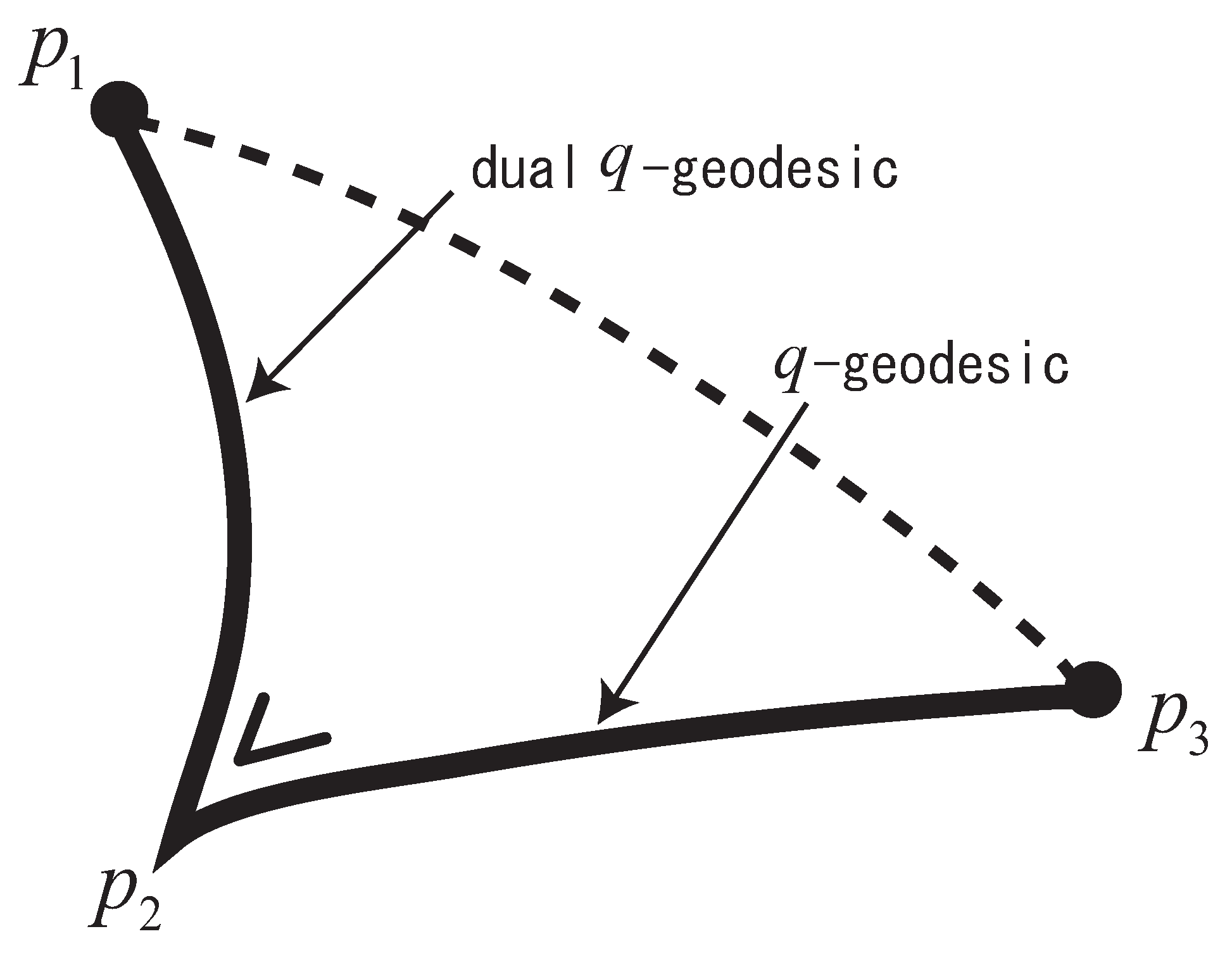
q-Pythagorean Theorem.

For three distributions $p_1\left(x\right),p_2\left(x\right)$ and $p_3\left(x\right)$ in S, it holds that

$$D_q\left[p_1:p_2\right]+D_q\left[p_2:p_3\right]=D_q\left[p_1:p_3\right]$$

(70)

when the dual geodesic connecting $p_1\left(x\right)$ and $p_2\left(x\right)$ is orthogonal at $p_2\left(x\right)$ to the geodesic connecting $p_2\left(x\right)$ and $p_3\left(x\right)$ (see Figure 1).

Figure 1. q-Pythagorean theorem.

Figure 1. q-Pythagorean theorem.

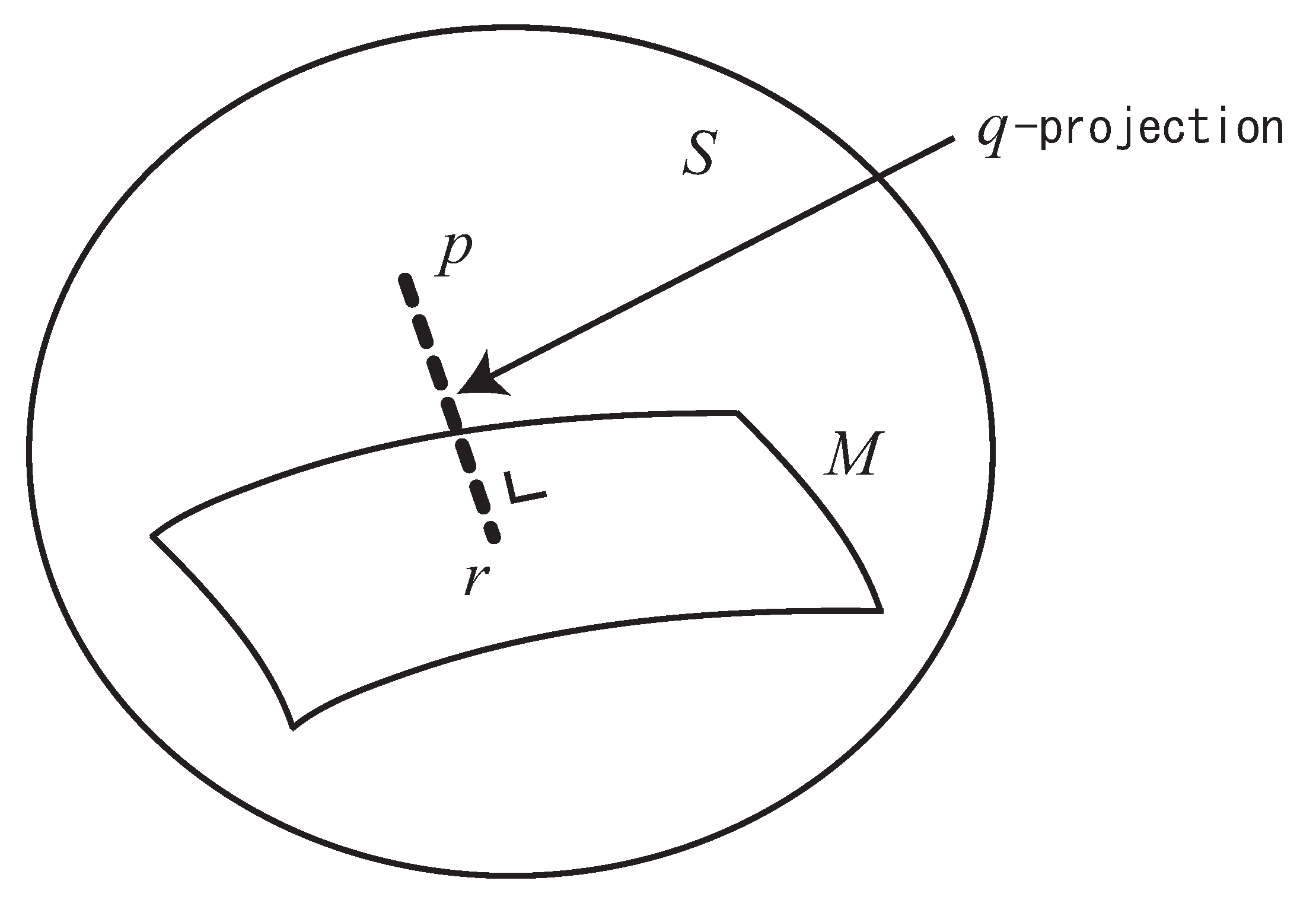
Given a distribution $p\left(x\right)\in S$ and a submanifold $M\subset S$, a distribution $r\left(x\right)\in M$ is said to be the q-projection (dual q-projection) of $p\left(x\right)$ to M, when the q-geodesic (dual q-geodesic) connecting $p\left(x\right)$ and $r\left(x\right)$ is orthogonal to M at $r\left(x\right)$ (Figure 2).

Figure 2. q-projection of p to M.

Figure 2. q-projection of p to M.

q-Projection Theorem.

Let M be a submanifold of S. Given $p\left(x\right)\in S$, the point $r\left(x\right)\in M$ that minimizes $D_q[p\left(\mathbf{x}\right):r\left(\mathbf{x}\right)]$ is given by the dual q-projection of $p\left(x\right)$ to M. The point $r\left(x\right)\in M$ that minimizes $D_q[r\left(\mathbf{x}\right):p\left(\mathbf{x}\right)]$ is given by the q-projection of $p\left(x\right)$ to M.

We show that the well-known q-max-ent theorem in the case of Tsallis q-entropy [1,4,9,11] is a direct consequence of the above q-Pythagorean and q-projection theorems.

q-Max-Ent Theorem.

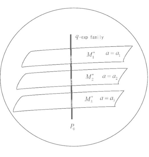
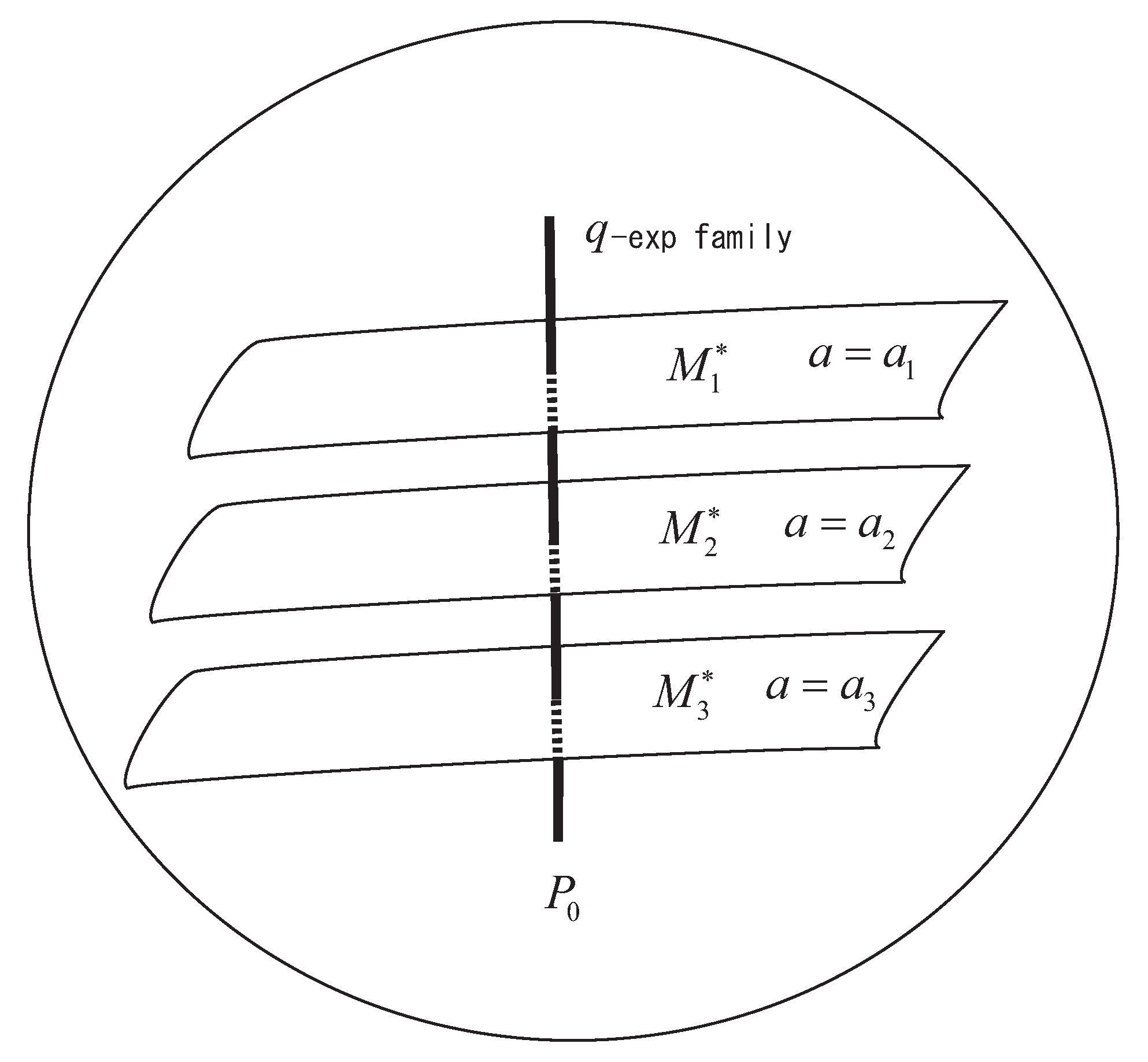
Probability distributions maximizing the q-entropies $H_{\mathrm{Tsallis}},H_{\mathrm{R}\acute{\mathrm{e}}\mathrm{nyi}}$ and $H_q$ under q-linear constraints for m random variables $c_k\left(x\right)$ and various values of $a_k$

$$E_{\widehat{p}}\left[c_k\left(\mathbf{x}\right)\right]=a_k,k=1,\cdots ,m$$

(71)

form a q-exponential family

$${log}_{q}p(x,\mathbf{\theta })=\sum _{i=1}^m{\theta }^i{c}_i\left(x\right)-\psi \left(\mathbf{\theta }\right)$$

(72)

The proof is easily obtained by the standard analytical method. Here, we give a geometrical proof. Let us consider the subspace $M^{*}\subset S$ whose member $p\left(x\right)$ satisfies the m constraints

$$E_{\widehat{p}}\left[c_k\left(\mathbf{x}\right)\right]=\int \widehat{p}\left(x\right)c_k\left(x\right)dx=a_k,k=1,\cdots ,m.$$

(73)

Since the constraints are linear in the dual affine coordinates $\mathbf{\eta }$ or $\widehat{p}\left(x\right)$, $M^{*}$ is a linear subspace of S with respect to the dual affine connection. Let $p_0(x,{\mathbf{\theta }}_0)$ be the uniform distribution defined by ${\mathbf{\theta }}_0=0$, which implies $p_0(x,{\mathbf{\theta }}_0)=\text{const}$ from (6). Let $\overline{p}\left(x\right)\in M^{*}$ be the q-projection of $p_0\left(x\right)$ to $M^{*}$ (Figure 3). Then, the divergence $D_q\left[p:p_0\right]$ from $p\left(x\right)\in M^{*}$ to $p_0\left(x\right)$ is decomposed as

$$D_q\left[p:p_0\right]=D_q\left[p:\overline{p}\right]+D_q\left[\overline{p}:p_0\right]$$

(74)

Let ${\mathbf{\eta }}_p$ be the dual coordinates of $p\left(x\right)$. Since the divergence is written as

$$D_q\left[p:p_0\right]=\psi \left({\mathbf{\theta }}_0\right)+\phi \left({\mathbf{\eta }}_p\right)-{\mathbf{\theta }}_0·{\mathbf{\eta }}_p$$

(75)

the minimizer of $D_q\left[p:p_0\right]$ among $p\left(x\right)\in M^{*}$ is just $\overline{p}\left(x\right)$, which is also the maximizer of the entropy $-\phi \left({\mathbf{\eta }}_p\right)$.

The trajectories of $\overline{p}\left(x\right)$ for various values of $a_k$ form a flat subspace orthogonal to $M^{*}$, implying that they form a q-exponential family of the form (6) (see Figure 3). The tangent directions $d\widehat{p}\left(x\right)$ of $M^{*}$ satisfies

$$\int d\widehat{p}\left(x\right)c_k\left(x\right)dx=0,k=1,\cdots ,m.$$

(76)

Hence, a q-exponential family of the form

$${log}_{q}p(x,\mathbf{\xi })=\sum _{i=1}^m{\xi }_i{d}_i\left(x\right)-\psi \left(\mathbf{\xi }\right)$$

(77)

is orthogonal to $M^{*}$, when

$$\int d\widehat{p}\left(x\right)d{log}_{q}p(x,\mathbf{\xi })dx=0$$

(78)

This implies that $d_i\left(x\right)=c_i\left(x\right)$. Hence, we have the q-exponential family (72) that maximizes the q-entropies.

Figure 3. q-Max-Ent theorem.

Figure 3. q-Max-Ent theorem.

5. q-Bayesian MAP Estimator

Given N iid observations $x_1,\cdots ,x_N$ from a statistical model $M=\left\{p(x,\mathbf{\xi })\right\}$, we have

$$p\left({\mathbf{x}}_1,\cdots ,{\mathbf{x}}_N,\mathbf{\xi }\right)=\prod _{i=1}^{N}p\left({\mathbf{x}}_i,\mathbf{\xi }\right)$$

(79)

Since ${log}_{q}u$ is a monotonically increasing function, the maximizer of the q-likelihood

$$l_q({\mathbf{x}}_1,\cdots ,{\mathbf{x}}_N,\mathbf{\xi })={log}_{q}p({\mathbf{x}}_1,\cdots ,{\mathbf{x}}_N,\mathbf{\xi })$$

(80)

is the same as the ordinary maximum likelihood estimator (mle). However, the maximizer of the q-escort distribution that maximizes the q-escort log-likelihood,

$$\frac{1}{q}\widehat{l}({\mathbf{x}}_1,\cdots ,{\mathbf{x}}_N,\mathbf{\xi })=logp({\mathbf{x}}_1,\cdots ,{\mathbf{x}}_N,\mathbf{\xi })-\frac{1}{q}log{h}_q\left(\mathbf{\xi }\right)$$

(81)

is different from this. We show that the q-mle is a Bayesian MAP (maximum a posteriori probability) estimator. This clarifies the meaning of the q-escort mle.

The q-escort mle is the maximizer of the q-escort distribution,

$${\widehat{\mathbf{\xi }}}_q=argmax\widehat{p}\left({\mathbf{x}}_1,\cdots ,{\mathbf{x}}_N,\mathbf{\xi }\right)$$

(82)

Theorem 6

The q-escort mle ${\widehat{\mathbf{\xi }}}_q$ is the Bayesian MAP estimator with the prior distribution

$$\pi \left(\mathbf{\xi }\right)=h_q{\left(\mathbf{\xi }\right)}^{-N/q}$$

(83)

Proof 

The Bayesian MAP is the maximizer of the posterior distribution with prior $\pi \left(\mathbf{\xi }\right)$

$$p\left(\mathbf{\xi }|{\mathbf{x}}_1,\cdots ,{\mathbf{x}}_N\right)=\frac{\pi \left(\mathbf{\xi }\right)p\left(x_1,\cdots ,x_N,\mathbf{\xi }\right)}{p\left(x_1,\cdots ,x_N\right)}$$

(84)

which also maximizes

$${\left(\pi \left(\mathbf{\xi }\right)p\left(x_1,\cdots ,x_N,\mathbf{\xi }\right)\right)}^q,\text{for} q>0$$

(85)

On the other hand, the q-escort mle is the maximizer of

$$\widehat{p}\left({\mathbf{x}}_1,\cdots ,{\mathbf{x}}_N,\mathbf{\xi }\right)=\prod _{i=1}^N\widehat{p}({\mathbf{x}}_i,\mathbf{\xi })=\prod _{i=1}^N\frac{p{\left(x_i,\mathbf{\xi }\right)}^q}{h_q\left(\mathbf{\xi }\right)}$$

(86)

Hence, when

$$\pi \left(\mathbf{\xi }\right)=h_q{\left(\mathbf{\xi }\right)}^{-N/q}$$

(87)

the two estimators are identical. □

The theorem shows that the Bayesian prior has a peak at the maximizer of our q-entropy $H_q$.

6. Conclusions

Much attention has been recently paid to the probability distributions subject to the power law, instead of the exponential law, since Tsallis proposed the q-entropy and related theories. The power law is also found in various communication networks. It is now a hot topic of research.

However, we do not have a geometrical foundation while that for the ordinary family of probability distributions is given by information geometry [8]. The present paper tried to give a geometrical foundation to the q-family of probability distributions. We introduced a new notion of the q-geometry. The q-structure is ubiquitous in the sense that the family of all the discrete probability distributions (and the family of all the continuous probability distributions, if we neglect delicate problems involved in the infinite dimensionality) belongs to the q-exponential family of distributions for any q. That is, we can introduce the q-geometrical structure to an arbitrary family of probability distributions, because any parametrized family of probability distributions forms a submanifold embedded in the entire manifold.

The q-structure consists of a Riemannian metric together with a pair of dually coupled affine connections, which sits in the framework of the standard information geometry. However, the q-structure is essentially different from the standard one derived by the invariance criterion of the manifold of probability distributions. We have a novel look on the theory related to the q-entropy from a viewpoint of conformal transformation. This leads us to unified definitions of various quantities such as the q-entropy, q-divergence, q-potential function and their duals, as well as new interpretations of known quantities.

This is a geometrical foundation and we expect that the paper contributes to provide further developments in this field.

References

- Tsallis, C. Introduction to Nonextensive Statistical Mechanics; Springer: New York, NY, USA, 2009. [Google Scholar]
- Naudts, J. Generalised Thermostatistics; Springer: London, UK, 2011. [Google Scholar]
- Tsallis, C. Possible generalization of Boltzmann-Gibbs statistics. J. Stat. Phys. 1988, 52, 479–487. [Google Scholar] [CrossRef]
- Naudts, J. The q-exponential family in statistical Physics. Cent. Eur. J. Phys. 2009, 7, 405–413. [Google Scholar] [CrossRef]
- Suyari, H. Mathematical structures derived from the q-multinomial coefficient in Tsallis statistics. Physica A 2006, 368, 63–82. [Google Scholar] [CrossRef]
- Suyari, H.; Wada, T. Multiplicative duality, q-triplet and μ, ν, q-relation derived from the one-to-one correspondence between the (μ, ν)-multinomial coefficient and Tsallis entropy Sq. Physica A 2008, 387, 71–83. [Google Scholar] [CrossRef]
- Barndorff-Nielsen, O.E. Information and Exponential Families in Statistical Theory; Wiley: New York, NY, USA, 1978. [Google Scholar]
- Amari, S.; Nagaoka, H. Methods of Information Geometry (Translations of Mathematical Monographs); Oxford University Press: Oxford, UK, 2000. [Google Scholar]
- Ohara, A. Geometry of distributions associated with Tsallis statistics and properties of relative entropy minimization. Phys. Lett. A 2007, 370, 184–193. [Google Scholar] [CrossRef]
- Furuichi, S. On the maximum entropy principle and the minimization of the Fisher information in Tsallis statistics. J. Math. Phys. 2009, 50, 013303. [Google Scholar] [CrossRef]
- Ohara, A. Geometric study for the Legendre duality of generalized entropies and its application to the porous medium equation. Eur. Phys. J. B 2009, 70, 15–28. [Google Scholar] [CrossRef]
- Ohara, A.; Matsuzoe, H.; Amari, S. A dually flat structure with escort probability and its application to alpha-Voronoi diagrams. In arXiv; 2010; arXiv:cond-mat/1010.4965. [Google Scholar]
- Kurose, T. On the Divergence of 1-conformally Flat Statistical Manifolds. Tôhoku Math. J. 1994, 46, 427–433. [Google Scholar] [CrossRef]
- Matsuzoe, H. Geometry of contrast functions and conformal geometry. Hiroshima Math. J. 1999, 29, 175–191. [Google Scholar]
- Kurose, T. Conformal-projective geometry of statistical manifolds. Interdisciplinary Information Sciences 2002, 8, 89–100. [Google Scholar] [CrossRef]
- Yamano, T. Information theory based on non-additive information content. Phys. Rev. E 2001, 63, 046105. [Google Scholar] [CrossRef]
- Naudts, J. Estimators, escort probabilities, and phi-exponential families in statistical physics. J. Ineq. Pure Appl. Math. 2004, 5, 102. [Google Scholar]
- Pistone, G. kappa-exponential models from the geometrical viewpoint. Eur. Phys. J. B 2009, 70, 29–37. [Google Scholar] [CrossRef]
- Naudts, J. Generalized exponential families and associated entropy functions. Entropy 2008, 10, 131–149. [Google Scholar] [CrossRef]
- Kaniadakis, G.; Lissia, M.; Scarfone, A.M. Deformed logarithms and entropies. Physica A 2004, 340, 41–49. [Google Scholar] [CrossRef]
- Yamano, T. Some properties of q-logarithmic and q-exponential functions in Tsallis statistics. Physica A 2002, 305, 486–496. [Google Scholar] [CrossRef]
- Tsallis, C.; Levy, S.V.F.; Souza, A.M.C.; Maynard, R. Statistical-mechanical foundation of the ubiquity of Levy distributions in nature. Phys. Rev. Lett. 1995, 75, 3589–3593, Erratum Phys. Rev. Lett. 1996, 77, 5442.. [Google Scholar] [CrossRef]
- Tanaka, M. A consideration on the family of q-Gaussian distributions. IEICE (Japan) 2002, J85–D2, 161–173. (in Japanese). [Google Scholar]
- Zhang, Z.; Zhong, F.; Sun, H. Information geometry of the power inverse Gaussian distribution. Appl. Sci. 2007, 9, 194–203. [Google Scholar]
- Ohara, A.; Wada, T. Information geometry of q-Gaussian densities and behaviors of solutions to related diffusion equations. J. Phys. A: Math. Theor. 2010, 43, 035002. [Google Scholar] [CrossRef]
- Wada, T. Generalized log-likelihood functions and Bregman divergences. J. Math. Phys. 2009, 50, 113301. [Google Scholar] [CrossRef]
- Cichocki, A.; Cruces, S.; Amari, S. Generalized alpha-beta divergences and their application to robust nonnegative matrix factorization. Entropy 2011, 13, 134–170. [Google Scholar] [CrossRef]
- Amari, S. α-divergence is unique, belonging to both f-divergence and Bregman divergence classes. IEEE Trans. Inform. Theor. 2009, 55, 4925–4931. [Google Scholar] [CrossRef]
- Beck, C.; Schlögl, F. Thermodynamics of Chaotic Systems; Cambridge University Press: Cambridge, UK, 1993. [Google Scholar]
- Borland, L.; Plastino, A.R.; Tsallis, C. Information gain within nonextensive thermostatistics. J. Math. Phys. 1998, 39, 6490–6501. [Google Scholar] [CrossRef]
- Furuichi, S. Fundamental properties of Tsallis relative entropy. J. Math. Phys. 2004, 45, 4868–4877. [Google Scholar] [CrossRef]
- Okamoto, I.; Amari, S.; Takeuchi, K. Asymptotic theory of sequential estimation procedures for curved exponential families. Ann. Stat. 1991, 19, 961–981. [Google Scholar] [CrossRef]
- Rényi, A. On measures of entropy and information. In Proceedings of the 4th Berkeley Symposium on Mathematics, Statistics and Probability, Berkeley, CA, USA, 20 June–30 July 1960; pp. 547–561.
- Landsberg, P.T.; Vedral, V. Distributions and channel capacities in generalized statistical mechanics. Phys. Lett. A 1998, 247, 211–217. [Google Scholar] [CrossRef]
- Rajagopal, A.K.; Abe, S. Implications of form invariance to the structure of nonextensive entropies. Phys. Rev. Lett. 1999, 83, 1711–1714. [Google Scholar] [CrossRef]
- Yamano, T. Source coding theorem based on a nonadditive information content. Physica A 2002, 305, 190–195. [Google Scholar] [CrossRef]
- Wada, T.; Scarfone, A.M. Connections between Tsallis’ formalisms employing the standard linear average energy and ones employing the normalized q-average energy. Phys. Lett. A 2005, 335, 351–362. [Google Scholar] [CrossRef]
© 2011 by the authors; licensee MDPI, Basel, Switzerland. This article is an open access article distributed under the terms and conditions of the Creative Commons Attribution license (http://creativecommons.org/licenses/by/3.0/).
Share and Cite
MDPI and ACS Style
Amari, S.-i.; Ohara, A. Geometry of q-Exponential Family of Probability Distributions. Entropy 2011, 13, 1170-1185. https://doi.org/10.3390/e13061170
AMA Style
Amari S-i, Ohara A. Geometry of q-Exponential Family of Probability Distributions. Entropy. 2011; 13(6):1170-1185. https://doi.org/10.3390/e13061170
Chicago/Turabian StyleAmari, Shun-ichi, and Atsumi Ohara. 2011. "Geometry of q-Exponential Family of Probability Distributions" Entropy 13, no. 6: 1170-1185. https://doi.org/10.3390/e13061170