Joint Markov Blankets in Feature Sets Extracted from Wavelet Packet Decompositions

Abstract

Since two decades, wavelet packet decompositions have been shown effective as a generic approach to feature extraction from time series and images for the prediction of a target variable. Redundancies exist between the wavelet coefficients and between the energy features that are derived from the wavelet coefficients. We assess these redundancies in wavelet packet decompositions by means of the Markov blanket filtering theory. We introduce the concept of joint Markov blankets. It is shown that joint Markov blankets are a natural extension of Markov blankets, which are defined for single features, to a set of features. We show that these joint Markov blankets exist in feature sets consisting of the wavelet coefficients. Furthermore, we prove that wavelet energy features from the highest frequency resolution level form a joint Markov blanket for all other wavelet energy features. The joint Markov blanket theory indicates that one can expect an increase of classification accuracy with the increase of the frequency resolution level of the energy features.

1. Introduction

Raw input variables, such as the single samples from time series or the single pixels from images, are often meaningless to the targeted audience, e.g., an industrial expert or a clinician. The ease of interpretation can be enhanced by first constructing meaningful features.

A basic approach to construct features from time series and images consists in computing some general statistical parameters such as the median, the mean, the standard deviation and higher-order moments. A more thorough approach exists in using basis functions, sometimes called templates, that can be used to construct features. The prior information about the classes to be predicted is then related to the choice of the templates. However, generic approaches that generate a library of templates, such as wavelet packets, have been proposed by Coifman and Meyer [1]. Wavelet packet decompositions (WPD’s) offer a library of templates that have many desired properties. First of all, WPD’s can be founded on the mathematical theory of multiresolution analysis [2,3] that allows to represent signals and images in new bases. The decomposition in a new wavelet packet basis guarantees that no “information” is lost as the original signals can always be reconstructed from the new basis. Secondly, the templates in a wavelet packet decomposition are easily interpreted in terms of frequencies and bandwidths [4]. Thirdly, wavelet packet decompositions are more flexible than the discrete wavelet transform and the Fourier transform. This means that the basis functions that are used in a discrete wavelet transform (DWT) are also available in the wavelet packet decomposition [3,4].

We refer here to the selection of wavelet coefficients or features derived from the wavelet coefficients to predict a target variable “C” (e.g., a class label) as feature subset selection. A basis selection algorithm specifically tuned for wavelet packet decompositions has been first proposed in [5]. This algorithm did not take into account a target variable, such as a class label, but chose one basis using minimal entropy as the selection criterion. Algorithms that take the target variable into account were proposed in [6,7,8]. It was shown [9,10] that dependencies between wavelet features were not taken into account in the previous algorithms. Dependencies between wavelet features were taken into account more recently in, e.g., [10,11,12,13]. However, a systematic analysis of redundancies between wavelet packet features by means of Markov blankets, as a solid theoretical framework to assess redundancies, is lacking so far. The dependencies between wavelet features will allow us to obtain analytical results on the existence of Markov blankets regardless of the underlying probability distribution of signals and images. In this article, we infer the redundancies between the wavelet coefficients and between energy features that are computed from a wavelet packet decomposition by means of the joint Markov blanket theory. These energy features are regularly computed from wavelet coefficients to scale down the number of features to select from as, e.g., in [12,13,14]. Other features such as the variance of the wavelet coefficients have been used in the literature as well, see, e.g., [15]. The joint Markov blankets proposed in this article are shown to be a natural result of iteratively applying Markov blanket filtering.

2. Feature Extraction from Wavelet Packet Decomposition

This section introduces the background for feature construction from wavelet packet decompositions. We will use the terminology of template and basis function interchangeably. Strictly speaking, a template is a more general terminology, because it does not need to be part of a basis. We use time series to develop the theory as it allows for a more simple notation, the results can be easily extended to images. We represent a single time series by means of a sequence of observations x(t): x(0), x(1), ... x$(N-1)$, where “t” refers to the time index and “N” is the number of samples. Time series x(t) can be considered as being sampled from an “N” dimensional distribution defined over an “N” dimensional variable X(t): X(0), X(1), ... X$(N-1)$, we write this “N” dimensional variable in shorthand notation as X${}_{\mathit{0}:\mathit{N}-\mathit{1}}$ and use capitals to denote variables.

2.1. Wavelet Coefficient Features

Features are computed from a wavelet packet decomposition by computing the inner product between the templates and the time series (using a continuous notation, for the ease of notation):

$${\gamma }_{i,j,k}=<x\left(t\right),{\psi }_i^j(t-2^{i}k)>=\underset{-\infty }{\overset{+\infty }{\int }}x\left(t\right){\psi }_i^j(t-2^{i}k)dt$$

(1)

A feature, in this case a wavelet coefficient, in the wavelet packet decomposition needs to be specified by the scale index “i”, frequency index “j” and time index “k”. The coefficient ${\gamma }_{i,j,k}$ can be considered as quantifying the similarity, by means of the inner product, between time series x(t) and wavelet function ${\psi }_i^j(t-2^{i}k)$ at position 2${}^{\mathit{i}}$k in time. The parameter “i” is the scale index and causes a dilation (commonly called a “stretching”) of the wavelet function ${\psi }^j\left(t\right)$ by a factor 2${}^{\mathit{i}}$:

$${\psi }_i^j\left(t\right)=\frac{1}{\sqrt{2^i}}{\psi }^j\left(\frac{t}{2^i}\right)$$

(2)

The wavelet functions ${\psi }_i^j\left(t\right)$ are recursively defined by means of the low-pass filter h[k] and high-pass filter g[k]:

$${\psi }_{i+1}^{2j}\left(t\right)=\sum _{-\infty }^{+\infty }h\left[k\right]{\psi }_i^j(t-2^{i}k)$$

(3)

and

$${\psi }_{i+1}^{2j+1}\left(t\right)=\sum _{-\infty }^{+\infty }g\left[k\right]{\psi }_i^j(t-2^{i}k)$$

(4)

In order to form an orthonormal system the filters h[k] and g[k] need to satisfy the conjugate mirror filter condition [3]:

$$g\left[k\right]={(-1)}^{(1-k)}h[1-k]$$

(5)

It is the parameter “j” in (2) that determines the shape of the template. In case we choose the 12-tap Coiflet filter, [16] (see pp. 258–261) we obtain the first 8 different templates ${\psi }^0\left(t\right)$, ${\psi }^1\left(t\right)$, ${\psi }^2\left(t\right)$, ... ${\psi }^7\left(t\right)$ shown in Figure 1. The construction of these basis functions can be found in text books [16].

In Figure 2, we show a graphical representation of the different subspaces that are obtained in a wavelet packet decomposition. In the discrete wavelet transform the only nodes in the tree that are considered are $W_1^1$,$W_2^1$, $W_3^1$, $W_4^1$ and $W_4^0$; these subspaces are shaded in grey.

The first four subspaces are spanned by the functions ${\left\{{\psi }_1^1(t-2k)\right\}}_{k\in \mathbb{Z}}$ , ${\left\{{\psi }_2^1(t-2^{2}k)\right\}}_{k\in \mathbb{Z}}$, ${\left\{{\psi }_3^1(t-2^{3}k)\right\}}_{k\in \mathbb{Z}}$ and ${\left\{{\psi }_4^1(t-2^{4}k)\right\}}_{k\in \mathbb{Z}}$ respectively. Subspace $W_4^0$ is spanned by ${\left\{{\psi }_4^0(t-2^{4}k)\right\}}_{k\in \mathbb{Z}}$. So in the discrete wavelet transform the signals are only analyzed by means of the time translated functions of ${\psi }_4^0\left(t\right)$ (${\psi }_0^0\left(t\right)$ is called the scaling function and is shown as the first template in Figure 1) and dilated and time translated functions of ${\psi }_0^1\left(t\right)$ (this function is called the mother wavelet function and is shown as the second template in the top row of Figure 1). The division in subspaces in Figure 2 also corresponds to a tiling of frequency space [4]. In Figure 2, only two bases are shown: the gray shaded basis corresponds with the discrete wavelet transform, the basis marked with diagonals is chosen arbitrarily and is one of the possible bases in the wavelet packet decomposition. The basis marked with diagonals puts more emphasis on a finer analysis of the higher frequency part of the signals.

Figure 1. Templates (wavelet packets) corresponding with the 12-tap Coiflet filter.

Figure 1. Templates (wavelet packets) corresponding with the 12-tap Coiflet filter.

Figure 2. Library of wavelet packet functions. Different subspaces are represented by $W_i^j$. Index “i” is the scale index, index “j” is the frequency index. The depth “I” of this tree is equal to 4. Every tree within this tree where each node has either 0 or 2 children is called an admissible tree. Two admissible trees are emphasized, one shaded in grey and one marked with diagonals. A particular node in the tree can be index by (i,j).

Figure 2. Library of wavelet packet functions. Different subspaces are represented by $W_i^j$. Index “i” is the scale index, index “j” is the frequency index. The depth “I” of this tree is equal to 4. Every tree within this tree where each node has either 0 or 2 children is called an admissible tree. Two admissible trees are emphasized, one shaded in grey and one marked with diagonals. A particular node in the tree can be index by (i,j).

Retaining any binary tree in Figure 2, where each node has either 0 or 2 children, leads to an orthonormal basis for finite energy functions, denoted as $x\left(t\right)\in L^2\left(\mathbb{R}\right)$:

$${\int }_{-\infty }^{+\infty }{\left|x\left(t\right)\right|}^{2}dt<\infty$$

(6)

Such a tree is called an admissible tree. If the leaves of this tree are denoted by ${\left\{i_l,j_l\right\}}_{1\le l\le L}$ the orthonormal system can be written as:

$$W_0^0={\oplus }_{l=1}^L{W}_{i_l}^{j_l}$$

(7)

This means that the space $W_0^0$, which is able to represent the input space of the time series, can be decomposed into orthonormal subspaces $W_{i_l}^{j_l}$.

It should be noted that a full wavelet packet decomposition yields many features. A full wavelet packet decomposition leads to N*(log${}_2$N$+1$) features. This can be seen as follows. From Figure 2, it can be noted that the number of subspaces at a certain scale “i” is determined by the scale index “i”. The number of subspaces at scale “i” is equal to 2${}^{\mathit{i}}$. Therefore the frequency index “j” at a certain scale “i” will be an integer from [0, 2${}^{\mathit{i}}$$-1$], indicating the starting position of the subspace at scale “i”. As can be seen from Equation (1) at scale “i” the inner products are computed at discrete time positions 2${}^{\mathit{i}}$k. Therefore at scale 0, we obtain “N” (length of the signals) coefficients: ${\gamma }_{0,0,0}$, ... ${\gamma }_{0,0,N-1}$. At the next scale i = 1 we obtain N/2 coefficients in each subspace i.e., ${\gamma }_{1,0,0}$, ... ${\gamma }_{1,0,N/2-1}$ and ${\gamma }_{1,1,0}$, ... ${\gamma }_{1,1,N/2-1}$. At the highest frequency resolution, i = log${}_2$N and we obtain coefficients: ${\gamma }_{logN,0,0}$, ... ${\gamma }_{logN,N-1,0}$. Hence at each scale there are “N” coefficients and in total there are log${}_2$N$+1$ different scale levels. This leads overall to N*(log${}_2$N$+1$) different coefficients to select from. When we want to emphasize the variable that can be associated with the coefficient ${\gamma }_{i,j,k}$ we use capitals ${\Gamma }_{i,j,k}$.

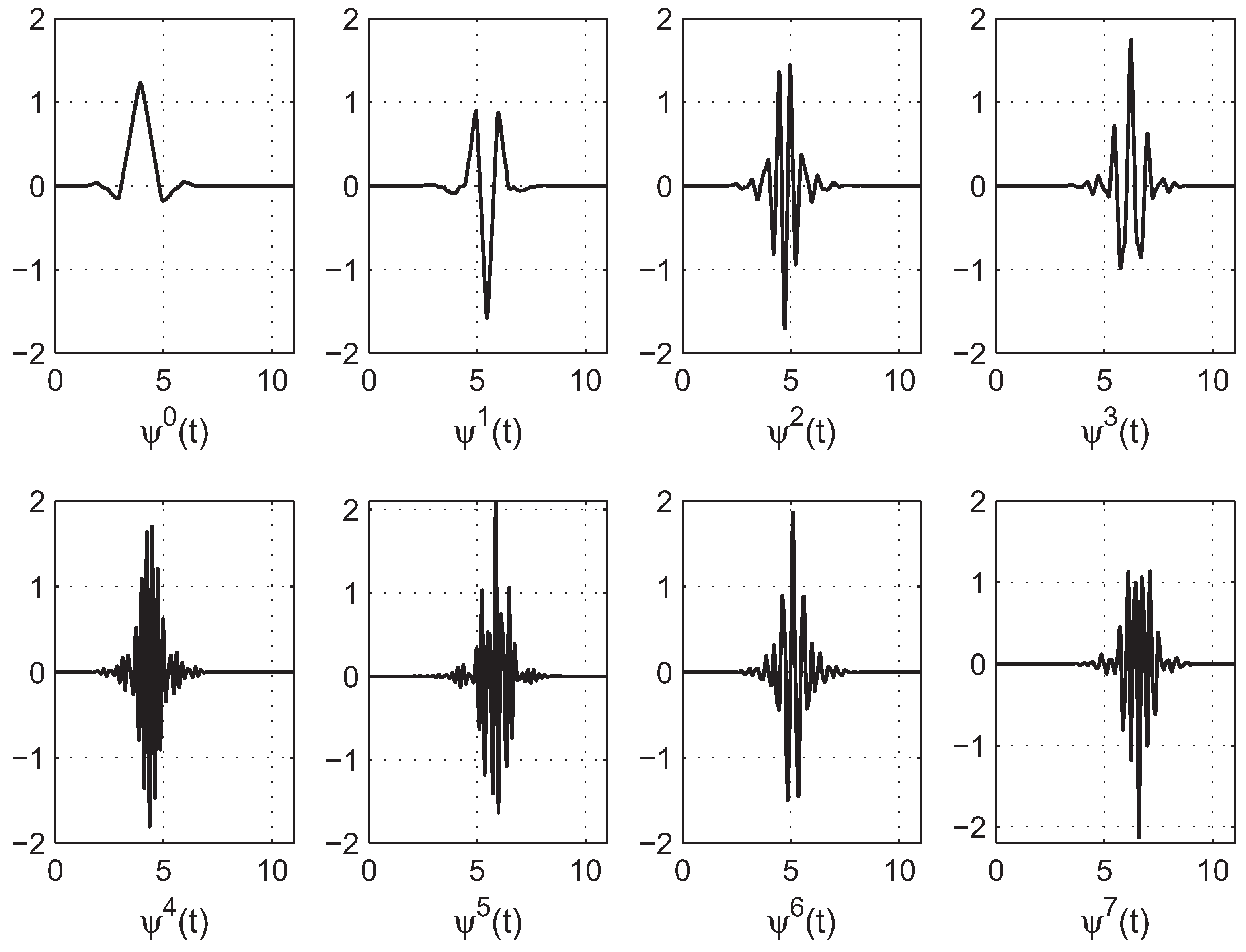
2.2. Wavelet Energy Features

In cases where one can assume that the exact time location “k” of the template is of no importance, one can, e.g., consider the energy of wavelet coefficients over time for each possible combination of the scale index “i” and the frequency index “j”:

$$E_i^j=\sum _{k=0}^{N/2^i-1}{\left({\Gamma }_{i,j,k}\right)}^2$$

(8)

Then each node in Figure 2 will correspond with 1 energy feature $E_i^j$. In total there are $\frac{1-2^{lo{g}_{2}N+1}}{1-2}=2N-1$ nodes and hence $2N-1$ energy features. Such energy features have been previously used in [8,12,13,14].

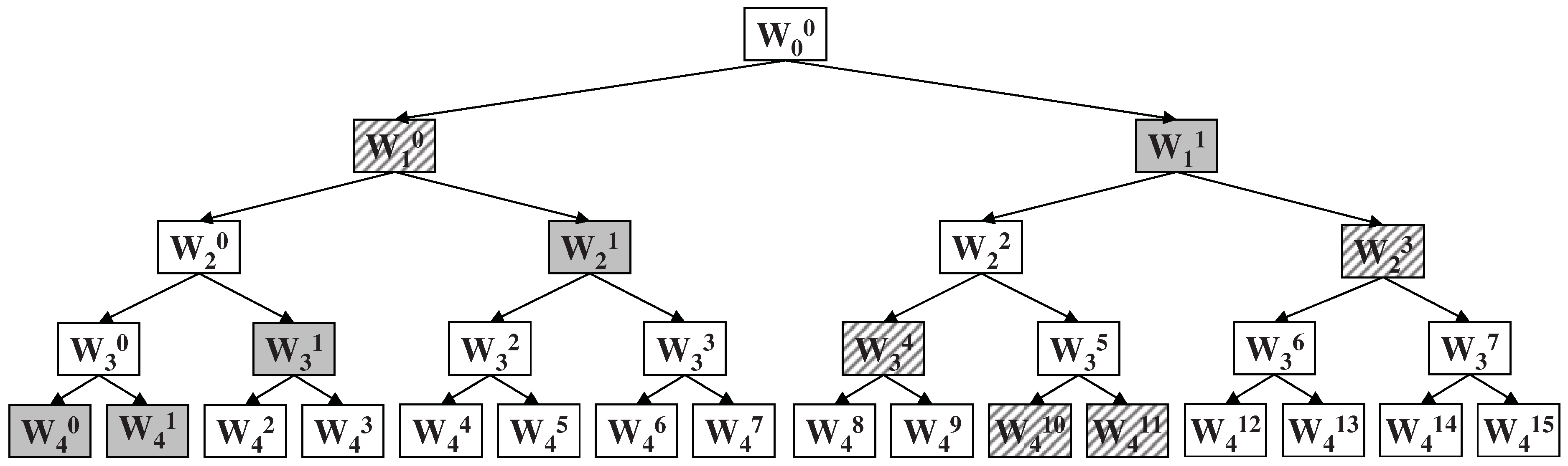
2.3. Dependencies between Wavelet Features

Analytical results of dependencies between wavelet coefficients for specific classes of stochastic signals have been obtained in [17,18] in case of fractional Brownian motion and for autoregressive models in [12]. Dependencies between wavelet packet features also exist regardless the underlying distribution of signals.

Further on, we use the notation ${\gamma }_{i,j,k}$ or ${\gamma }_{i,j}\left[k\right]$ interchangeably. The first notation emphasizes the notion as a characteristic or a feature, while the latter emphasizes the time index “k”.

Although the above definition of the wavelet coefficients ${\gamma }_{i,j,k}$ in Equation (1) allows for an intuitive interpretation as a degree of similarity, it was proven in [3] (see Proposition 8.4, p. 334) that these coefficients at the decomposition can be computed also as:

$$\begin{array}{c}\hfill {\gamma }_{i+1,2j}\left[k\right]=\sum _{m=-\infty }^{m=+\infty }{\gamma }_{i,j}\left[m\right].h[m-2k]\end{array}$$

(9)

$$\begin{array}{c}\hfill {\gamma }_{i+1,2j+1}\left[k\right]=\sum _{m=-\infty }^{m=+\infty }{\gamma }_{i,j}\left[m\right].g[m-2k]\end{array}$$

(10)

starting from the initialization: ${\gamma }_{0,0}\left[k\right]=<x\left(t\right),{\psi }_0^0(t-k)>$. Intuitively, the wavelet coefficients ${\gamma }_{i+1,2j}\left[k\right]$ can be obtained from a convolution of ${\gamma }_{i,j}\left[m\right]$ with $h[-m]$, but followed by a factor 2 subsampling. Along the same line ${\gamma }_{i+1,2j+1}\left[k\right]$ can be obtained from a convolution of ${\gamma }_{i,j}\left[m\right]$ with $g[-m]$, followed by a factor 2 subsampling. From Equation (9) and Equation (10) it is clear that level “i+1” coefficients can be computed from level “i” coefficients.

On the other hand, level “i” coefficients can also be computed from level “i+1” coefficients. At the reconstruction the coefficients can be computed as:

$$\begin{array}{c}\hfill {\gamma }_{i,j}\left[k\right]=\sum _{m=-\infty }^{m=+\infty }h[k-2m].{\gamma }_{i+1,2j}\left[m\right]+\sum _{m=-\infty }^{m=+\infty }g[k-2m].{\gamma }_{i+1,2j+1}\left[m\right]\end{array}$$

(11)

This corresponds with a convolution of $h\left[m\right]$ with ${\gamma }_{i+1,2j}\left[m\right]$, but with zeros inserted between the wavelet coefficients ${\gamma }_{i+1,2j}\left[m\right]$. The same holds for g[m] with ${\gamma }_{i+1,2j+1}\left[m\right]$.

Because wavelet packet decompositions are orthonormal transformations the energy is preserved and it holds that:

$$\begin{array}{c}\hfill E_i^j=E_{i+1}^{2j}+E_{i+1}^{2j+1}\end{array}$$

(12)

Hence, energy features at level “i” can be expressed as a sum of energy features from level “i+1”.

In order to take into account only the wavelet coefficients at scale “i” that affect wavelet coefficient ${\gamma }_{i+1,2j,k}$ at the next scale “i+1” in Equations (9) and (10), we introduce following definition.

Definition 2.1. The level “i” parent coefficients of a wavelet coefficient ${\gamma }_{i+1,2j,k}$ are the wavelet coefficients ${\gamma }_{i,j,m}$ in its parent node for which the filter coefficients h[m-2k] in Equation (9) are different from 0. Let us denote these level “i” parent features/coefficients as parent${}_i$(${\gamma }_{i+1,2j,k}$).

Similarly, the level “i” parent coefficients of a wavelet coefficient ${\gamma }_{i+1,2j+1,k}$ are the wavelet coefficients ${\gamma }_{i,j,m}$ in its parent node for which the filter coefficients g[m-2k] in Equation (10) are different from 0. These parent features are denoted as parent${}_i$(${\gamma }_{i+1,2j+1,k}$). Knowing either h[m] or g[m] these parent relationships can be derived for each level “i”.

In case of the L-tap Coiflet filters [16], the low-pass and high-pass filters consist of L filter taps each. Given the low-pass filters h[m] for the Coiflet filters in [16], it can be shown (using Equations (5), (9) and (10)) that the parents of ${\gamma }_{i+1,2j,k}$ from level “i” are the L consecutive coefficients ${\gamma }_{i,j,2k-2L/6}$, ${\gamma }_{i,j,2k-2L/6+1}$, ...${\gamma }_{i,j,2k+4L/6-1}$, see Figure 3. The parents of ${\gamma }_{i+1,2j+1,k}$ are the L consecutive coefficients ${\gamma }_{i,j,2k-(4L/6-2)}$, ${\gamma }_{i,j,2k-(4L/6-3)}$, ...${\gamma }_{i,j,2k+2L/6+1}$, see Figure 4.

Figure 3. Parent coefficient relationships for ${\gamma }_{i+1,2j,k}$.

Figure 3. Parent coefficient relationships for ${\gamma }_{i+1,2j,k}$.

Figure 4. Parent coefficient relationships for ${\gamma }_{i+1,2j+1,k}$.

Figure 4. Parent coefficient relationships for ${\gamma }_{i+1,2j+1,k}$.

Here we used the notations parent${}_i$(${\gamma }_{i+1,2j,k}$) and parent${}_i$(${\gamma }_{i+1,2j+1,k}$) to emphasize that the parent coefficients of the even frequencies ${\gamma }_{i+1,2j,k}$ and the parent coefficients of the odd frequencies ${\gamma }_{i+1,2j+1,k}$ may differ, as can be seen from Figure 3 and Figure 4. More generally (without emphasizing differences between odd and even frequency components), we can write the parents of ${\gamma }_{i,j,k}$ as: parent${}_{i-1}$(${\gamma }_{i,j,k}$).

Similarly, we introduce the child coefficients of ${\gamma }_{i,j,k}$ as the coefficients at the next resolution level “i+1” that affect ${\gamma }_{i,j,k}$.

Definition 2.2. The level “i+1” child coefficients of a wavelet feature ${\gamma }_{i,j,k}$ are the wavelet coefficients ${\gamma }_{i+1,2j,m}$ and ${\gamma }_{i+1,2j+1,m}$ in its child nodes for which the filter coefficients h[k-2m] and g[k-2m] in Equation (11) are different from 0. Let us denote these level “i+1” child features/coefficients as child${}_{i+1}$(${\gamma }_{i,j,k}$).

Note that we used the terminology of parent and child nodes as used in wavelet packet trees, these should not be confused with the terminology used in directed acyclic graphs (DAG’s).

Given the low-pass filters h[m] for the Coiflet filters in [16], it can be shown that for the L-tap Coiflet filters the child coefficients of ${\gamma }_{i,j,2k}$ from level “i+1” are the L/2 consecutive coefficients ${\gamma }_{i+1,2j,k-(2L/6-1)}$, ${\gamma }_{i+1,2j,k-(2L/6-2)}$, ...${\gamma }_{i+1,2j,k+L/6}$ and the L/2 consecutive coefficients ${\gamma }_{i+1,2j+1,k-L/6}$, ${\gamma }_{i+1,2j+1,k-L/6+1}$, ...${\gamma }_{i+1,2j+1,k+(2L/6-1)}$ (using Equation (5) and Equation (11)). The child coefficients for ${\gamma }_{i,j,2k+1}$ are the same coefficients in case of the L-tap Coiflet filters. These child coefficients are shown in Figure 5.

In Figure 5, we used a notation ${\gamma }_{i,j,2k}$ to indicate that each child node ${\gamma }_{i+1,2j,m}$ and ${\gamma }_{i+1,2j+1,m}$ only consists of half the number of coefficients. More generally, we write the child coefficients of ${\gamma }_{i,j,k}$ as child${}_{i+1}$(${\gamma }_{i,j,k}$).

Figure 5. Child coefficient relationships for ${\gamma }_{i,j,2k}$. The child coefficients for ${\gamma }_{i,j,2k+1}$ are the same coefficients in case of L-tap Coiflet filters. The top row coefficients are the odd frequency child coefficients, the bottom row are the even frequency child coefficients.

Figure 5. Child coefficient relationships for ${\gamma }_{i,j,2k}$. The child coefficients for ${\gamma }_{i,j,2k+1}$ are the same coefficients in case of L-tap Coiflet filters. The top row coefficients are the odd frequency child coefficients, the bottom row are the even frequency child coefficients.

3. Markov Blanket Filtering: A Link with Information-Theoretic Approaches

Markov blanket filtering as an approach to feature elimination was established by [19] and inspired others in the design of new feature subset selection algorithms such as in [20,21,22]. Most recent research aims at finding the Markov boundary (the minimal Markov blanket) of the target variable in feature sets containing more than ten thousands of variables while still remaining theoretically correct under the faithfulness condition [23,24,25]. A seemingly different approach to feature subset selection is that by means of mutual information that was used in [10,26,27,28,29,30,31,32]. As opposed to Markov blanket filtering, which is due to [19], the origin of the use of mutual information as a feature subset selection criterion is more unclear. We believe that the first use of mutual information as a feature subset selection criterion can be traced back to Lewis [33]. However, at that time Lewis did not call the functional used in [33] “mutual information”. A connection between Markov blanket filtering and the mutual information feature subset selection criterion was shown independently in [11] an [34].

Previous work using mutual information in [29] has used heuristic concepts of information relevance and redundancy in feature subset selection, as opposed to the statistical concepts of relevance in [35] and redundancy in [21] that can be used to obtain optimal subsets. If one makes a statement that: “a feature is redundant for a feature set with respect to the target variable”, we want to be sure that really all information about the target variable is covered in that feature set and the considered feature can be removed without information loss. This is exactly what Markov blanket filtering offers and the reason we extended it here to joint Markov blankets for inference of redundancies between features extracted from wavelet packet decompositions.

Let F${}_G$ be the current feature set, i.e., the feature set obtained after removal of some other features from the full feature set F, and $F_i$ a feature to be removed from the current feature set F${}_G$.

Definition 3.1 ([19,21]). A feature subset $M_i\subset {\mathbf{F}}_G$ is a Markov blanket for feature $F_i$ iff (if and only if): $p({\mathbf{F}}_G\setminus \{M_i\cup F_i\},C|F_i,M_i)=p({\mathbf{F}}_G\setminus \{M_i\cup F_i\},C|M_i)$.

Hence, a Markov blanket $M_i$ is a feature subset not including $F_i$ that makes $F_i$ independent of all other features ${\mathbf{F}}_G\setminus \{M_i\cup F_i\}$ and the target variable “C”: ${\mathbf{F}}_G\setminus \{M_i\cup F_i\}$∪ C. The connection with the mutual information functional [36] is given in the following, see also [11,34,37]. Read $MI(X;Y|Z)$ as the mutual information between X and Y conditioned on Z, where X, Y and Z may be single variables or sets of variables.

Lemma 3.2. A feature subset $M_i\subset {\mathbf{F}}_G$ is a Markov blanket for feature $F_i$ iff: $MI(F_i;C,{\mathbf{F}}_G\setminus \{M_i\cup F_i\}|M_i)=0$.

Proof. The comparison of the probability functions $p({\mathbf{F}}_G\setminus \{M_i\cup F_i\},C|F_i,M_i)$ and $p({\mathbf{F}}_G\setminus \{M_i\cup F_i\},C|M_i)$ is performed in information-theoretic sense by means of the Kullback-Leibler distance:

$$\sum _{{\mathbf{f}}_G,c}p({\mathbf{f}}_G,c)ln\left(\frac{p({\mathbf{f}}_G\setminus \{m_i\cup f_i\},c|f_i,m_i)}{p({\mathbf{f}}_G\setminus \{m_i\cup f_i\},c|m_i)}\right)$$

(13)

using conditional probabilities this can be written as:

$$=\sum _{{\mathbf{f}}_G,c}p({\mathbf{f}}_G,c)ln\left(\frac{p({\mathbf{f}}_G\setminus \left\{m_i\right\},c|m_i)}{p({\mathbf{f}}_G\setminus \{m_i\cup f_i\},c|m_i).p\left(f_i\right|m_i)}\right)$$

(14)

using the definition of conditional mutual information [36] this is equivalent to:

$$=MI(F_i;{\mathbf{F}}_G\setminus \{M_i\cup F_i\},C|M_i)$$

(15)

Using a corollary of the information inequality Theorem (2.6.3) in [36], it is known that the conditional mutual information in this case $MI(F_i;{\mathbf{F}}_G\setminus \{M_i\cup F_i\},C|M_i)$ is equal to 0 iff $p({\mathbf{F}}_G\setminus \{M_i\cup F_i\},C|F_i,M_i)$ = $p({\mathbf{F}}_G\setminus \{M_i\cup F_i\},C|M_i)$. □

This result can be related to Theorem 8 in [37]. There it was shown for discrete features $F_i$ that if $MI(M_i;F_i)=H\left(F_i\right)$ then $M_i$ is a Markov blanket for $F_i$. This can also be easily shown from Lemma 3.2. Starting from $MI(F_i;C,{\mathbf{F}}_G\setminus \{M_i\cup F_i\}|M_i)$, this can be written as:

$$\begin{array}{ccc}& & MI(F_i;C,{\mathbf{F}}_G\setminus \{M_i\cup F_i\}|M_i)=\hfill \\ \mathrm{(16)}& & & H\left(F_i\right|M_i)-H\left(F_i\right|M_i,C,{\mathbf{F}}_G\setminus \{M_i\cup F_i\})\hfill \end{array}$$

Using the condition $MI(M_i;F_i)=H\left(F_i\right)$ from Theorem 8 in [37] then it holds that $H\left(F_i\right|M_i)=0$. Furthermore, because conditioning reduces entropy it holds that $H\left(F_i\right|M_i,C,{\mathbf{F}}_G\setminus \{M_i\cup F_i\})\le H\left(F_i\right|M_i)$. Because Theorem 8 in [37] assumes discrete features, entropy must be ≥ 0, from which it follows that $H\left(F_i\right|M_i,C,{\mathbf{F}}_G\setminus \{M_i\cup F_i\})=0$. Hence, we obtain that $MI(F_i;C,{\mathbf{F}}_G\setminus \{M_i\cup F_i\}|M_i)=0$. This proves the Markov blanket condition. The main difference between Lemma 3.2 and Theorem 8 of [37] is that we do not need to assume discrete features.

It needs to be remarked that when dealing with small sample sizes, it has been shown [38] that Markov blanket filtering may favor the removal of features that are most correlated with the target variable. Of course, this is the opposite result of what one wants to achieve with Markov blanket filtering. In [38] this behavior was observed when discretizing the features. It still remains to be explored if such behavior can also be observed when one uses the continuous features instead.

Markov blanket filtering leads naturally to the definition of a “joint” Markov blanket $M_{S_{1:n-1}}$ of a set of features $F_{1:n-1}=$$F_1$∪$F_2$...∪$F_{n-1}$ (in information-theoretic sense):

Definition 3.3. A feature subset $M_{S_{1:n-1}}\subset \mathbf{F}$ is a joint Markov blanket for features $F_{1:n-1}=$$F_1$∪$F_2$ ...∪ $F_{n-1}$ iff: $MI(F_{1:n-1};\mathbf{F}\setminus \{F_{1:n-1}\cup M_{S_{1:n-1}}\},C|M_{S_{1:n-1}})=0$.

In the future of this article we will use a shorthand notation in the definition of the joint Markov blanket: $MI(F_{1:n-1};\mathbf{F}\setminus \{F_{1:n-1}\cup M_{S_{1:n-1}}\},C|M_{S_{1:n-1}})=0$, because conditioning is on $M_{S_{1:n-1}}$, this is equivalent to $MI(F_{1:n-1};\mathbf{F}\setminus F_{1:n-1},C|M_{S_{1:n-1}})=0$, where the latter equation is called the shorthand notation.

We show that joint Markov blankets are obtained from performing Markov blanket filtering iteratively.

Theorem 3.4. If $M_{S_{1:n-1}}$ is a joint Markov blanket for features $F_{1:n-1}=$$F_1$∪$F_2$ ...∪$F_{n-1}$ and $M_n$ is a Markov blanket for feature $F_n$ then $M_{S_{1:n-1}}$∪$M_n$ is a joint Markov blanket for $F_{1:n-1}$∪$F_n$.

Proof. We need to show that it follows from $MI(F_{1:n-1};C,\mathbf{F}\setminus F_{1:n-1}|M_{S_{1:n-1}})=0$ (i.e., $M_{S_{1:n-1}}$ is a joint Markov blanket for features $F_{1:n-1}$) and from $MI(F_n;C,\mathbf{F}\setminus \{F_{1:n-1}\cup F_n\}|M_n)=0$ (i.e., $M_n$ is a Markov blanket for feature $F_n$) then it follows that $MI(F_{1:n-1}\cup F_n;C,\mathbf{F}\setminus \{F_{1:n-1}\cup F_n\}|M_{S_{1:n-1}}\cup M_n)=0$.

Using the chain rule for information [36] (Theorem 2.5.2) we can write:

$$\begin{array}{ccc}& & MI(F_{1:n-1}\cup F_n;C,\mathbf{F}\setminus \{F_{1:n-1}\cup F_n\}|M_{S_{1:n-1}}\cup M_n)=\hfill \end{array}$$

(17)

$$\begin{array}{ccc}& & MI(F_{1:n-1};C,\mathbf{F}\setminus \{F_{1:n-1}\cup F_n\}|M_{S_{1:n-1}}\cup M_n\cup F_n)\hfill \end{array}$$

(18)

$$\begin{array}{ccc}& & +MI(F_n;C,\mathbf{F}\setminus \{F_{1:n-1}\cup F_n\}|M_{S_{1:n-1}}\cup M_n)\hfill \end{array}$$

(19)

Now we show that both (18) and (19) are equal to 0.

For (18), applying the chain rule for information to (18) we obtain:

$$\begin{array}{ccc}& & MI(F_{1:n-1};C,\mathbf{F}\setminus \{F_{1:n-1}\cup F_n\}|M_{S_{1:n-1}}\cup M_n\cup F_n)=\hfill \end{array}$$

$$\begin{array}{ccc}& & MI(F_{1:n-1};C,\mathbf{F}\setminus F_{1:n-1}|M_{S_{1:n-1}}\cup M_n\cup F_n)=\hfill \end{array}$$

(20)

$$\begin{array}{ccc}& & MI(F_{1:n-1};C,\mathbf{F}\setminus F_{1:n-1}|M_{S_{1:n-1}})-MI(F_{1:n-1};M_n\cup F_n|M_{S_{1:n-1}})\hfill \end{array}$$

(21)

In (20) the feature $F_n$ is included in $\mathbf{F}\setminus \{F_{1:n-1}\cup F_n\}$; this does not change the dependencies because conditioning is also on $F_n$. Both terms in (21) are equal to 0 zero because $M_{S_{1:n-1}}$ is a joint Markov blanket for $F_{1:n-1}$ with respect to $C\cup \mathbf{F}\setminus F_{1:n-1}$. By definition $M_{S_{1:n-1}}$ will make $F_{1:n-1}$ independent of $C\cup \mathbf{F}\setminus F_{1:n-1}$: $MI(F_{1:n-1};C,\mathbf{F}\setminus F_{1:n-1}|M_{S_{1:n-1}})=0$ (the first term in (21)) and any possible subset thereof so that: $MI(F_{1:n-1};M_n\cup F_n|M_{S_{1:n-1}})=0$ (in the second term $M_n\cup F_n\subset \mathbf{F}\setminus F_{1:n-1}$).

For (19), applying the chain rule for information on (19) we obtain:

$$\begin{array}{ccc}& & MI(F_n;C,\mathbf{F}\setminus \{F_{1:n-1}\cup F_n\}|M_{S_{1:n-1}}\cup M_n)=\hfill \end{array}$$

$$\begin{array}{ccc}& & MI(F_n;C,\mathbf{F}\setminus \{F_{1:n-1}\cup F_n\}|M_n)-MI(F_n;M_{S_{1:n-1}}|M_n)\hfill \end{array}$$

(22)

Both terms in (22) are equal to 0 because $M_n$ is a Markov blanket for $F_n$ w.r.t. $C\cup \mathbf{F}\setminus \{F_{1:n-1}\cup F_n\}$. This implies $MI(F_n;C,\mathbf{F}\setminus \{F_{1:n-1}\cup F_n\}|M_n)=0$ by definition of a Markov blanket and $MI(F_n;M_{S_{1:n-1}}|M_n)=0$ because $M_{S_{1:n-1}}$ is a subset of $\mathbf{F}\setminus \{F_{1:n-1}\cup F_n\}$. Hence, Equation (17) is equal to 0 and the condition of a “joint” Markov blanket is fulfilled. □

The proof was provided in case the feature to be removed $F_n$ was not part of the joint Markov blanket found so far $M_{1:n-1}$. More generally, one may choose $F_n$ ∈ $M_{1:n-1}$. The proof in this case becomes more elaborate, but in a similar way as above, it can be shown that the joint Markov blanket in this case becomes {$M_{1:n-1}$ ∖ $F_n$} ∪ $M_n$, with $M_n$ a Markov blanket for $F_n$. For details on the extended proof when $F_n$ ∈ $M_{1:n-1}$ the reader is referred to Theorem 2.4 in [11].

In Markov blanket filtering [19], one starts with removing a single feature based on a Markov blanket found for that feature. Hence, in order to show that iteratively performing Markov blanket filtering leads to a “joint” Markov blanket for the removed features, we need to show that according to Theorem 3.4 that the first Markov blanket found in Markov blanket filtering is a “joint” Markov blanket. Suppose that one finds a Markov blanket $M_1$ for $F_1$: for this feature $F_1$ it holds that $MI(F_1;C,\mathbf{F}\setminus \{M_1\cup F_1\}|M_1)=0$. In order for $M_1$ to be a joint Markov blanket it must satisfy: $MI(F_{1:n-1};C,\mathbf{F}\setminus F_{1:n-1}|M_{S_{1:n-1}})=0$. If we set n = 2 in the last condition we obtain: $MI(F_{1:2-1};C,\mathbf{F}\setminus F_{1:2-1}|M_{S_{1:2-1}})=0$, which can be further simplified to $MI(F_{1:1};C,\mathbf{F}\setminus F_{1:1}|M_{S_{1:1}})=0$. With $F_{1:1}=F_1\cup F_1=F_1$ , and $M_{S_{1:1}}=M_1$, we obtain: $MI(F_1;C,\mathbf{F}\setminus F_1|M_1)=0$. This condition is satisfied and hence the first Markov blanket is a special case of a joint Markov blanket. Therefore iteratively performing Markov blanket filtering leads to “joint” Markov blankets.

4. Joint Markov Blankets in Wavelet Feature Sets

We show the existence of Markov blankets in feature sets extracted from wavelet packet decompositions. In Section 4.1 the set of all features F consists of the wavelet coefficient variables ${\Gamma }_{i,j,k}$, in Section 4.2 the set consists of all energy features $E_i^j$.

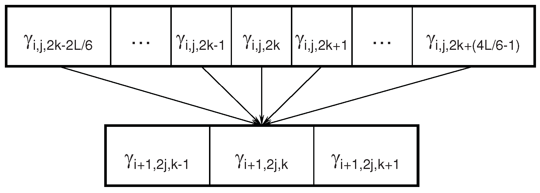
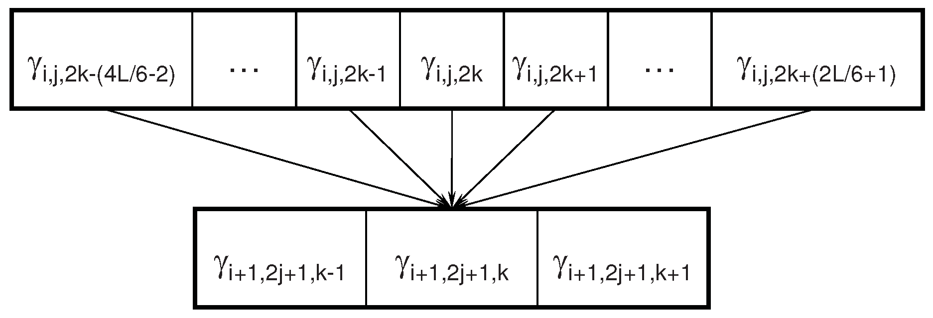
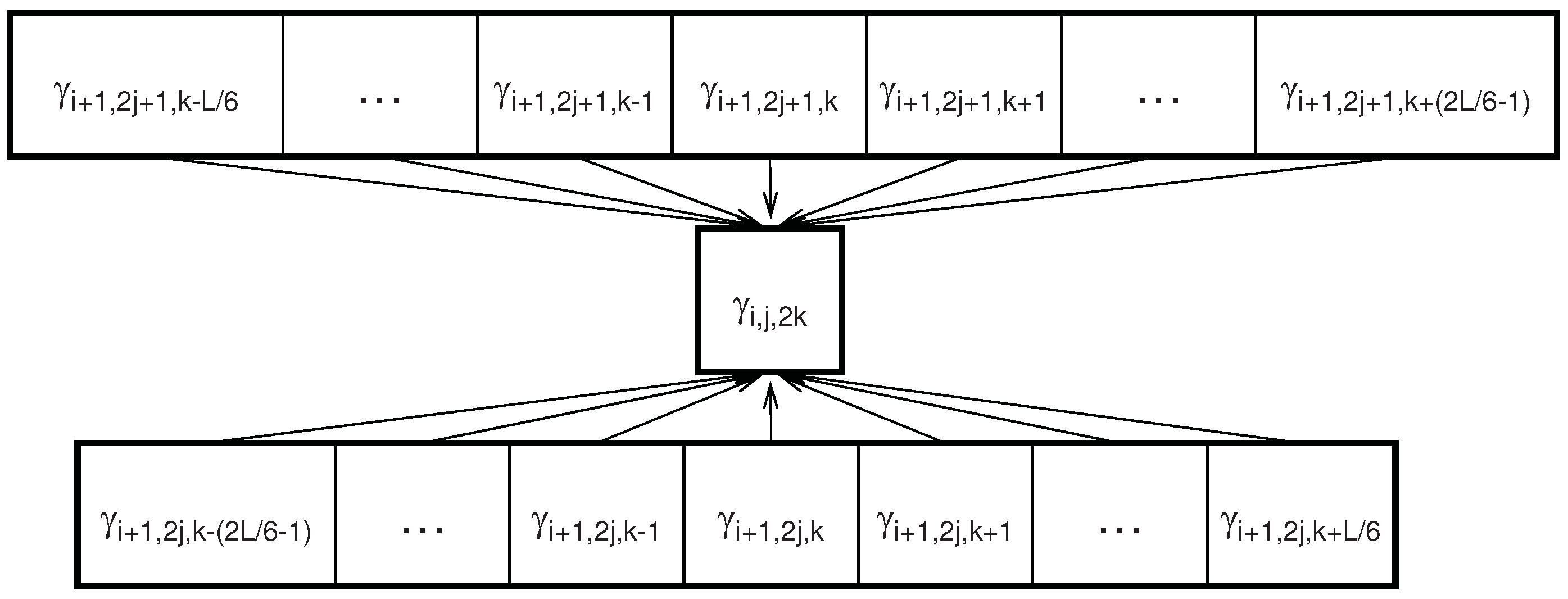
4.1. Parents or Children Nodes are Joint Markov Blankets

Let us denote by F the set of all wavelet features obtained from a wavelet packet decomposition: F $=\{{\Gamma }_{i,j,k}:0\le i\le lo{g}_2\left(N\right),0\le j\le 2^i-1,0\le k\le N/\left(2^i\right)-1\}$.

Proposition 4.1. The level “i” parent coefficients parent${}_i$(${\Gamma }_{i+1,2j,k}$) in Definition 2.1 form a Markov blanket for ${\Gamma }_{i+1,2j,k}$.

Proof. In order to prove that parent${}_i$(${\Gamma }_{i+1,2j,k}$) is a Markov blanket for ${\Gamma }_{i+1,2j,k}$ we have to show:

$$\begin{array}{c}\hfill MI({\Gamma }_{i+1,2j,k};C,\mathbf{F}\setminus \{paren{t}_i\left({\Gamma }_{i+1,2j,k}\right)\cup {\Gamma }_{i+1,2j,k}\}|paren{t}_i\left({\Gamma }_{i+1,2j,k}\right))=0\end{array}$$

(23)

The proof is obtained by expanding the mutual information in its entropy terms:

$$\begin{array}{ccc}& & MI({\Gamma }_{i+1,2j,k};C,\mathbf{F}\setminus \{paren{t}_i\left({\Gamma }_{i+1,2j,k}\right)\cup {\Gamma }_{i+1,2j,k}\}|paren{t}_i\left({\Gamma }_{i+1,2j,k}\right))=\hfill \end{array}$$

$$\begin{array}{ccc}& & H\left({\Gamma }_{i+1,2j,k}\right|paren{t}_i\left({\Gamma }_{i+1,2j,k}\right))\hfill \end{array}$$

$$\begin{array}{ccc}& & -H\left({\Gamma }_{i+1,2j,k}\right|paren{t}_i\left({\Gamma }_{i+1,2j,k}\right),C,\mathbf{F}\setminus \{paren{t}_i\left({\Gamma }_{i+1,2j,k}\right)\cup {\Gamma }_{i+1,2j,k}\})\hfill \end{array}$$

(24)

The first entropy term in Equation (24), $H\left({\Gamma }_{i+1,2j,k}\right|paren{t}_i\left({\Gamma }_{i+1,2j,k}\right))$, is equal to 0. This is due to the fact that ${\Gamma }_{i+1,2j,k}$ is a function of parent${}_i$(${\Gamma }_{i+1,2j,k}$), according to Equation (9) and Definition 2.1. Hence the uncertainty left about ${\Gamma }_{i+1,2j,k}$ after observing parent${}_i$(${\Gamma }_{i+1,2j,k}$) is 0. The second term in Equation (24), $H\left({\Gamma }_{i+1,2j,k}\right|paren{t}_i\left({\Gamma }_{i+1,2j,k}\right),C,\mathbf{F}\setminus \{paren{t}_i\left({\Gamma }_{i+1,2j,k}\right)\cup {\Gamma }_{i+1,2j,k}\})$ must also be equal to 0 for the same reason. From both terms equal to 0 in Equation (24) we can conclude that $MI({\Gamma }_{i+1,2j,k};C,\mathbf{F}\setminus \{paren{t}_i\left({\Gamma }_{i+1,2j,k}\right)\cup {\Gamma }_{i+1,2j,k}\}|paren{t}_i\left({\Gamma }_{i+1,2j,k}\right))=0$ and thus $paren{t}_i\left({\Gamma }_{i+1,2j,k}\right)$ forms a Markov blanket for ${\Gamma }_{i+1,2j,k}$. □

Corollary 4.2. The level “i” parent coefficients parent${}_i$(${\Gamma }_{i+1,2j+1,k}$) form a Markov blanket for ${\Gamma }_{i+1,2j+1,k}$.

The proof occurs in a similar way as in Proposition 4.1.

Corollary 4.3 The level “i+1” child coefficients child${}_{i+1}$(${\Gamma }_{i,j,k}$) in Definition 2.2 form a Markov blanket for ${\Gamma }_{i,j,k}$.

Proof. In order to prove that child${}_{i+1}$(${\Gamma }_{i,j,k}$) is a Markov blanket for ${\Gamma }_{i,j,k}$ we have to show:

$$\begin{array}{c}\hfill MI({\Gamma }_{i,j,k};C,\mathbf{F}\setminus \{chil{d}_{i+1}\left({\Gamma }_{i,j,k}\right)\cup {\Gamma }_{i,j,k}\}|chil{d}_{i+1}\left({\Gamma }_{i,j,k}\right))=0\end{array}$$

(25)

Expansion of the mutual information in entropy terms leads to:

$$\begin{array}{ccc}& & MI({\Gamma }_{i,j,k};C,\mathbf{F}\setminus \{chil{d}_{i+1}\left({\Gamma }_{i,j,k}\right)\cup {\Gamma }_{i,j,k}\}|chil{d}_{i+1}\left({\Gamma }_{i,j,k}\right))=\hfill \end{array}$$

$$\begin{array}{ccc}& & H\left({\Gamma }_{i,j,k}\right|chil{d}_{i+1}\left({\Gamma }_{i,j,k}\right))\hfill \end{array}$$

$$\begin{array}{ccc}& & -H\left({\Gamma }_{i,j,k}\right|chil{d}_{i+1}\left({\Gamma }_{i,j,k}\right),C,\mathbf{F}\setminus \{chil{d}_{i+1}\left({\Gamma }_{i,j,k}\right)\cup {\Gamma }_{i,j,k}\})\hfill \end{array}$$

(26)

Similarly as in the proof of Proposition 4.1 the first entropy term $H\left({\Gamma }_{i,j,k}\right|chil{d}_{i+1}\left({\Gamma }_{i,j,k}\right))=0$ due to functional dependence of ${\Gamma }_{i,j,k}$ on child${}_{i+1}$(${\Gamma }_{i,j,k}$). The second term in Equation (26) is equal to zero for the same reason. □

Using Theorem 3.4 iteratively on all wavelet coefficients in a node we can show that child nodes (or its parent node) form joint Markov blankets.

Proposition 4.4. The set of all wavelet coefficient features in the child nodes ${\left\{{\Gamma }_{i+1,2j,m}\right\}}_{0\le m\le N/\left(2^{i+1}\right)-1}$ and ${\left\{{\Gamma }_{i+1,2j+1,m}\right\}}_{0\le m\le N/\left(2^{i+1}\right)-1}$ form a “joint” Markov blanket for ${\left\{{\Gamma }_{i,j,k}\right\}}_{0\le k\le N/\left(2^i\right)-1}$.

Proof. We can start iterative Markov blanket filtering from any coefficient ${\Gamma }_{i,j,k1}$ in node (i,j) and remove this coefficient based on a Markov blanket child${}_{i+1}$(${\Gamma }_{i,j,k1}$) according to Corollary 4.3. Next we can select a coefficient ${\Gamma }_{i,j,k2}$ in node (i,j) and remove this based on a Markov blanket child${}_{i+1}$(${\Gamma }_{i,j,k2}$). Then according to Theorem 3.4, child${}_{i+1}$(${\Gamma }_{i,j,k1}$) ∪ child${}_{i+1}$(${\Gamma }_{i,j,k2}$) is a joint Markov blanket for ${\Gamma }_{i,j,k1}$ ∪ ${\Gamma }_{i,j,k2}$. We can iterate this over all coefficients in node (i,j): ${\left\{{\Gamma }_{i,j,k}\right\}}_{0\le k\le N/\left(2^i\right)-1}$. Applying Theorem 3.4 iteratively, we find that a joint Markov blanket for all coefficients in node (i,j) is formed by: ${\displaystyle \bigcup _{0\le k\le N/\left(2^i\right)-1}chil{d}_{i+1}\left({\Gamma }_{i,j,k}\right)}$, which is equal to the set of all coefficients of node (i+1,2j): ${\left\{{\Gamma }_{i+1,2j,m}\right\}}_{0\le m\le N/\left(2^{i+1}\right)-1}$ and node (i+1,2j+1): ${\left\{{\Gamma }_{i+1,2j+1,m}\right\}}_{0\le m\le N/\left(2^{i+1}\right)-1}$. This is due to the fact that $chil{d}_{i+1}\left({\Gamma }_{i,j,k}\right)$ coefficients only come from node (i+1,2j) and node (i+1,2j+1) according to Definition 2.2.

Proposition 4.5. The set of all wavelet coefficient features in the parent node ${\left\{{\Gamma }_{i-1,j,m}\right\}}_{0\le m\le N/\left(2^{i-1}\right)-1}$ form a “joint” Markov blanket for ${\left\{{\Gamma }_{i,2j,k}\right\}}_{0\le k\le N/\left(2^i\right)-1}$ and ${\left\{{\Gamma }_{i,2j+1,k}\right\}}_{0\le k\le N/\left(2^i\right)-1}$.

Proof. The proof is similar to Proposition 4.4. Applying Markov blanket filtering iteratively to the coefficients ${\Gamma }_{i,2j,k}$ and ${\Gamma }_{i,2j+1,k}$ in nodes (i,2j) and (i,2j+1) one finds (applying Theorems 3.4, 4.1 and Corollary 4.2 iteratively similar as in Proposition 4.4) that: ${\displaystyle \bigcup _{0\le k\le N/\left(2^i\right)-1}paren{t}_{i-1}\left({\Gamma }_{i,2j,k}\right)\cup paren{t}_{i-1}\left({\Gamma }_{i,2j+1,k}\right)}$ is a joint Markov blanket for all coefficients in nodes (i,2j) and (i,2j+1). This is equal to the set of all coefficients of node (i-1,j): ${\left\{{\Gamma }_{i-1,j,m}\right\}}_{0\le m\le N/\left(2^{i-1}\right)-1}$, because the coefficients $paren{t}_{i-1}\left({\Gamma }_{i,2j,k}\right)$ and $paren{t}_{i-1}\left({\Gamma }_{i,2j+1,k}\right)$ only come from node (i-1,j) according to Definition 2.1. □

Summarizing the results of Propositions 4.4 and 4.5, we see that all coefficients in a node (i,2j) can be removed either by existence of its child nodes (i+1,2.2j) and (i+1,2.2j+1) or by existence of its parent node (i-1,j). Both node (i-1,j) or nodes (i+1,2.2j) and (i+1,2.2j) are guaranteed to form a joint Markov blanket. It is interesting to note that node (i-1,j) contains $N/\left(2^{i-1}\right)$ coefficients and nodes (i+1,2.2j), (i+1,2.2j+1) jointly contain $(N/2^i)$ coefficients which forms a smaller blanket. However, if one selects node (i-1,j) as a joint Markov blanket for removal of (i,2j), it will also be a joint blanket for (i,2j+1).

4.2. Child Nodes are Joint Markov Blankets for Energy Features

Here, the set of all features F consists of all energy features obtained from a wavelet packet decomposition: F $=\{E_i^j:0\le i\le lo{g}_2\left(N\right),0\le j\le 2^i-1\}$.

In case of the energy features, the analysis of dependencies between features is somewhat simpler. As shown in Equation (12), energy features at level “i” (E${}_i^j$) depend functionally on E${}_{i+1}^{2j}$ and E${}_{i+1}^{2j+1}$. Hence, in this case there are only child features that determine level “i” features. This leads to Corollary 4.6 (similar to Corollary 4.3).

Corollary 4.6. Energy features E${}_{i+1}^{2j}$ and E${}_{i+1}^{2j+1}$ form a Markov blanket for E${}_i^j$.

Proof. In order for E${}_{i+1}^{2j}$ and E${}_{i+1}^{2j+1}$ to form a Markov blanket for E${}_i^j$, it needs to be shown that: $MI(E_i^j;C,\mathbf{F}\setminus \{E_i^j\cup E_{i+1}^{2j}\cup E_{i+1}^{2j+1}\}|E_{i+1}^{2j}\cup E_{i+1}^{2j+1})=0$. Using the expansion of the mutual information in its entropy terms yields:

$$\begin{array}{ccc}& & MI(E_i^j;C,\mathbf{F}\setminus \{E_i^j\cup E_{i+1}^{2j}\cup E_{i+1}^{2j+1}\}|E_{i+1}^{2j}\cup E_{i+1}^{2j+1})=\hfill \end{array}$$

$$\begin{array}{ccc}& & H\left(E_i^j\right|E_{i+1}^{2j}\cup E_{i+1}^{2j+1})-H\left(E_i^j\right|\{E_{i+1}^{2j}\cup E_{i+1}^{2j+1}\},C,\mathbf{F}\setminus \{E_i^j\cup E_{i+1}^{2j}\cup E_{i+1}^{2j+1}\})\hfill \end{array}$$

(27)

The first term in Equation (27) $H\left(E_i^j\right|E_{i+1}^{2j}\cup E_{i+1}^{2j+1})$ is equal to 0 due to functional dependence, the second term is equal to 0 for the same reason (see also the proof of Proposition 4.1).□

For the set of energy features, we obtain following result on which energy features form a “joint” Markov blanket for all other energy features.

Proposition 4.7. The highest frequency energy features ${\left\{E_{lo{g}_2\left(N\right)}^j\right\}}_{0\le j\le N-1}$ form a joint Markov blanket for all other energy features F $\setminus {\left\{E_{lo{g}_2\left(N\right)}^j\right\}}_{0\le j\le N-1}$.

Proof. Iterative elimination of features based on Markov blankets starting from the top of a wavelet tree (as in Figure 2) proceeds as follows. Starting from the top, feature E${}_0^0$ can be removed because E${}_1^0$∪ E${}_1^1$ forms a Markov blanket according to Corollary 4.6. Next, E${}_1^0$ can be removed because E${}_2^0$∪ E${}_2^1$ forms a Markov blanket according to Corollary 4.6. Using Theorem 3.4, E${}_2^0$∪ E${}_2^1$ ∪ E${}_1^1$ forms a joint Markov blanket for E${}_0^0$ ∪ E${}_1^0$. Next E${}_1^1$ can be removed based on E${}_2^2$ and E${}_2^3$. We then obtain that E${}_2^0$∪ E${}_2^1$ ∪ E${}_2^2$ ∪ E${}_2^3$ is a joint blanket for E${}_0^0$ ∪ E${}_1^0$ ∪ E${}_1^1$. Hence, iterating this procedure until arriving at ${\left\{E_{lo{g}_2\left(N\right)}^j\right\}}_{0\le j\le N-1}$, these features form a joint blanket for: ${\left\{E_i^j\right\}}_{0\le i\le lo{g}_2\left(N\right)-1,0\le j\le 2^i-1}$ = F$\setminus {\left\{E_{lo{g}_2\left(N\right)}^j\right\}}_{0\le j\le N-1}$. □

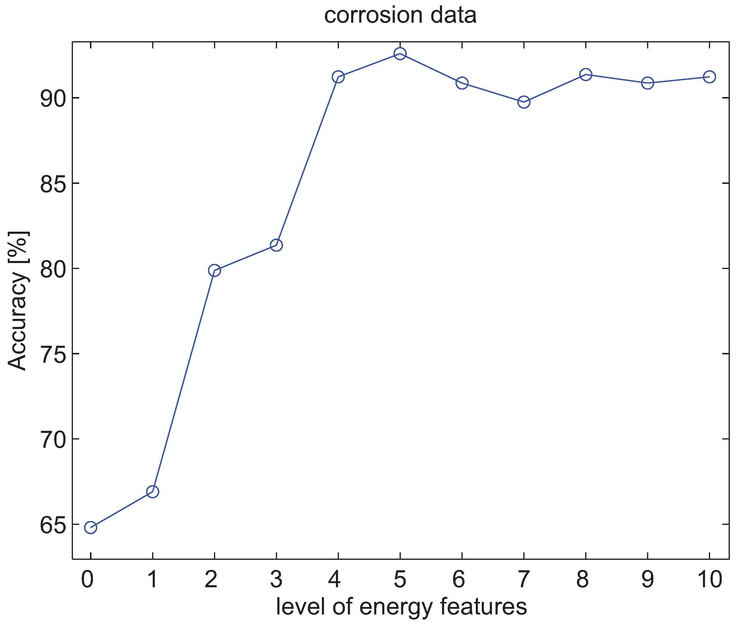
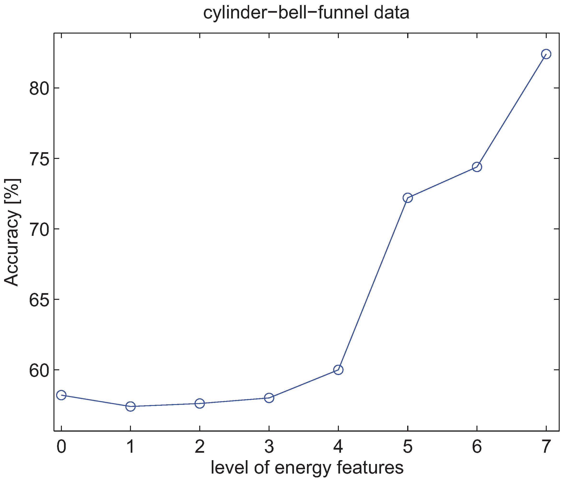
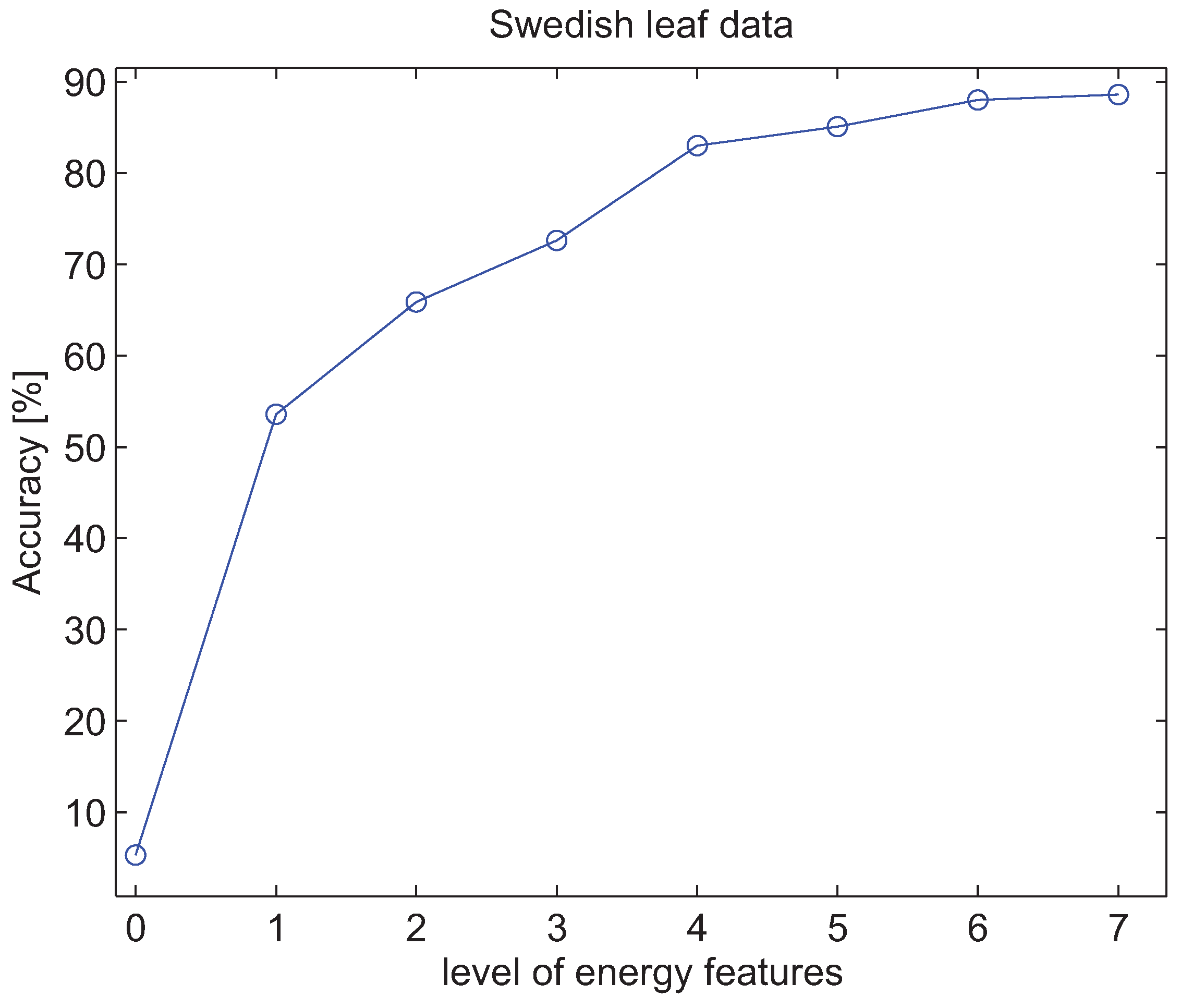
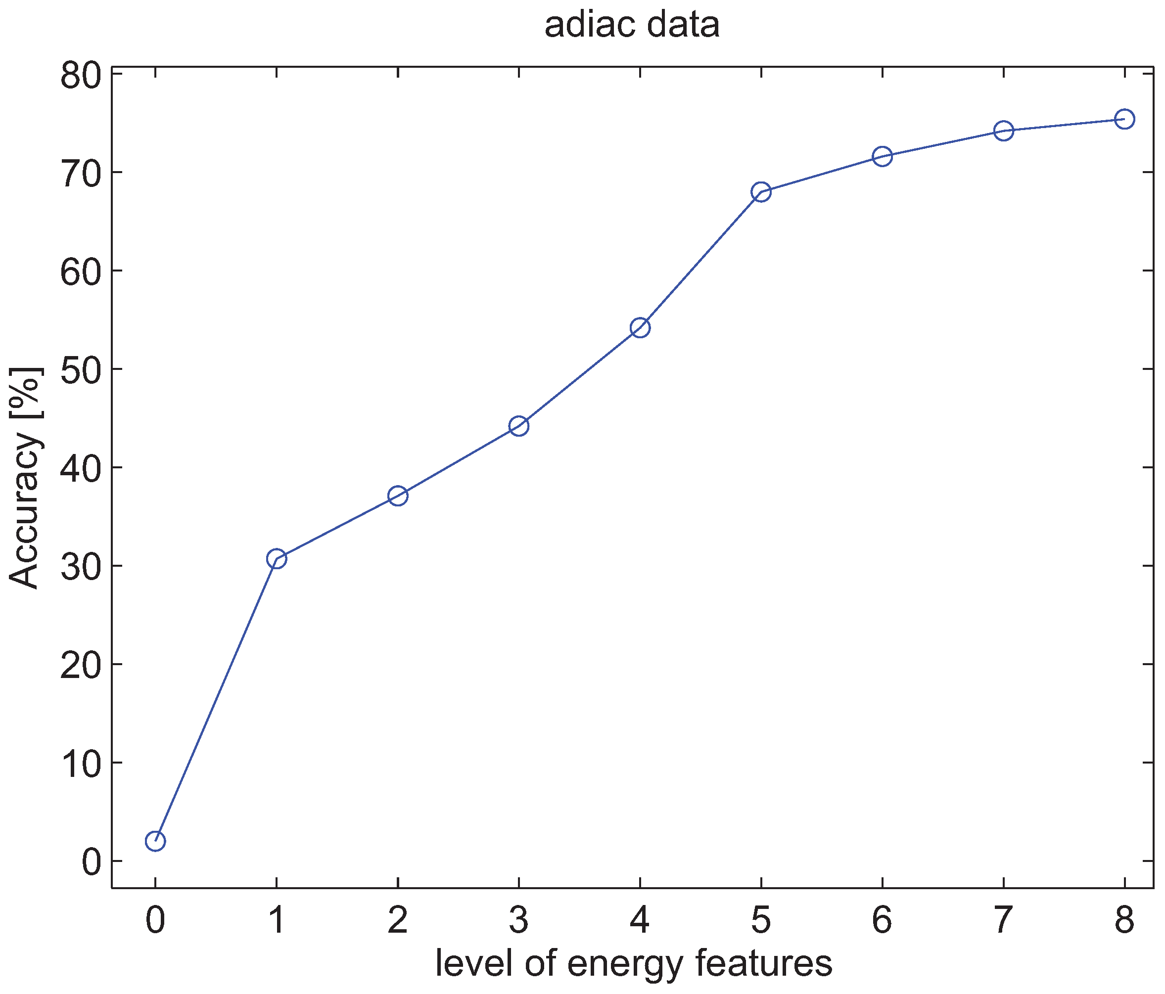
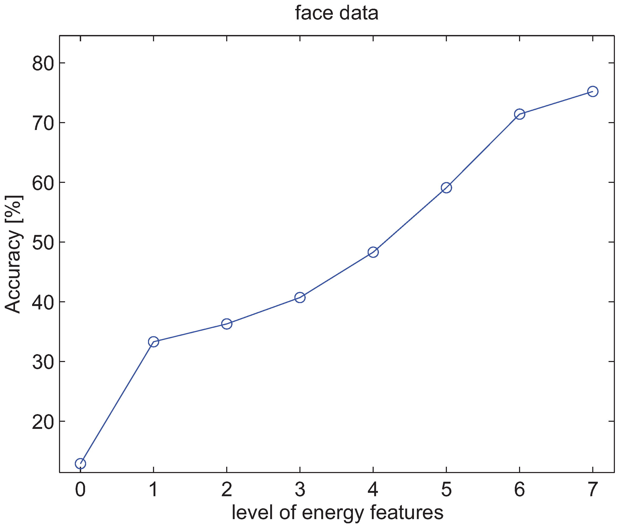
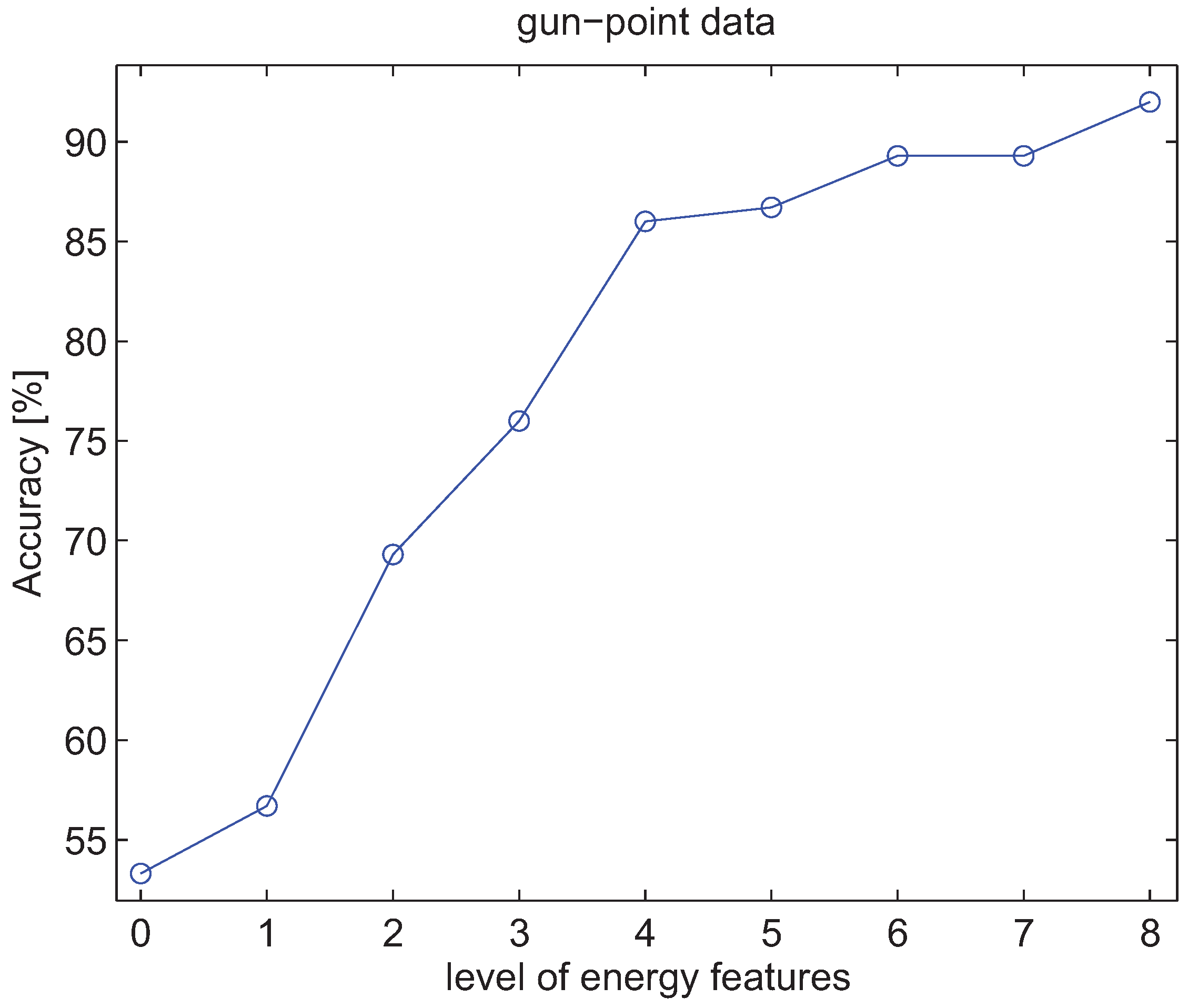
4.3. Experiments with Energy Features of Wavelet Packet Decomposition

As shown in the proof of Proposition 4.7, energy features at level i+1, i.e., E${}_{i+1}^0$, ... E${}_{i+1}^{2^{i+1}-1}$, form a joint Markov blanket for the features at level i (as well as for those at levels i-1, ... 0). This implies that the set {E${}_i^0$, ... E${}_i^{2^i-1}$} contains no information about the target variable “C” that is not covered yet by the set {E${}_{i+1}^0$, ... E${}_{i+1}^{2^{i+1}-1}$}. The latter implies that $MI(\{E_i^0,...E_i^{2^i-1}\};C)$≤ $MI(\{E_{i+1}^0,...E_{i+1}^{2^{i+1}-1}\};C)$. Furthermore, we know there is a close relationship between the mutual information and the probability of error (Pe) for predicting a target variable [30]. In particular, the Kovalevsky upper bound [39] is known to be a tight upper bound [40] on the probability of error as a function of the mutual information. With increasing mutual information the upper bound on the probability of error becomes smaller and smaller, see, e.g., [30]. The consequence is that the probability of error is expected to decrease with increasing level of the energy features. This behavior may be observed from an increasing testing accuracy when a classifier is trained with energy features of increasing levels. However, this behavior can be expected only at the lower levels: 0, 1, 2, 3, ... Indeed the number of energy features at level “i” increases as $2^i$ and hence the curse of dimensionality [41] may become dominant at higher levels which implies that the testing performance decreases again. This behavior is dependent on the particular classifier being used as well as on the ratio of the number of training patterns “N” to the dimensionality “d” of the patterns: N/d [42,43,44]. Next, we will illustrate the increasing classification accuracy with increasing level of the energy features as expected from the joint Markov blankets explained in previous paragraph. We consider six different time series classification problems. The corrosion data set consists of 4 classes: absence of corrosion (197 signals), uniform corrosion (194 signals), pitting (214 signals) and stress corrosion cracking (205 signals). The signals are acoustic emission signals that were obtained during each of the corrosion processes. A trained classifier can be used to predict which corrosion process is active based on the emitted acoustic signals. For a background on the origin of the acoustic activity and the details of the experiments, the reader is referred to [9,10]. We applied the C-SVC (C-Support Vector Classifier) [45] using the LIBSVM software [46]. For more background information on SVM’s (Support Vector Machine) see, e.g., [47,48,49,50]. We used a linear kernel and a grid search within the training set, see also [46], to find the best cost parameter C. In the grid search, we performed a 5-fold cross-validation and varied the cost parameter from C = 2${}^{-5}$, 2${}^{-4}$, ... 2${}^{15}$. The testing accuracy was obtained by means of a 10-fold cross-validation. We used the 12-tap Coiflet filter to compute the energy features. The same settings were used for the other time series classification problems, unless mentioned otherwise, with the exception that we dispose of separate training and test sets. The evolution of the testing accuracy as a function of the level of the energy features is shown in Figure 6. As predicted from the joint Markov blanket theory, at the lower levels the classification accuracy is expected to increase, but starting at level 6 (with 2${}^6$ energy features) the classification accuracy starts to fluctuate which can be partly attributed to the curse of dimensionality. In order to deal with the curse of dimensionality, one could further apply a feature subset selection algorithm to the energy features extracted from the highest frequency resolution.

Figure 6. Evolution of the classification accuracy as a function of the level of the energy features for the corrosion data set.

Figure 6. Evolution of the classification accuracy as a function of the level of the energy features for the corrosion data set.

The second time series classification problem is the cylinder-bell-funnel class problem defined by Saito and Coifman [6]. The cylinder, bell and funnel class are defined respectively as [6]:

$$\begin{array}{ccc}& & c\left(i\right)=(6+\eta ).{\chi }_{[a,b]}.\left(i\right)+ϵ\left(i\right)\text{for cylinder class}\hfill \end{array}$$

(28)

$$\begin{array}{ccc}& & b\left(i\right)=(6+\eta ).{\chi }_{[a,b]}.(i-a)/(b-a)+ϵ\left(i\right)\text{for bell class}\hfill \end{array}$$

(29)

$$\begin{array}{ccc}& & f\left(i\right)=(6+\eta ).{\chi }_{[a,b]}.(b-i)/(b-a)+ϵ\left(i\right)\text{for funnel class}\hfill \end{array}$$

(30)

where i = 1,...128, a is an integer-valued uniform random variable in the interval [16, 32], similarly (b-a) follows an integer-valued uniform distribution on the interval [32, 96], η and $ϵ\left(i\right)$ are standard normal random variables and ${\chi }_{[a,b]}$ is the characteristic function on the interval [a, b]. We generated 100 training times series for each class and 1000 testing time series for each class. The tendency of increasing performance with increasing level of energy features is largely confirmed in Figure 7.

The face (all) data set consists of 14 different subjects (classes) with 560 training examples and 1690 testing examples. There are 131 time series points for each subject; we restricted this to the first 128 time series points in order to have a power of two number of samples before applying the WPD. The increasing performance with increasing energy levels is confirmed in Figure 8. Note that the performance (75.2%) at the highest energy level (7) is higher than obtained with the 1-NN Euclidean distance classifier (71.4%, see [51]), but lower than obtained with time warping (80.2%) reported in [51]. This is a typical data set to test time warping algorithms.

Figure 7. Evolution of the classification accuracy as a function of the level of the energy features for the cylinder-bell-funnel data set.

Figure 7. Evolution of the classification accuracy as a function of the level of the energy features for the cylinder-bell-funnel data set.

Figure 8. Evolution of the classification accuracy as a function of the level of the energy features for the face data set. Training and testing data set are available [51].

Figure 8. Evolution of the classification accuracy as a function of the level of the energy features for the face data set. Training and testing data set are available [51].

The gun-point data set consists of 2 classes, with 50 time series in the training set and 150 time series in the testing set [51]. The time series count 150 samples, these have been zero-padded to 256 samples before applying the WPD. We used the radial basis function (RBF) kernel in the SVM. In the grid search, we performed a 5-fold cross-validation in which we varied the cost parameter from C = 2${}^{-5}$, 2${}^{-4}$, ... 2${}^{15}$ and varied the kernel parameter from γ = 2${}^{-15}$, 2${}^{-14}$, ... 2${}^3$. At the highest energy level we achieved a performance of 92.0%, see Figure 9, which is higher than obtained with the 1-NN Euclidean distance classifier (91.3%) and than obtained with time warping (91.3%) [51].

Figure 9. Evolution of the classification accuracy as a function of the level of the energy features for the gun-point data set. Training and testing data set are available [51].

Figure 9. Evolution of the classification accuracy as a function of the level of the energy features for the gun-point data set. Training and testing data set are available [51].

The Swedish leaf data set consists of 15 classes and contains 500 time series in the training set and 625 time series in the testing set. Figure 10 shows the increasing classification accuracy with increasing energy levels. The performance at level 8, 88.6%, is higher than the 78.7% for the 1-NN Euclidean distance classifier and higher than for time warping 84.3% reported in [51].

Figure 10. Evolution of the classification accuracy as a function of the level of the energy features for the Swedish leaf data set. Training and testing data set are available [51].

Figure 10. Evolution of the classification accuracy as a function of the level of the energy features for the Swedish leaf data set. Training and testing data set are available [51].

The adiac data set consists of 37 classes, 390 training time series and 391 testing time series [51]. The time series contain 176 samples and these have been zero-padded to 256 samples before applying the WPD. The increasing accuracy with increasing energy levels is again confirmed as supported by the joint Markov blanket theory. The result obtained at level 8 (75.4%) in Figure 11 is higher than obtained with the 1-NN Euclidean distance classifier (61.1%) and time warping (60.9%) [51].

Figure 11. Evolution of the classification accuracy as a function of the level of the energy features for the adiac data set. Training and testing data set are available [51].

Figure 11. Evolution of the classification accuracy as a function of the level of the energy features for the adiac data set. Training and testing data set are available [51].

5. Conclusions

We have argued that within feature subset selection research, wavelet packet decompositions need special attention due to the existence of many dependencies between features. We extended Markov blanket filtering to the theory of joint Markov blankets in Theorem 3.4 by exploiting the link between the information-theoretic mutual information selection criterion and Markov blanket filtering. Analytical results on the existence of joint Markov blankets were established in some propositions.

It was shown that joint Markov blankets exist for both the wavelet coefficient features and the energy features, regardless of the underlying distribution within signals and images. In case of wavelet coefficient features, it was proven in Proposition 4.4 that all wavelet coefficient features in the child nodes ${\left\{{\Gamma }_{i+1,2j,m}\right\}}_{0\le m\le N/\left(2^{i+1}\right)-1}$ and ${\left\{{\Gamma }_{i+1,2j+1,m}\right\}}_{0\le m\le N/\left(2^{i+1}\right)-1}$ of ${\left\{{\Gamma }_{i,j,k}\right\}}_{0\le k\le N/\left(2^i\right)-1}$ form a joint Markov blanket. In Proposition 4.5 it was shown that the parent node ${\left\{{\Gamma }_{i-1,j,m}\right\}}_{0\le m\le N/\left(2^{i-1}\right)-1}$ forms a joint Markov blanket for ${\left\{{\Gamma }_{i,2j,k}\right\}}_{0\le k\le N/\left(2^i\right)-1}$ and ${\left\{{\Gamma }_{i,2j+1,k}\right\}}_{0\le k\le N/\left(2^i\right)-1}$.

For the energy features it was proven in Proposition 4.7 that the highest resolution features ${\left\{E_{lo{g}_2\left(N\right)}^j\right\}}_{0\le j\le N-1}$ form a joint Markov blanket for all other energy features. In six experiments it was confirmed that with increasing level of energy features the classification accuracy is expected to increase as explained by the joint Markov blanket theory. However, this behavior is observed only for the lower levels in the corrosion data set. At higher levels, the curse of dimensionality may reduce the classification accuracy due to the increasing number of energy features.

References

1. Coifman, R.R.; Meyer, Y. Orthonormal wave packet bases; Technical report; Yale University, 1990. [Google Scholar]
2. Mallat, S. A theory for multiresolution signal decomposition: The wavelet decomposition. IEEE Trans. Pattern Anal. Mach. Intell. 1989, 11, 674–693. [Google Scholar] [CrossRef]
3. Mallat, S. A Wavelet Tour of Signal Processing; Academic Press: New York, NY, USA, 1998. [Google Scholar]
4. Wickerhauser, M.V. INRIA lectures on wavelet packet algorithms. In Proceedings of Ondelettes et Paquets d’Ondes; 17–21 June 1991; Lions, P.L., Ed.; INRIA: Rocquencourt, France; pp. 31–99.
5. Coifman, R.R.; Wickerhauser, M.V. Entropy-based algorithm for best basis selection. IEEE Trans. Inf. Theory 1992, 38, 713–718. [Google Scholar] [CrossRef]
6. Saito, N.; Coifman, R.R. Local discriminant bases and their applications. J. Math. Imaging Vis. 1995, 5, 337–358. [Google Scholar] [CrossRef]
7. Saito, N.; Coifman, R.R. Geological information extraction from acoustic well-logging waveforms using time-frequency wavelets. Geophysics 1997, 62, 1921–1930. [Google Scholar] [CrossRef]
8. Saito, N.; Coifman, R.R.; Geshwind, F.B.; Warner, F. Discriminant feature extraction using empirical probability density estimation and a local basis library. Pattern Recogn. 2002, 35, 2481–2852. [Google Scholar] [CrossRef]
9. Van Dijck, G.; Van Hulle, M.M. Wavelet packet decomposition for the identification of corrosion type from acoustic emission signals. Int. J. Wavelets Multiresolut. Inf. Process. 2009, 7, 513–534. [Google Scholar] [CrossRef]
10. Van Dijck, G.; Van Hulle, M.M. Information theoretic filters for wavelet packet coefficient selection with application to corrosion type identification from acoustic emission signals. Sensors 2011, 11, 5695–5715. [Google Scholar] [CrossRef] [PubMed]
11. Van Dijck, G. Information Theoretic Approach to Feature Selection and Redundancy Assessment. PhD dissertation, Katholieke Universiteit Leuven, Leuven, Belgium, 2008. [Google Scholar]
12. Huang, K.; Aviyente, S. Information-theoretic wavelet packet subband selection for texture classification. Signal Process. 2006, 86, 1410–1420. [Google Scholar] [CrossRef]
13. Huang, K.; Aviyente, S. Wavelet feature selection for image classification. IEEE Trans. Image Process. 2008, 17, 1709–1720. [Google Scholar] [CrossRef] [PubMed]
14. Laine, A.; Fan, J. Texture classification by wavelet packet signatures. IEEE Trans. Pattern Anal. Mach. Intell. 1993, 15, 1186–1191. [Google Scholar] [CrossRef]
15. Khandoker, A.H.; Palaniswami, M.; Karmakar, C.K. Support vector machines for automated recognition of obstructive sleep apnea syndrome from ECG recordings. IEEE Trans. Inf. Technol. Biomed. 2009, 13, 37–48. [Google Scholar] [CrossRef] [PubMed]
16. Daubechies, I. Ten Lectures on Wavelets; SIAM: Philadelphia, PA, USA, 1992. [Google Scholar]
17. Tewfik, A.H.; Kim, M. Correlation structure of the discrete wavelet coefficients of fractional Brownian motion. IEEE Trans. Inf. Theory 1992, 38, 904–909. [Google Scholar] [CrossRef]
18. Dijkerman, R.W.; Mazumdar, R.R. On the correlation structure of the wavelet coefficients of fractional Brownian motion. IEEE Trans. Inf. Theory 1994, 40, 1609–1612. [Google Scholar] [CrossRef]
19. Koller, D.; Sahami, M. Toward optimal feature selection. In Proceedings of the Thirteenth International Conference on Machine Learning, Bari, Italy, 3–6 July 1996; pp. 284–292.
20. Xing, E.P.; Jordan, M.I.; Karp, M.I. Feature selection for high-dimensional genomic microarray data. In Proceedings of the Eighteenth International Conference on Machine Learning, Williamstown, MA, USA, 28 June–1 July 2001; pp. 601–608.
21. Yu, L.; Liu, H. Efficient feature selection via analysis of relevance and redundancy. J. Mach. Learn. Res. 2004, 5, 1205–1224. [Google Scholar]
22. Nilsson, R.; Peña, J.M.; Björkegren, J.; Tegnér, J. Consistent feature selection for pattern recognition in polynomial time. J. Mach. Learn. Res. 2007, 8, 589–612. [Google Scholar]
23. Peña, J.M.; Nilsson, R.; Björkegren, J.; Tegnér, J. Towards scalable and data efficient learning of Markov boundaries. Int. J. Approx. Reasoning 2007, 45, 211–232. [Google Scholar] [CrossRef]
24. Aliferis, C.F.; Statnikov, A.; Tsamardinos, I.; Mani, S.; Koutsoukos, X.D. Local causal and Markov blanket induction for causal discovery and feature selection for classification part I: Algorithms and empirical evaluation. J. Mach. Learn. Res. 2010, 11, 171–234. [Google Scholar]
25. Rodrigues de Morais, S.; Aussem, A. A novel Markov boundary based feature subset selection algorithm. Neurocomputing 2010, 73, 578–584. [Google Scholar] [CrossRef]
26. Battiti, R. Using mutual information for selecting features in supervised neural net learning. IEEE Trans. Neural Netw. 1994, 5, 537–550. [Google Scholar] [CrossRef] [PubMed]
27. Kwak, N.; Choi, C.H. Input feature selection for classification problems. IEEE Trans. Neural Netw. 2002, 13, 143–159. [Google Scholar] [CrossRef] [PubMed]
28. Kwak, N.; Choi, C.H. Input feature selection by mutual information based on Parzen window. IEEE Trans. Pattern Anal. Mach. Intell. 2002, 24, 1667–1671. [Google Scholar] [CrossRef]
29. Peng, H.; Long, F.; Ding, C. Feature selection based on mutual information: criteria of max-dependency, max-relevance and min-redundancy. IEEE Trans. Pattern Anal. Mach. Intell. 2005, 27, 1226–1238. [Google Scholar] [CrossRef] [PubMed]
30. Van Dijck, G.; Van Hulle, M.M. Increasing and decreasing returns and losses in mutual information feature subset selection. Entropy 2010, 12, 2144–2170. [Google Scholar] [CrossRef]
31. Van Dijck, G.; Van Hulle, M.M. Speeding up feature subset selection through mutual information relevance filtering. In Knowledge Discovery in Databases: PKDD 2007, Proceedings of the 11th European Conference on Principles and Practice of Knowledge Discovery in Databases, Warsaw, Poland, 17–21, September 2007; Kok, J., Koronacki, J., Lopez de Mantaras, R., Matwin, S., Mladenic, D., Skowron, A., Eds.; Springer: Berlin, Heidelberg, Germany, 2007. [Google Scholar]Lect. Notes Comput. Sci. 2007, 4702, 277–287.
32. Van Dijck, G.; Van Hulle, M.M. Speeding up the wrapper feature subset selection in regression by mutual information relevance and redundancy analysis. In Artificial Neural Networks: ICANN 2006, Proceedings of the 16th International Conference on Artificial Neural Networks, Athens, Greece, 10–14 September 2006; Kollias, S.D., Stafylopatis, A., Duch, W., Oja, E., Eds.; Springer: Berlin, Heidelberg, Germany, 2006. [Google Scholar]Lect. Notes Comput. Sci. 2006, 4131, 31–40.
33. Lewis II, P.M. The characteristic selection problem in recognition systems. IEEE Trans. Inf. Theory 1962, 8, 171–178. [Google Scholar] [CrossRef]
34. Meyer, P.; Schretter, C.; Bontempi, G. Information-theoretic feature selection in micro-array data using variable complementarity. IEEE J. Sel. Top. Sign. Proces. 2008, 2, 261–274. [Google Scholar] [CrossRef]
35. John, G.H.; Kohavi, R.; Pfleger, H. Irrelevant feature and the subset selection problem. In Proceedings of the Eleventh International Conference on Machine Learning, New Brunswick, NJ, USA, 10–13 July 1994; pp. 121–129.
36. Cover, T.M.; Thomas, J.A. Elements of Information Theory, 2nd ed.; John Wiley & Sons: Hoboken, NJ, USA, 2006. [Google Scholar]
37. Zheng, Y.; Kwoh, C.K. A feature subset selection method based on high-dimensional mutual information. Entropy 2011, 13, 860–901. [Google Scholar] [CrossRef]
38. Knijnenburg, T.A.; Reinders, M.J.T.; Wessels, L.F.A. Artifacts of Markov blanket filtering based on discretized features in small sample size applications. Pattern Recognit. Lett. 2006, 27, 709–714. [Google Scholar] [CrossRef]
39. Kovalevsky, V.A. The problem of character recognition from the point of view of mathematical statistics. In Character Readers and Pattern Recognition; Kovalevsky, V.A., Ed.; Spartan: New York, NY, USA, 1968. [Google Scholar]
40. Feder, M.; Merhav, N. Relations between entropy and error probability. IEEE Trans. Inf. Theory 1994, 40, 259–266. [Google Scholar] [CrossRef]
41. Duda, R.O.; Hart, P.E.; Stork, D.G. Pattern Classification, 2nd ed.; John Wiley & Sons: New York, NY, USA, 2001. [Google Scholar]
42. Raudys, S.; Jain, A. Small sample size effects in statistical pattern recognition: Recommendations for practitioners. IEEE Trans. Pattern Anal. Mach. Intell. 1991, 13, 252–264. [Google Scholar] [CrossRef]
43. Raudys, S. On dimensionality, sample size and classification error of nonparametric linear classification algorithms. IEEE Trans. Pattern Anal. Mach. Intell. 1997, 19, 667–671. [Google Scholar] [CrossRef]
44. Raudys, S. Statistical and Neural Classifiers: An Integrated Approach to Design; Springer-Verlag: London, UK, 2001. [Google Scholar]
45. Cortes, C.; Vapnik, V. Support-vector network. Mach. Learn. 1995, 20, 273–297. [Google Scholar] [CrossRef]
46. Chang, C.C.; Lin, C.J. LIBSVM: A library for support vector machines. 2001. Software available online: http://www.csie.ntu.edu.tw∼cjlin/libsvm (accessed on 18 July 2011).
47. Kecman, V. Learning and Soft Computing, Support Vector Machines, Neural Networks and Fuzzy Logic Models; The MIT Press: Cambridge, MA, USA, 2001. [Google Scholar]
48. Support Vector Machines: Theory and Application; Wang, L.P. (Ed.) Springer: Berlin, Germany, 2005.
49. Sloin, A.; Burshtein, D. Support vector machine training for improved hidden markov modeling. IEEE Trans. Signal Process. 2008, 56, 172–188. [Google Scholar] [CrossRef]
50. Wang, L.P.; Fu, X.J. Data Mining with Computational Intelligence; Springer: Berlin, Germany, 2005. [Google Scholar]
51. Keogh, E. UCR time series classification/clustering page. Training and testing data sets: Available online: http://www.cs.ucr.edu/ eamonn/time_series_data/ (accessed on 18 July 2011).