Size of the Whole versus Number of Parts in Genomes


Abstract
:
1. Introduction
2. Results
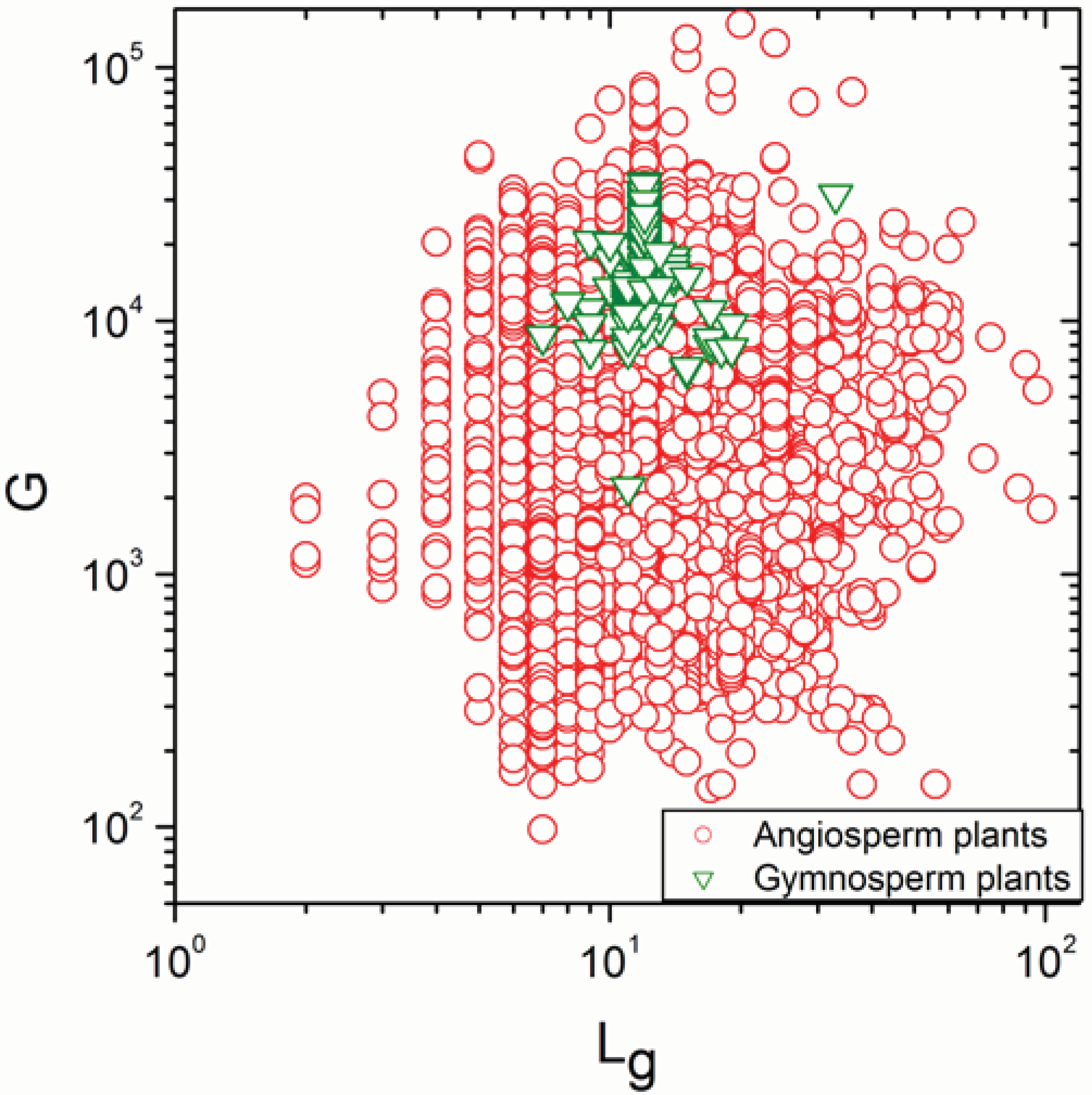
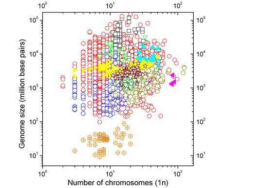
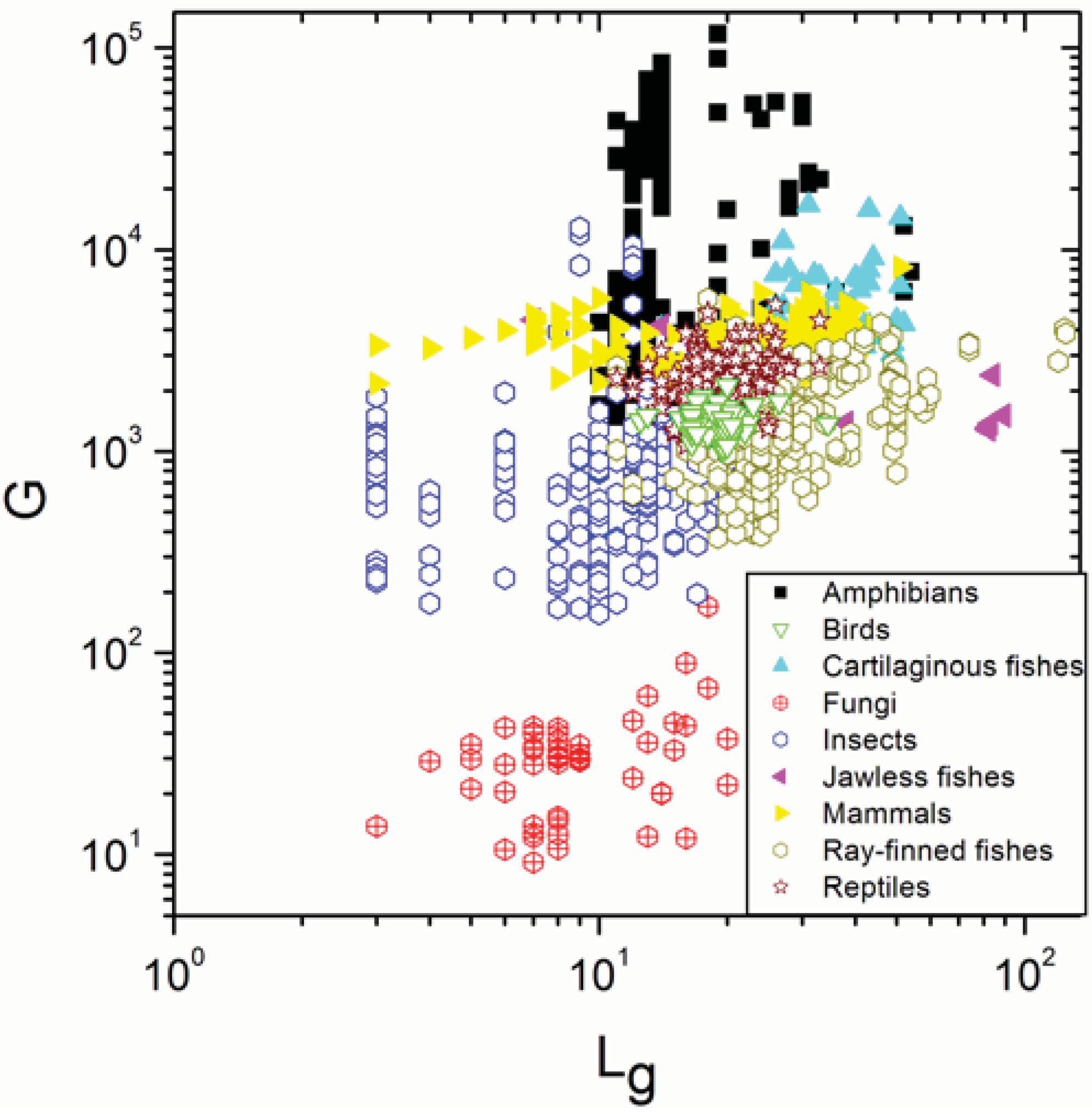
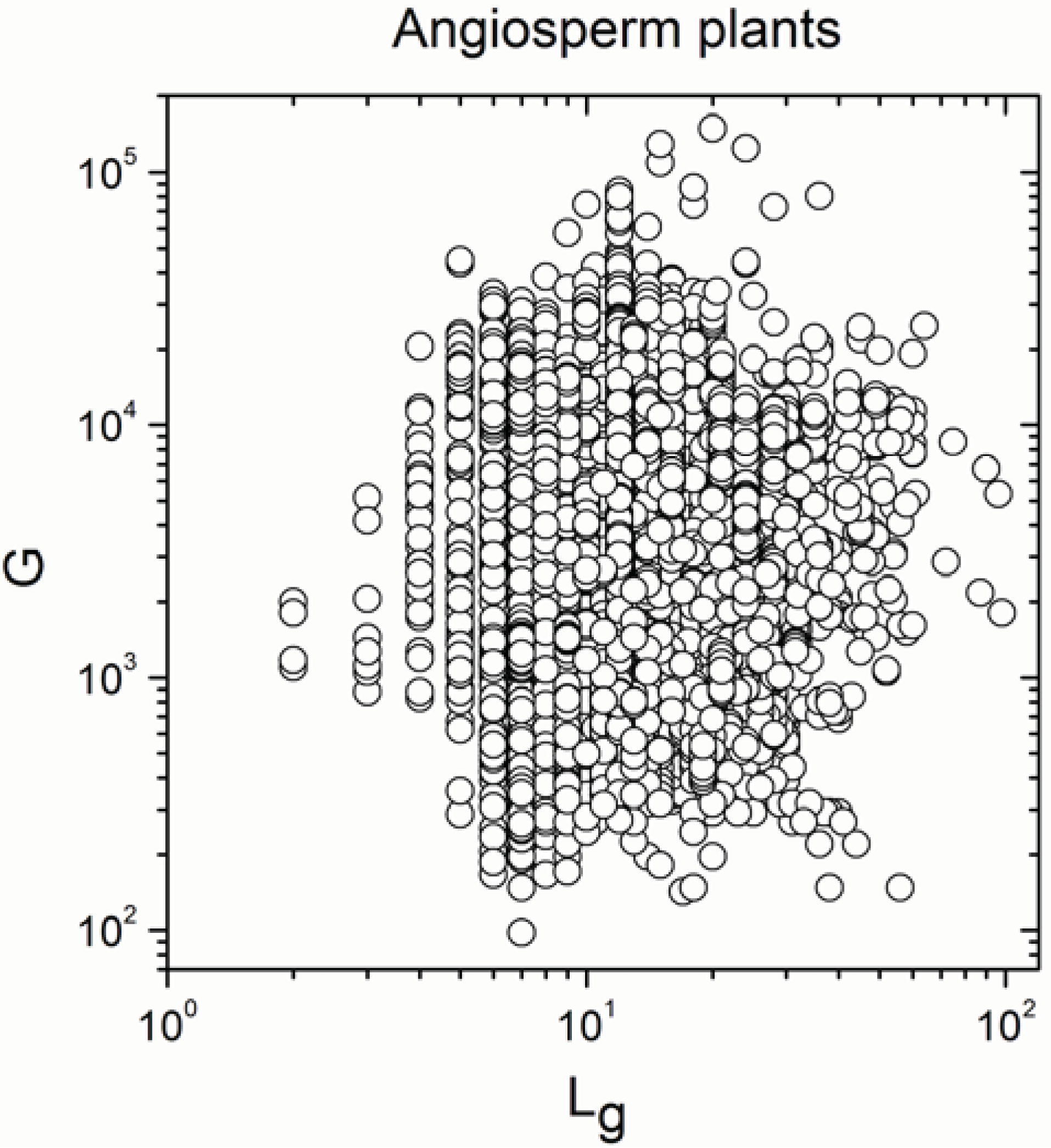
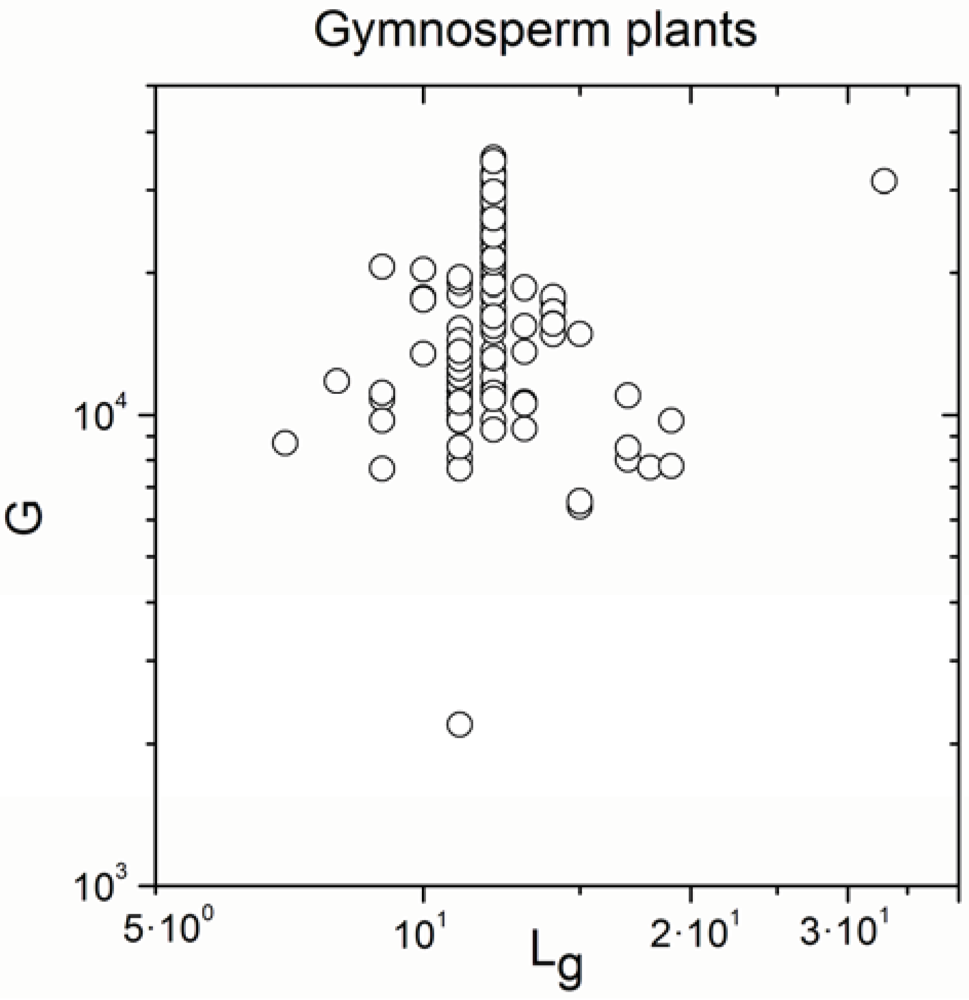
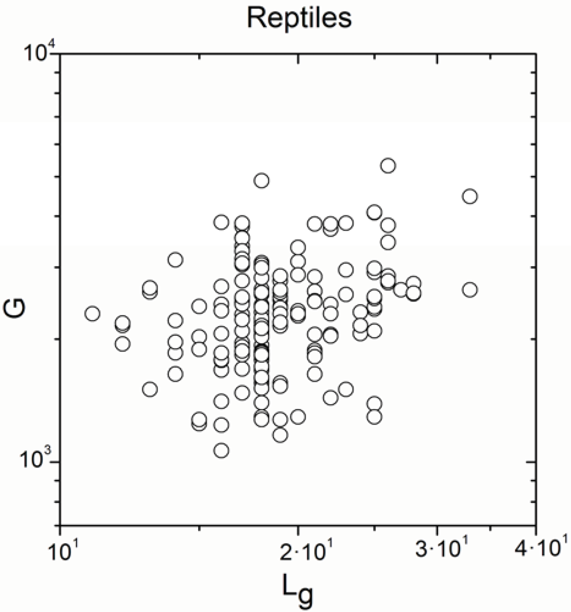
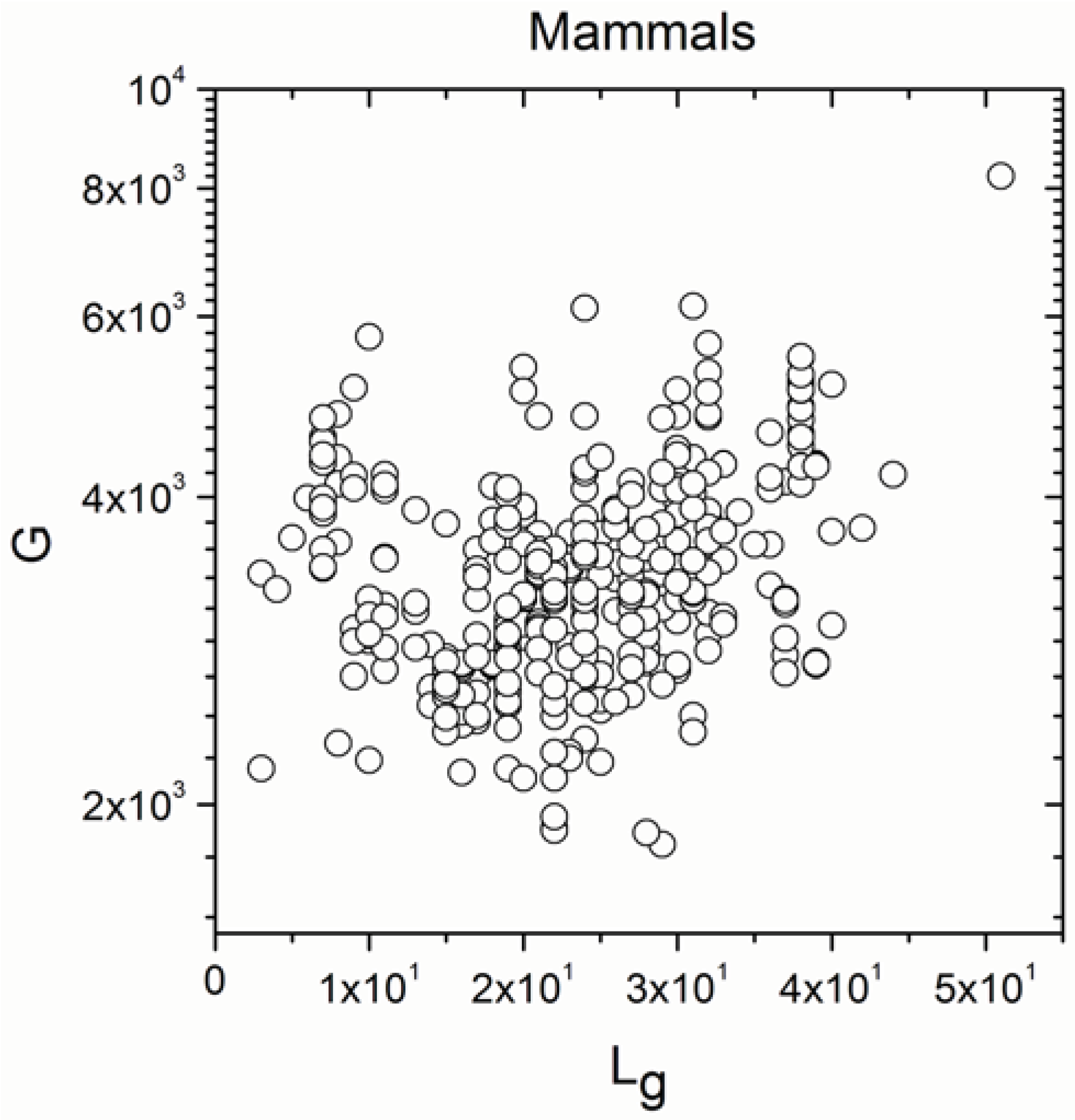
2.1. Correlations between Genome Size and Chromosome Number
2.2. Non-Linearity


| Group | N | ρ | p |
|---|---|---|---|
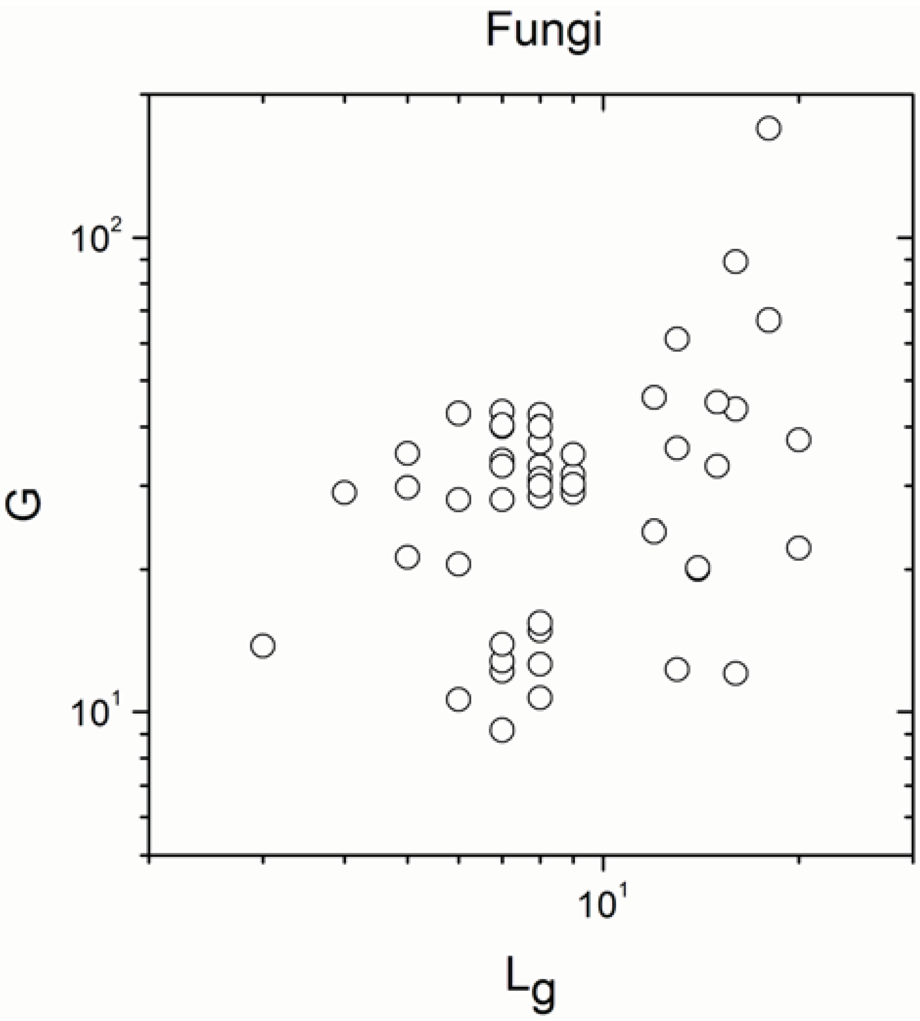
| Fungi | 56 | 0.280 | 0.04 |
| Angiosperm plants | 4706 | −0.38 | 0.008 |
| Gymnosperm plants | 170 | 0.315 | 3 × 10⁻⁵ |
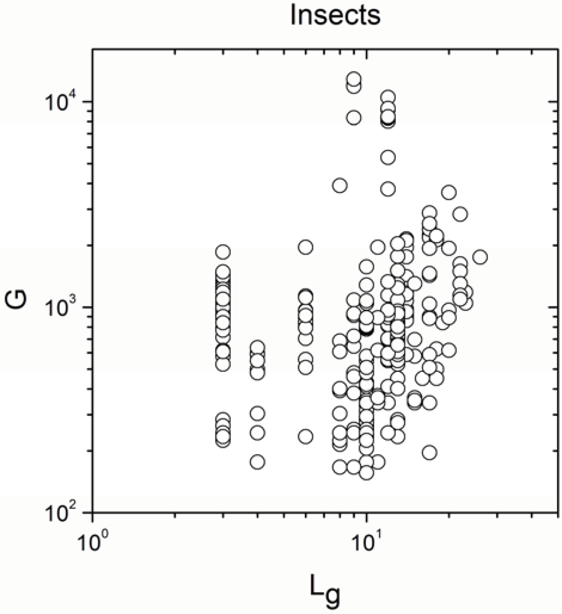
| Insects | 269 | 0.220 | 0.0003 |
| Reptiles | 170 | 0.243 | 0.001 |
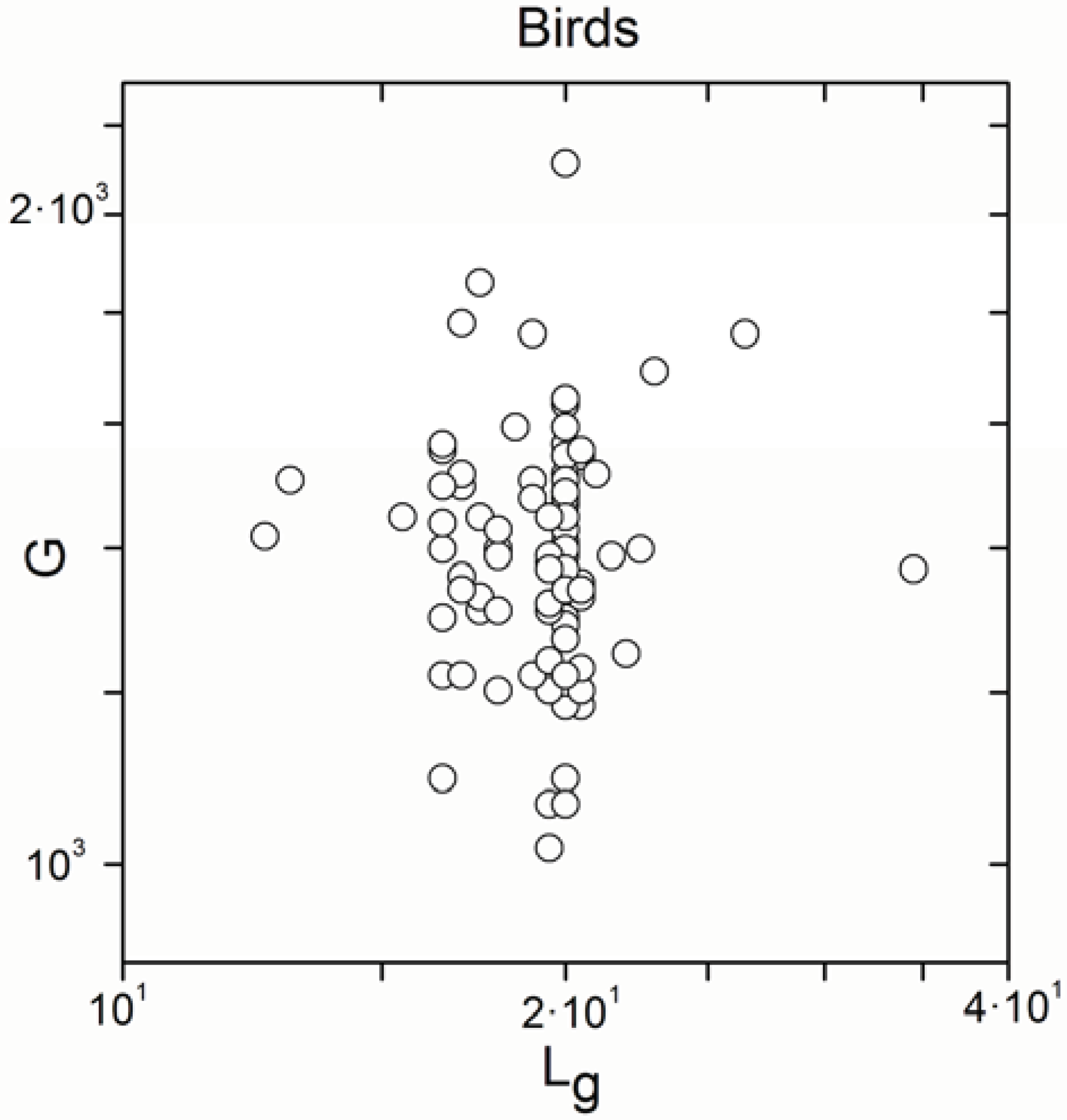
| Birds | 99 | 0.008 | 0.9 |
| Mammals | 371 | 0.297 | 5 × 10⁻⁹ |
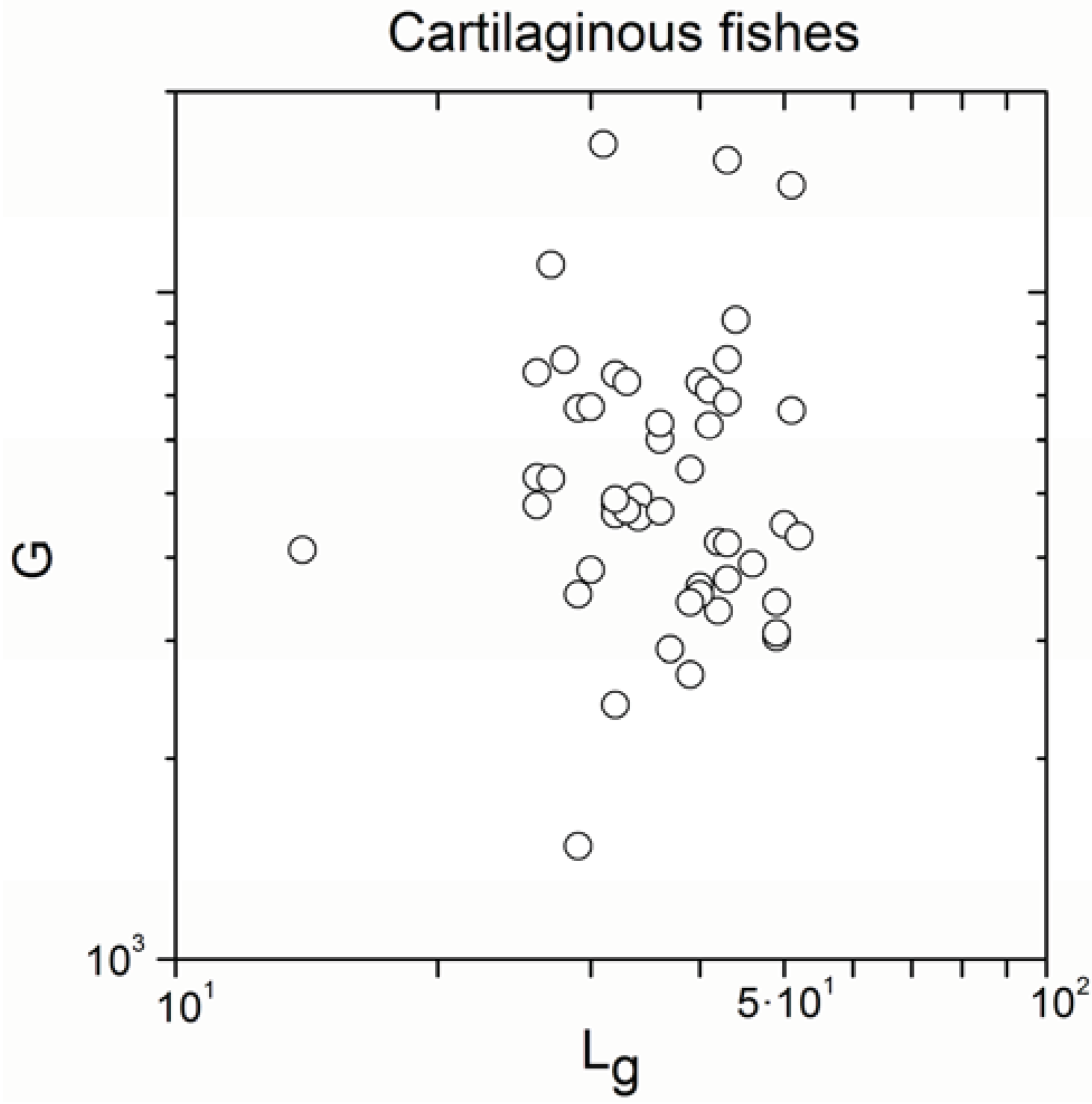
| Cartilaginous fishes | 52 | −0.129 | 0.4 |
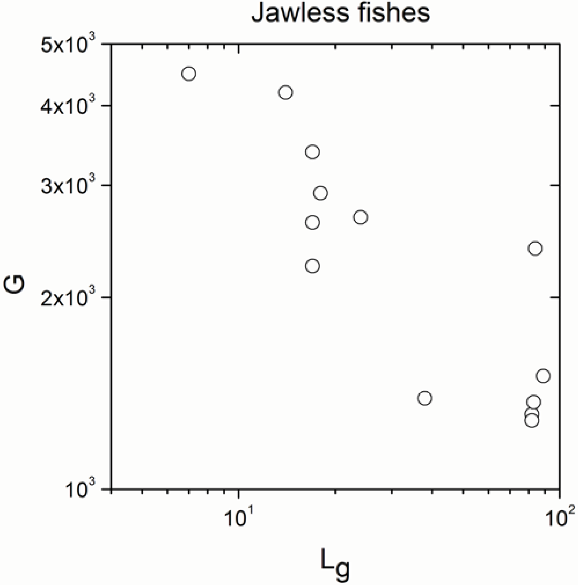
| Jawless fishes | 13 | −0.744 | 0.004 |
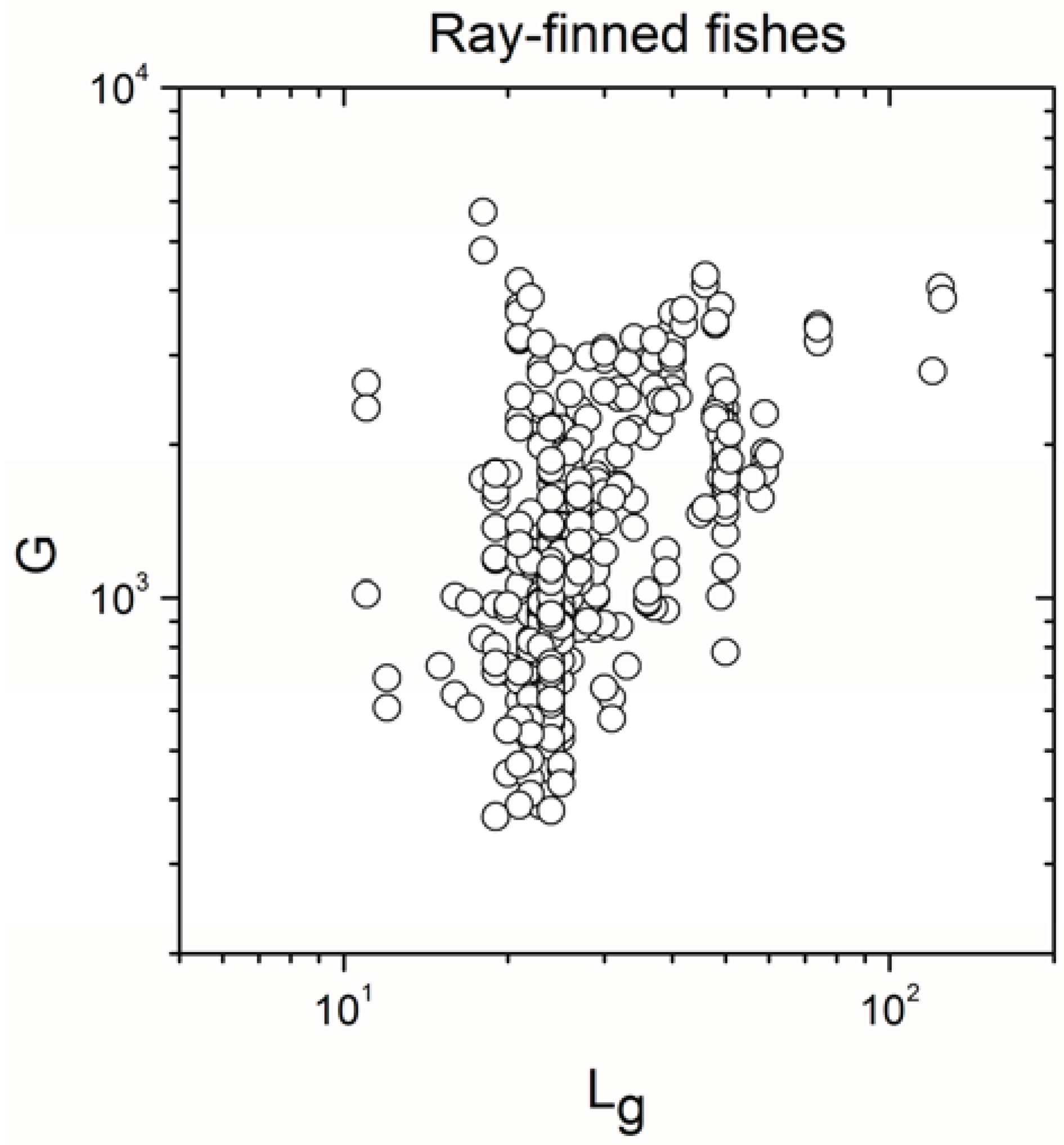
| Ray-finned fishes | 647 | 0.487 | <10−17 |
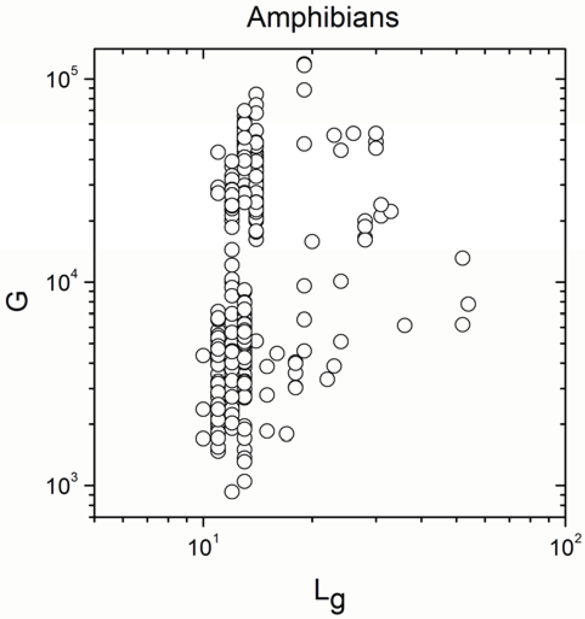
| Amphibians | 315 | 0.446 | 9 × 10⁻¹⁷ |
| Group | N | ρ | p |
|---|---|---|---|
| Fungi | 56 | 0.666 | 2 × 10⁻⁸ |
| Angiosperm plants | 4706 | 0.925 | <10−17 |
| Gymnosperm plants | 170 | 0.992 | <10−17 |
| Insects | 269 | 0.802 | <10−17 |
| Reptiles | 170 | 0.791 | <10−17 |
| Birds | 99 | 0.771 | <10−17 |
| Mammals | 371 | 0.278 | 5 × 10⁻⁸ |
| Cartilaginous fishes | 52 | 0.886 | <10−17 |
| Jawless fishes | 13 | 0.951 | <10−17 |
| Ray-finned fishes | 647 | 0.812930 | <10−17 |
| Amphibians | 315 | 0.983 | <10−17 |
3. Discussion
- G is chosen uniformly at random within the interval (Gm, GM).
- Lg (the number of chromosomes of the organism) is chosen uniformly at random within the interval (Lgm, LgM).
4. Methods
4.1. Data
4.2. A Test of Pure Linearity between G and Lg
- It does not assume that all the errors are only in the y-direction.
- It does not assume that either the x- or y-direction errors are normally distributed.
- It is robust in the sense that it is not affected by the presence of outliers.
Acknowledgments
References and Notes
- Vinogradov, A.E. Mirrored genome size distributions in monocot and dicot plants. Acta Biotheoretica 2001, 49, 43–51. [Google Scholar] [CrossRef] [PubMed]
- Trivers, R.; Burt, A.; Palestis, B.G. B chromosomes and genome size in flowering plants. Genome 2004, 47, 1–8. [Google Scholar] [CrossRef] [PubMed]
- Sankoff, D.; Ferretti, V. Karyotype distributions in a stochastic model of reciprocal translocation. Genome Res. 1996, 6, 1–9. [Google Scholar] [CrossRef] [PubMed]
- De, A.; Ferguson, M.; Sindi, S.; Durrett, R. The equilibrium distribution for a generalized Sankoff-Ferretti model accurately predicts chromosome size distribution in a wide variety of species. J. Appl. Probab. 2001, 38, 324–334. [Google Scholar] [CrossRef]
- Solé, R.V. Genome size, self-organization and DNA’s dark matter. Complexity 2010, 16, 20–23. [Google Scholar] [CrossRef]
- Ferrer-i-Cancho, R.; Forns, N. The self-organization of genomes. Complexity 2009, 15, 34–36. [Google Scholar] [CrossRef]
- DeGroot, M.H. Probability and Statistics, 2nd ed.; Addison-Wesley: Reading, MA, USA, 1989; p. 215. [Google Scholar]
- Gregory, T.R. Genome size evolution in animals. In The Evolution of the Genome; Gregory, T.R., Ed.; Elsevier: San Diego, CA, USA, 2005; pp. 4–71. [Google Scholar]
- Altmann, G. Prolegomena to Menzerath’s law. Glottometrika 1980, 2, 1–10. [Google Scholar]
- Boroda, M.G.; Altmann, G. Menzerath’s law in musical texts. Musikometrika 1991, 3, 1–13. [Google Scholar]
- Fuquan, K.; Kui, Z.; Yong, Z.; Tianguang, C.; Meinan, N.; Li, S.; Minghui, C.; Yizhong, Z. Analysis of length distribution of short DNA fragments induced by 7Li ions using the random-breakage model. Chin. Sci. Bull. 2005, 50, 841–844. [Google Scholar] [CrossRef]
- Becker, T.S.; Lenhard, B. The random versus fragile breakage models of chromosome evolution: A matter of resolution. Mol. Genet. Genomics 2007, 278, 487–491. [Google Scholar] [CrossRef] [PubMed]
- Schubert, I. Chromosome evolution. Curr. Opin. Plant Biol. 2007, 10, 109–115. [Google Scholar] [CrossRef] [PubMed]
- Li, X.; Zhu, C.; Lin, Z.; Wu, Y.; Zhang, D.; Bai, G.; Song, W.; Ma, J.; Muehlbauer, G.J.; Scalon, M.J.; et al. Chromosome size in diploid eukaryotic species centers on the average length with a conserved boundary. Mol. Biol. Evol. 2011. [Google Scholar] [CrossRef] [PubMed]
- Ritz, C.; Streibig, J.C. Nonlinear Regression with R; Springer: New York, NY, USA, 2008. [Google Scholar]
- Miller, J.C.; Miller, J.N. Statistics for Analytical Chemistry, 3rd ed.; Prentice Hall: London, UK, 1993; pp. 159–161. [Google Scholar]
- Pearl, J. Causality: Models, Reasoning, and Inference; Cambridge University Press: Cambridge, UK, 2000. [Google Scholar]
Appendix A


Appendix B
| Kingdom | Phylum/Division | Class | Order | Family | Genus |
|---|---|---|---|---|---|
| Fungi + 56 | 0,3,5 0,55 | 0,4,5 0,34 | 0,1,40 0,5 | ||
| Plants | Angiosperm − 4706 | 22,7,194 2374,965 | 66,8,1114 1608,186 | ||
| Gymnosperm + 170 | 0,4,14 0,122 | 0,2,52 0,13 | |||
| Animals | Arthropoda | Insects + 269 | 3,1,7 189,56 | 0,1,26 0,13 | |
| Chordata | Reptiles + 170 | 0,0,4 0,0 | 1,1,34 14,18 | ||
| Birds ? 99 | 0,0,17 0,0 | 0,0,33 0,0 | |||
| Mammals + 371 | 2,1,17 162,54 | 5,0,63 89,0 | |||
| Cartilaginous fishes ? 52 | 0,1,9 0,24 | 1,0,20 7,0 | |||
| Jawless fishes − 13 | 0,0,2 0,0 | 0,0,2 0,0 | 0,0,2 0,0 | ||
| Ray finned fishes + 647 | 4,0,30 262,0 | 3,0,115 214,0 | |||
| Amphibians + 315 | 1,0,3 185,0 | 3,1,26 42,72 |
- The sign of the significant correlations was totally reversed, in full agreement with definition (a) of Simpson’s paradox, only in fungi and gymnosperm plants.
- The sign of the significant correlation was totally maintained only in ray-finned fishes.
- The significant correlation was lost in jawless fishes, in agreement with definition (b) of the paradox.
- Significant correlations became a mixture of positive and negative correlations in angiosperm plants, insects, reptiles, mammals and amphibians.
- Non-significant correlations remained totally for birds.
- Significant correlations emerged only exceptionally in cartilaginous fishes (the number of significant correlations was very small with regard to the total number of subgroups), consistently with definition (b) of the paradox, but the sign of the correlation was not coherent.
© 2011 by the authors; licensee MDPI, Basel, Switzerland. This article is an open access article distributed under the terms and conditions of the Creative Commons Attribution license (http://creativecommons.org/licenses/by/3.0/).
Share and Cite
Hernández-Fernández, A.; Baixeries, J.; Forns, N.; Ferrer-i-Cancho, R. Size of the Whole versus Number of Parts in Genomes. Entropy 2011, 13, 1465-1480. https://doi.org/10.3390/e13081465
Hernández-Fernández A, Baixeries J, Forns N, Ferrer-i-Cancho R. Size of the Whole versus Number of Parts in Genomes. Entropy. 2011; 13(8):1465-1480. https://doi.org/10.3390/e13081465
Chicago/Turabian StyleHernández-Fernández, Antoni, Jaume Baixeries, Núria Forns, and Ramon Ferrer-i-Cancho. 2011. "Size of the Whole versus Number of Parts in Genomes" Entropy 13, no. 8: 1465-1480. https://doi.org/10.3390/e13081465