Spectral Entropy in a Boundary-Layer Flow

Professor Emeritus of Mechanical Engineering, University of Utah, 2067 Browning Avenue, Salt Lake City, UT 84108, USA
Entropy 2011, 13(9), 1555-1583; https://doi.org/10.3390/e13091555
Submission received: 15 July 2011
/
Revised: 20 August 2011
/
Accepted: 23 August 2011
/
Published: 26 August 2011
(This article belongs to the Special Issue Entropy Generation Minimization)
Abstract
:This article presents a comparison of the entropy production in a laminar and transitional boundary layer flow with the spectral entropy produced in a region of instability induced by an imposed periodic disturbance. The objective of the study is exploratory in nature by computing a boundary-layer environment with well-established computer techniques and comparing the predictions of the maximum rate of entropy production in the wall shear layer with the deterministic prediction of the spectral entropy growth within an inceptive instability in the inner region of the upstream boundary-layer flow. The deterministic values of the spectral entropy within the instability are brought into agreement with the computed rate of entropy production inversely along the shear flow with the assumption that the instability is of a span-wise vortex form and that the spectral entropy components are transported into the wall shear layer by vortex down sweep and are processed into thermodynamic entropy in the boundary-layer wall region.
Keywords:
boundary-layer computations; boundary layer entropy production; induced flow instabilities; spectral entropy; vortex-induced down sweepPACS Codes:
05.45.Pq (Numerical simulation of chaotic systems); 05.70.Ce (Entropy); 47.15.Cb (Laminar boundary layers); 47.15.Fe (Stability of boundary layers); 47.27.nb (Boundary layer turbulence); 47.32.ck (Vortex streets)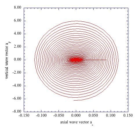
1. Introduction
The engineering computation of the flow of an ideal gas along a wall shear layer is a highly developed field in computational fluid dynamics. Cebeci and Bradshaw [1,2], Cebeci [3], Cebeci and Cousteix [4] have published a series of books that provide detailed descriptions of computed flow configurations. A number of effective computer programs for the computation of boundary-layer flows are based upon the Keller box method, fully described in [1]. Our objective here is to use the Keller box method computing environment as developed and documented by in [1,2,3,4] to compute the entropy production along a wall shear layer of the Falkner-Skan type. The velocity profiles in three-dimensions are computed at an upstream laminar region and then used in the computation of the wall production of the local entropy production. This computing environment is used to calculate the local entropy production in the downstream direction to obtain entropy production rates in both the laminar and transitional regions of the flow.
A model of the flow equations describing the fluctuating velocity components as developed by Townsend [5] is used to predict the presence of a region of induced instability in the inner region of the laminar shear layer. Isaacson [6,7] has presented a modification of the Townsend flow equations that includes the nonlinear coupling terms. The spectral entropy predicted from the solution of these time-dependent fluctuation equations may be connected to the actual entropy increase observed in the wall regions of the boundary-layer flow.
Finally, the physics of the connection of the flow structures producing the spectral entropy values in the flow instability region with the entropy production in the boundary-layer wall region is addressed.
From the computational results of the modified Townsend equations in the laminar instability region, phase diagrams of the axial and vertical velocity fluctuations with the span wise velocity fluctuations indicate that the flow structures may be of the span wise roll vortex type. We use this observation to employ a computational procedure developed by Chow [8] to compute the induced down sweep of the appropriate fluctuating flow element of a given spectral entropy into the corresponding region of computed wall production of entropy. The axial distance for the computation of the induced down sweep is determined from the distance to the corresponding value of entropy production in the wall shear layer region.
2. Boundary-Layer Flow Environment
The basic objective of this study is to use the boundary layer flow environments computed with well-established computational tools to establish a basis of a set of entropy production values calculated along a transitional region of a boundary layer flow. Cebeci and Bradshaw [1,2], Cebeci and Cousteix [3], and Cebeci [4] have developed a set of computer source codes for the computation of various wall shear layer environments. These source codes have been used to create computer programs required to compute the desired boundary layer flows, including the necessary gradients in the mean velocities in a three-dimensional configuration. All of the computations in this article were accomplished in the C programming language using a Macintosh OSX computing environment.
2.1. Computational Model for the Boundary-Layer Flow
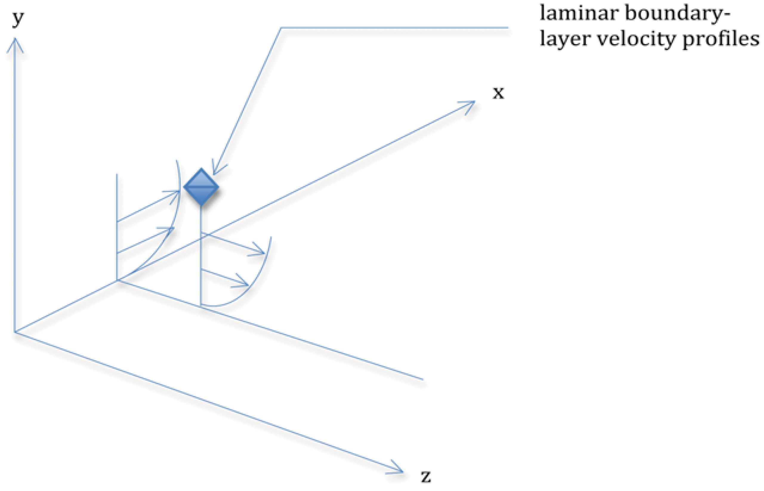
The flow configuration we wish to model is the three-dimensional wall shear layer downstream of an initial starting plane, as indicated in Figure 1. The flow is from left to right and is assumed to be an ideal gas moving at supersonic velocity over a flat plate with laminar, transitional, and turbulent flow.
The computational procedure developed by Cebeci and Bradshaw [1] is used as the basis for our computations of the boundary layer flow. The flow is of the Falkner-Skan type with an adverse pressure gradient, enhancing the transition from laminar to turbulent flow. The modification, which we introduce, is to impose an initial free stream velocity of unity, making the boundary layer edge velocity dimensionless. The main computer program in the computational procedure developed by Cebeci and Bradshaw [1] establishes “nx” as the station number for the axial direction and the symbol “j” for the vertical grid number for the calculation of the vertical profiles at a given axial station. Following the nomenclature used in the computer program development, we will use “nx” throughout this article to identify the axial station calculations and the vertical grid number “j” to specify the values of the appropriate vertical parameters. We also will include the corresponding axial distance with the nx value and the corresponding η value with the vertical station number j.
Figure 1.
The three-dimensional flow model and the coordinate system for the boundary layer flow environment. Note the location for the laminar flow velocity profile computations.
Figure 1.
The three-dimensional flow model and the coordinate system for the boundary layer flow environment. Note the location for the laminar flow velocity profile computations.

In an analysis of the conditions for similarity in boundary layer flows, Hansen [9] indicates that both the Blasius profile of the velocity gradient in the x-y plane and the Blasius profile in the z-y plane along the original starting planes are similar. Hence, we apply the computer methods of Cebeci and Bradshaw [1] to the computation of the laminar velocity profile in the x-y plane at the axial station, nx = 4 (x = 0.08), along the x-axis, and the same computer methods to the computation of the laminar velocity profile in the z-y plane at the span wise station, nz = 4 (z = 0.08), along the z-axis.
It is assumed that the velocity profiles in the z-y plane remain laminar as the computations move in the axial direction. Therefore, only the velocity gradients computed in the z-y location at the span wise station nz = 4 (z = 0.08) are used in the computation of the entropy production in the wall shear layer in the axial direction.
However, it is noted that the flow in the axial direction is assumed to be laminar at the axial station of nx = 4 (x = 0.08), undergoes the initiation of transition at nx = 8 (x = 0.16), and then develops the transitional process from this station downstream as x increases. The production of entropy in the wall shear region is then computed at the axial stations of nx = 4 (x = 0.08), nx = 10 (x = 0.16), nx = 18 (x= 0.36), and nx = 36 (x = 0.72). These entropy production values then serve as a basis of comparison for the spectral entropy values which are computed at transformed vertical stations of j = 2 (η = 0.200), j = 10 (η = 1.804), j = 14 (η = 2.608), j = 18 (η = 3.414), and j = 22 (η = 4.221) at the axial station of nx = 4 (x = 0.08) and the span wise station of nz = 4 (z = 0.08).
Since the mathematical and computational procedures for the computation of the boundary layer flow are fully developed and described in [1,2,3,4], only an outline of the boundary-layer computational procedure is presented here. Where we have used expressions for mean velocity gradients that do not appear in these references, we provide more detail. The momentum equations for the boundary-layer flow may be written as:
where the meaning of each of the symbols is given in the Nomenclature.
The boundary conditions are:
For application to thin shear layers that include laminar, transitional, and turbulent regions, the Reynolds shear stress is modeled with the “eddy viscosity” formula, which defines a quantity , having the dimensions of (viscosity) / (density), by:
Following Cebeci and Bradshaw, the Falkner-Skan transformation is defined by:
The velocity at the edge of the boundary layer, , is assumed to vary with distance x. A dimensionless stream function, , is introduced and is given by:
These definitions yield the results for velocities u and v as:
In these expressions, the prime indicates differentiation with respect to .
Replacing the pressure gradient term by and defining the parameter m as:
Cebeci and Bradshaw write the transformed momentum equation for the thin plane shear layer as:
where:
The boundary conditions for this expression are, with no surface mass transfer:
To implement the numerical solution of this third-order differential equation, the Keller-Cebeci box method replaces it with three first-order differential equations in the following fashion:
The boundary conditions for these three equations are:
f(x,0) = 0 u(x,0) = 0 u(x,η∞) = 1
Note that in Equations (14) and (15), v is not the y-component velocity.
The boundary-layer computer program developed by Cebeci and Bradshaw [1] consists of a MAIN driver routine and eight subroutines that implement the various parts of the program. The subroutines are as follow: INPUT provides the input values of the kinematic viscosity ν and the transformed vertical dimension η at nx = 1 (x = 0.02) and ue, and m as functions of the axial direction x; GRID generates the computational grid across the boundary layer; IVPL generates the initial velocity profile for the laminar portion of the flow; the GROWTH subroutine provides for the growth of the boundary layer; EDDY contains the expressions for the inner and outer eddy viscosity formulations used in the transitional and turbulent portions of the flow; CMOM computes the coefficients of the differenced form of the transformed momentum equation; SOLV3 calculates the recursion formulas that occur in the block elimination of the Keller-Cebeci box method; and OUTPUT provides the output of the computations for the boundary-layer parameters and profiles. The computational data output is stored on external data files for access by the remaining computational procedures in this project.
The implementation of the calculations for the local production of entropy within the boundary-layer flow requires the evaluation of velocity gradients in a three-dimensional format. We have again followed the procedure of Cebeci and Bradshaw [1] in implementing a computational procedure for the development of the boundary layer along the z-y plane as indicated in Figure 1. Here, however, we uncouple the x-y plane boundary-layer development from the z-y plane and apply the same computer procedure as outlined above to the flow along the z-y plane at the initial laminar region of nx = 4 (x = 0.08), where nx is the axial station number for the development of the initial laminar flow in the axial direction and nz = 4 as the corresponding location in the z-direction. This procedure thus yields the necessary velocity gradients in the z-y plane for both the computations of the local production of entropy within the shear layer and the computation of the unsteady velocity fluctuations in the unstable region of the boundary-layer flow.
In addition to the normal velocity profiles across the boundary layer, gradients in the various flow velocities are also needed. The set of velocity gradients required are the following:
With the assumption that the velocity profiles in the z-y plane are independent of the profiles in the x-y plane, we may write:
From the continuity equations in both the x-y plane and in the z-y plane, we may write:
Utilizing the transformed variables from [1], the appropriate velocity gradients are obtained from the computational output with the following equations:
In these expressions, the prime indicates differentiation with respect to η. Corresponding expressions are used to determine similar velocity gradients in the z-y plane.
We have chosen the flow environment presented by Cebeci and Bradshaw [1] in their Example 8A.1, which is a two-dimensional incompressible boundary layer flow, initially laminar, but which we allow to undergo transition into a turbulent flow. This example was chosen as a base computational environment with which to compare our computations. A particular set of flow conditions that correspond to this base environment is an atmospheric flight Mach number of 1.44 at an altitude of 30 km which yields a stagnation temperature T0 = 307.0 K and a stagnation pressure P0 = 10132.5 N/m2. These values yield a kinematic viscosity of 1.64 × 10⁻⁴ m2/s. To simplify the approach to the computational process, we consider this value of the kinematic viscosity as applicable to boundary layers of interest and thus use this value throughout the boundary layer calculations. The density is calculated from the ideal gas equation of state and the dynamic viscosity for air is calculated from the expression given by Zucrow and Hoffman [10]. These values then yield the kinematic viscosity value close to that used in the example program of [1]. We have chosen this approach to allow a straightforward application of the methods of [1] to the numerical solution of the equations describing the basic flow environment.
The basic flow environment that we compute corresponds to a flow with the external velocity given by:
In this expression, ue is the dimensionless edge velocity and x is the dimensionless axial distance. The corresponding pressure gradient parameter, m, is given by
We start the computations at nx = 4 (x = 0.08), thus initially computing the boundary layer as laminar. We take the total number of axial stations, nxt = 50 (x = 1.00), with transition occurring at the axial station ntr = 8 (x = 0.16). The length of the plate is taken as 1.0 m.
For the flow in the z direction, we take the external velocity we = 0.01, with a pressure gradient of zero in the z direction. The computations are made at a span wise station of nz = 4 (z = 0.08), at the axial station of nx = 4 (x = 0.08), with the span wise results held constant as the computations proceed in the axial direction. This procedure allows us to estimate the required velocity gradients at the initially laminar region in a three-dimensional configuration, as indicated in Figure 1.
2.2. Entropy Production within the Boundary-Layer Flow
One of the primary objectives of this study is to provide a basis of computations of the entropy production within the specified boundary-layer flow. Expressions for the energy dissipation by the various velocity gradients within a laminar shear layer have been developed by a number of authors, including [11,12,13,14,15]. Several of these authors, Truitt [13] and Bejan [14], have extended the expressions for energy dissipation to the volume rate of production of local entropy.
For a three-dimensional system without temperature gradients, we may write the approximate volumetric entropy production rate equation for the viscous region [13] as:
Assuming the independence of the gradients in the x-y and the z-y planes (Equation (18)), the expression for the entropy generation rate per unit mass in the laminar region may then be written in the form:
The ideal gas law may be written in the form:
Substitution of the temperature from this equation into Equation (27) yields the expression for the dimensionless rate of entropy production (1/s) due to viscous shear stresses as:
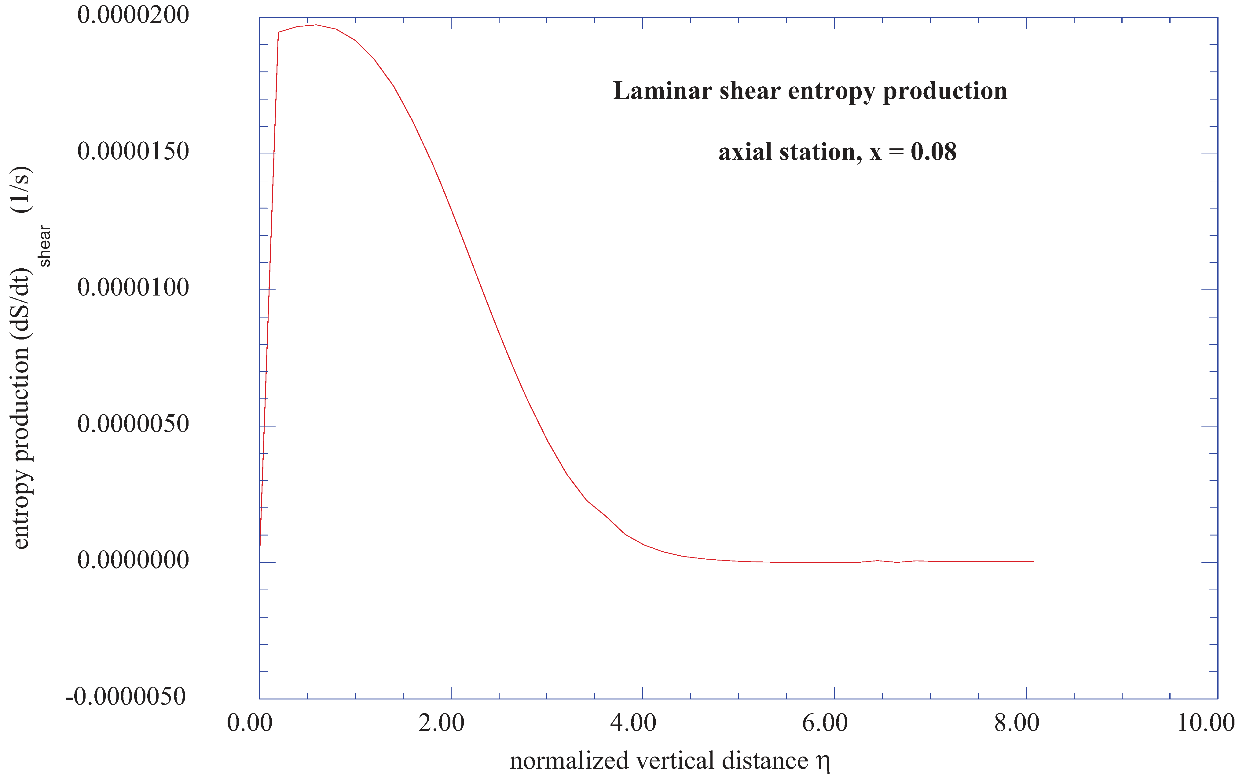
Using the values for the various velocity gradients obtained from the computer solutions, the results of the computation of the dimensionless rate of entropy production in the laminar region of the boundary-layer flow at the axial station, nix = 4 (x = 0.08) and the span wise station of nz = 4 (z = 0.08) is shown in Figure 2.
Figure 2.
The dimensionless rate of entropy production in the laminar boundary layer at the axial station nx = 4 (x = 0.08) and the span wise station nz = 4 (z = 0.08).
Figure 2.
The dimensionless rate of entropy production in the laminar boundary layer at the axial station nx = 4 (x = 0.08) and the span wise station nz = 4 (z = 0.08).
The production of entropy in the viscous flow region is assumed to occur on the molecular scale of the flow of the working gas. The flow is assumed to possess an axial mean velocity in the free-stream. The no-slip condition for the gas at the wall surface assumes that this axial momentum is brought to zero at the surface. We may assume that the entropy of the molecular state with zero axial velocity is a maximum in the thermodynamic sense, and that the entropy of flow elements that have components of axial velocity are at a lower entropy state. Thus, the production of molecular-level entropy in the wall region is brought about by the irreversible dissolution of the directed kinetic energy of the flow velocity by the viscous shear stresses resulting from the no-slip condition imposed at the surface. Since the flow is assumed to be laminar, molecular processes bring about the dissolution of directed kinetic energy across laminar layers, not by the transport of macroscopic flow elements [16,17,18,19,20].
For flows that exhibit intermittency and turbulent behavior, the concepts of intermittency and eddy viscosity are introduced [22,23,24]. The concept of eddy viscosity is actually defined by Equation (4), with measured values of the turbulent shear stress, , divided by the measured mean velocity gradient, . In the expression for the turbulent shear stress, u’ and v’ are fluctuations of macroscopic elements of the axial and vertical velocity components. These fluctuations are reflective of macroscopic heat transfer processes for the constant-temperature hot-wire anemometry system used to obtain the measurements. The values of these fluctuations are much higher than the diffusive processes that take place in the laminar case. The flow elements that produce these fluctuations thus contain considerable levels of directed kinetic energy associated with the axial and vertical velocity directions. Again, for an adiabatic wall, (equilibrium of surface temperature with the adjacent gas layer), this layer will have maximum entropy. Those fluid elements away from the wall will have macroscopic deviations from a uniform distribution, and thus will have lower values of entropy [25,26,27]. The production of entropy in the intermittent and eddy viscosity cases will involve the irreversible dissolution of the directed kinetic energies of the macroscopic elements brought into the wall region of the flow. In this sense, the turbulent regions of the flow are more ordered than the laminar regions. The essential point here is that the turbulent regions of the flow contain macroscopic flow elements with considerable levels of directed kinetic energy, serving as the source for the production of entropy in the wall region.
The entropy generation rate in the transitional and turbulent regions of the boundary layer flow is assumed to be dominated by the eddy viscosity term and may be written as:
Combining Equations (4), (10), and (21), the dimensionless entropy generation rate (1/s) in the transitional and turbulent regions of the flow becomes:
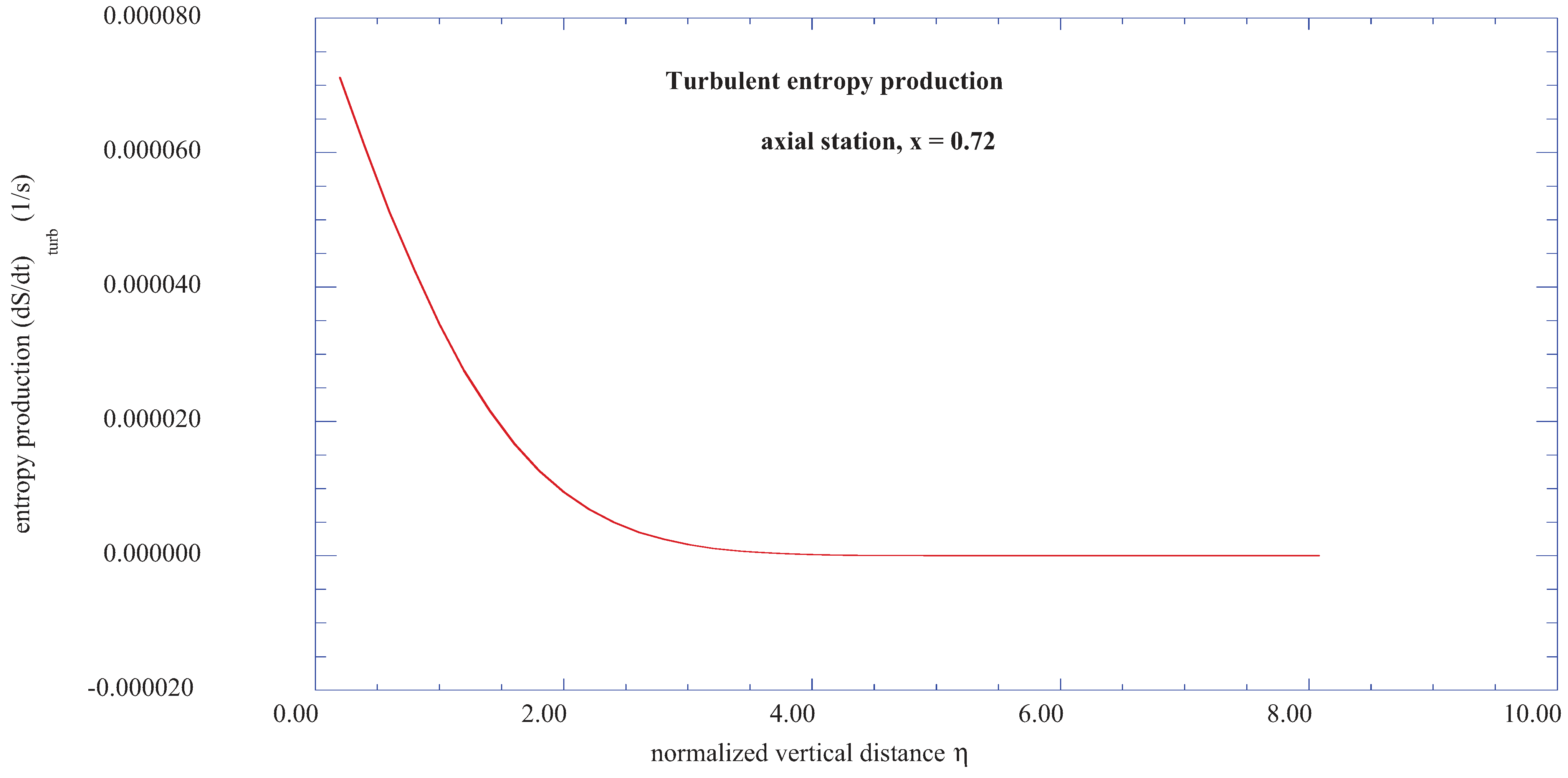
The dimensionless production rates for the entropy in the transitional and turbulent regions of the flow are presented in Figure 3, Figure 4 and Figure 5. The axial station values for these results are nx = 10 (x = 0.20), nx = 16 (x = 0.32), and nx = 36 (x = 0.72). Note that the entropy production rate in the wall region at the transitional station of nx = 10 (x = 0.20) is nearly 20 times greater than the laminar rate at the axial station of nx = 4 (x = 0.08).
Figure 3.
The dimensionless rate of entropy production in the transitional boundary layer at the axial station, nx = 10 (x = 0.20) and the span wise station nz = 4 (z = 0.08).
Figure 3.
The dimensionless rate of entropy production in the transitional boundary layer at the axial station, nx = 10 (x = 0.20) and the span wise station nz = 4 (z = 0.08).
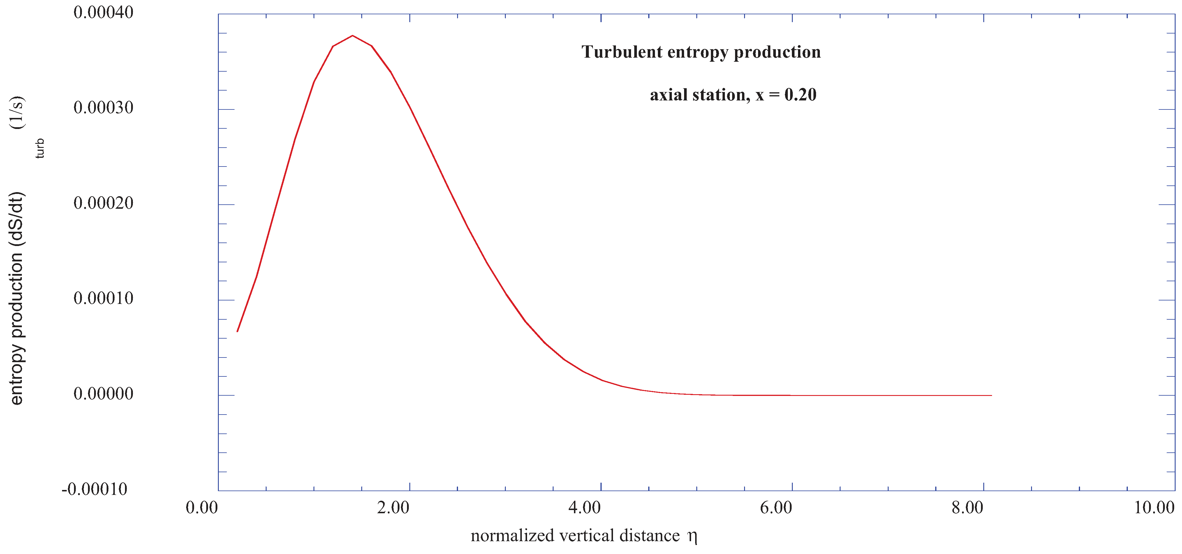
Figure 4.
The dimensionless rate of entropy production in the transitional boundary layer at the axial station, nx = 16 (x = 0.32) and the span wise station nz = 4 (z = 0.08).
Figure 4.
The dimensionless rate of entropy production in the transitional boundary layer at the axial station, nx = 16 (x = 0.32) and the span wise station nz = 4 (z = 0.08).
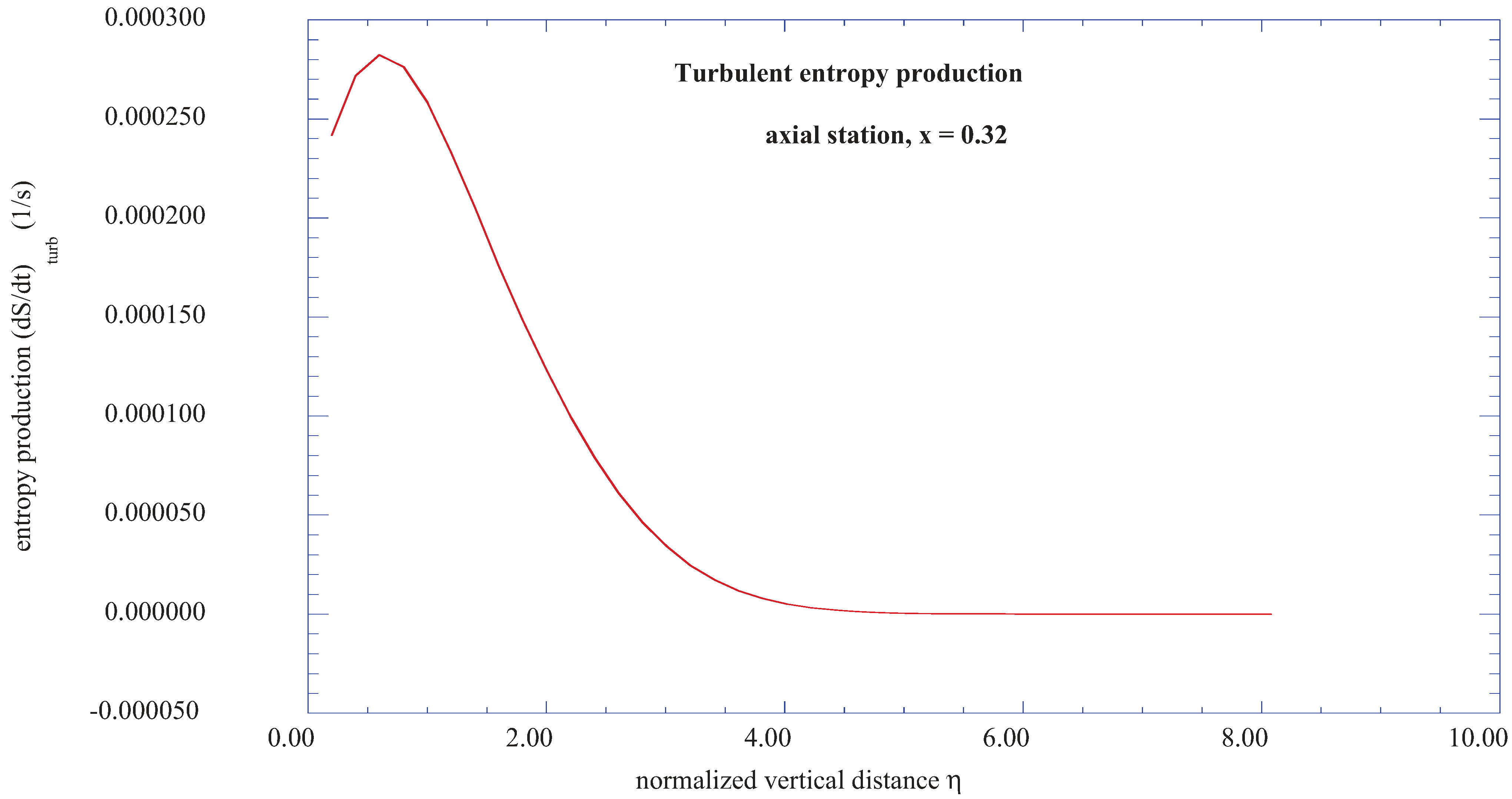
Figure 5.
The dimensionless rate of entropy production in the transitional boundary layer at the axial station, nx = 36 (x = 0.72) and the span wise station, nz = 4 (z = 0.08).
Figure 5.
The dimensionless rate of entropy production in the transitional boundary layer at the axial station, nx = 36 (x = 0.72) and the span wise station, nz = 4 (z = 0.08).
3. Mathematical Model of the Flow Instability
3.1. Transformation of the Townsend Equations
Crepeau [28] studied the behavior of the spectral entropy in the axial direction of a transitional boundary layer for a specified vertical location (η = 5.0), with the Reynolds number based on the axial distance x as the control parameter. A modified form of the Townsend equations was used to calculate the spectral entropy behavior in the boundary-layer flow. The results of this study imply the development of a fluid instability arising near the wall and propagating upwards. The important results obtained by Crepeau [28] warrant further investigation to evaluate the characteristics of the implied upward “burst” of instability through the boundary layer.
Considerable effort has recently been devoted to the study of the transition of laminar boundary layers brought about by the existence of free-stream disturbances. A thorough review of both mathematical and experimental results has been presented in the collection of articles edited by Gad-el-Hak and Tsai [29]. Recent work has been presented in [30,31,32,33,34]. These references present an extensive review of the recent work in this field and hence a review of this work will not be repeated here. However, several aspects of the so-called by-pass transition process are essential to our mathematical model and hence will be discussed here. One of the essential aspects of these studies is the evidence that strong free-stream turbulence produces elongated stream wise structures with narrow span wise scales. These disturbances apparently give rise to a periodic modulation of the stream wise velocity. We will use the results of [29,30,31,32,33,34] to further investigate the possibilities of the existence of vertical bursts occurring near the wall in a boundary-layer flow, as implied in the results of [28].
The Navier-Stokes equations describing this flow are transformed through a Fourier analysis into a Lorenz-type format, specifically keeping the nonlinear coupling terms. The coefficient of the nonlinear terms is simplified into a form obtained from the perturbation theory of non-relativistic quantum mechanics as described by Landau and Lifshitz [35]. Using the Fourier expansion procedure as presented by Townsend [5], the equations of motion for the boundary-layer flow may be separated into steady plus fluctuating values of the velocity components. The velocity fluctuations around the mean values of the velocity components will thus be of primary interest. The equations for the velocity fluctuations may be written as follows [5]:
In these equations, ν is the kinematic viscosity. The pressure term may be transformed as:
In these expressions, the mean velocity components are denoted by Ui, with i = 1,2,3 representing the x, y, and z components, while xj, with j = 1,2,3, denote the x, y, and z distances. The three mean velocity components and the nine gradients in the mean velocities are obtained from the solutions for the boundary-layer flow as outlined in previous sections.
As Townsend [5] points out, the pressure is determined by the velocity and temperature fields and is not a local quantity but depends on the entire field of velocity and temperature. The elimination of the pressure fluctuation term introduces nonlinear coupling between the velocity coefficients. In our work here, we will introduce an internal feedback mechanism that will model the nonlinear interaction process but will allow the resulting equations to be integrated in time. The velocity fluctuations may be expanded in terms of a sum of Fourier components as:
The variation with time of each Fourier component of the fluctuation field is then given by the equation for each of the velocity wave vector amplitudes:
The equations for the rate of change of the wave numbers are:
The equations for the fluctuating velocity components may be transformed by Fourier expansion into a form similar to Lorenz-type equations, as shown by Hellberg and Orszag [36] and Isaacson [6,7]. The equations resulting from the transformation process have been presented in other publications and references to them may be found in [6].
In the mathematical model used in this study, the coefficients in the set of differential equations for the variation of the wave numbers are replaced by periodic functions of the form cos(ω0t), where ω0 is an amplification factor for the frequency of the periodic disturbances. This set of equations forms a set of external control parameters, as discussed by Klimontovich [37]. A second set of internal control parameters is provided by the values of the mean velocity gradients determined in the solution of the boundary-layer flow as discussed in previous sections.
The computational solution of the nonlinear Townsend equations for the fluctuating components of the velocity wave vectors in our study is aided by the introduction of these two sets of feedback parameters. The first set of parameters is obtained by the ad hoc replacement of the gradients of the mean velocities that appear in Equation (36) by a periodic cosine function [37] as follows:
In these expressions, ω0 is an externally applied frequency factor, held constant at ω0 = 4.0 throughout the computations. The initial values for the wave numbers are:
kx (t = 0.0) = 0.80; ky (t = 0.0) = 0.1; kz (t = 0.0) = 0.1
With this approximation, we uncouple the continuity equations for the wave numbers from the solutions of the deterministic equations for the velocity fluctuation wave vectors. The solution of these equations for the time dependent wave numbers provides results that are stored in files available for input into the computational solutions of the deterministic equations for the fluctuating velocity coefficients. These results for the wave numbers represent the influence of the externally applied free-stream disturbances across all of the boundary layer vertical stations for which solutions of the deterministic equations will be sought.
A preliminary evaluation of the results of the computations of the deterministic equations for an amplitude of unity for the cosine functions and a frequency factor of ω0 = 4.0 yielded consistent results for the computations. However, for deterministic equations of the Lorenz-type, the results are very sensitive to the values of the external control parameters. We are therefore exploring the behavior of the computational results for the deterministic equations for various values of input amplitude of the cosine functions and for various values of the frequency factor. These results will be reported in a future paper.
The next approximation is to the set of first-order nonlinear differential equations describing the equations of motion of the fluctuating velocity components. We substitute the term as the coefficient of the nonlinear terms in the equations for the time rate of change of the coefficients. In this expression [38,39]:
where is an ad hoc adjustable weight of the perturbation and is the magnitude of the time-dependent wave vector given by:
The value for has been arbitrarily set to 0.10, which allows the computations to remain stable throughout the time step range for each of the vertical stations examined. Variations in the value of K1 will be examined in the on-going numerical study of the effects of the external control parameters on the solutions of the deterministic equations describing the flow instabilities.
The three deterministic equations for the velocity coefficients may then be written as:
Note that the perturbation factor is applied to the nonlinear terms in the equations for and , and not to one of the directly accessible dependent variables. This is a significant change from the practice in the study of synchronization and chaos [38,39]. The form of the perturbation factor and the application of the factor to the nonlinear terms are motivated by the perturbation analysis of the wave functions in non-relativistic quantum mechanics. This has been demonstrated by a specific example reported in [35]. The application of the perturbation factor in this fashion implies that the nonlinear terms in the first-order equations for the velocity fluctuations represent transition probabilities from an initial state to a secondary state.
The second set of feedback parameters [37] are internal to the boundary-layer flow and consists of the set of values obtained for the various mean velocity gradients at each vertical station, j (η), in the laminar boundary layer at the axial station nx = 4 (x = 0.08) and the span wise station nz = 4 (z = 0.08). The equations for the mean velocity gradients in the x-y and y-z planes of the boundary-layer flow are obtained from the solution of the boundary layer environment as described in previous sections. The computational results, stored in external files, provide the gradients of the various mean velocities at the specified vertical locations within the laminar boundary layer at the axial station nx = 4 (x = 0.08), with the computations at each vertical location proceeding from the wall surface to the outer boundary of the shear layer.
The theoretical modeling of the internal flow instabilities within the boundary-layer flow consists of six simultaneous first-order differential equations, to be solved at each vertical station within the wall shear layer. The mean velocity gradients are obtained at each vertical station from the overall solution of the boundary layer equations, together with the thermodynamic and viscous properties of the fluid involved. The solution of the set of equation describing the flow instabilities yields the velocity-fluctuation wave-vectors in three-dimensions for each of the vertical stations within the wall shear layer at the axial station of nx = 4 (x = 0.08). The initial values of the fluctuating velocity wave-vectors are:
The equations are integrated using a fourth-order Runge-Kutta technique with computer source codes as presented by Press et al. [40]. First, the three first-order differential equations for the wave numbers are integrated in time with the resulting series stored to files on the hard drive. A time step of 0.0001 s is used with a total of 12,288 time steps included in the integration process. The resulting time-series are stored in external data files. These data files thus become available for the spectral analysis as described in the next section.
Figure 6 indicates that a flow instability occurs very near the wall at the transformed vertical position of j = 2 (η = 0.200). With a time step for the integration of these equations equal to 0.0001, a very rapid development of the instabilities is indicated. Figure 7 plots the phase plane behavior of the vertical velocity wave vector, ay, versus the axial velocity wave vector, ax, for the transformed vertical location of j = 2 (η = 0.200). These results indicate that the effects of the external periodic disturbance are transmitted through the entire boundary layer structure. As indicated in both Figure 6 and Figure 7, the magnitudes of the ax and ay wave vectors are significant, thus representing a largely vertical burst of fluctuating fluid elements.
Figure 6.
The axial velocity wave vector, ax, as a function of time step at the transformed vertical station of j = 2 (η = 0.200).
Figure 6.
The axial velocity wave vector, ax, as a function of time step at the transformed vertical station of j = 2 (η = 0.200).
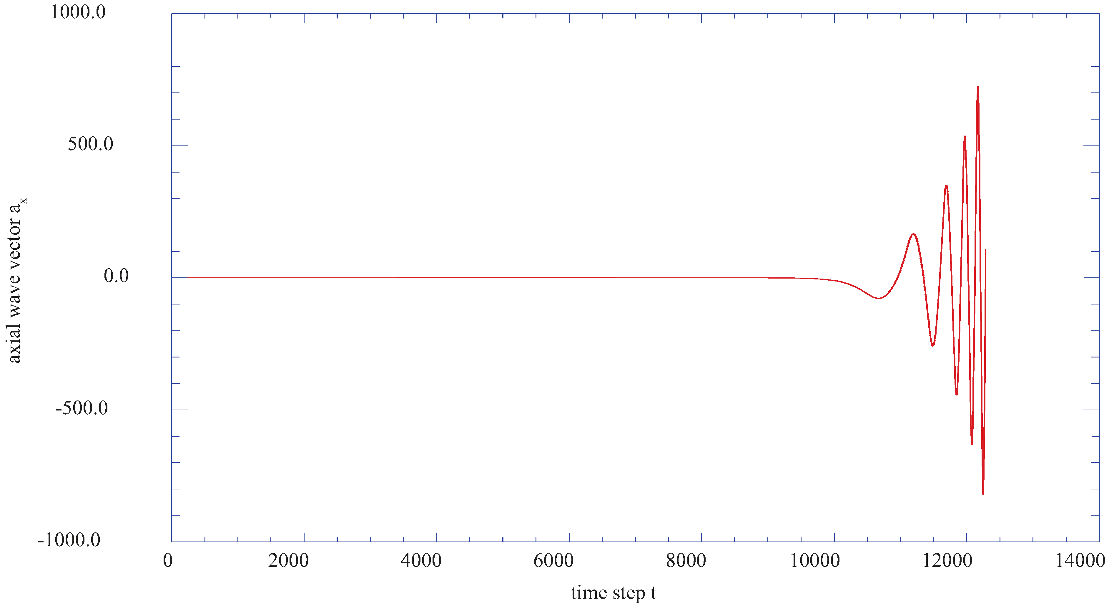
Figure 7.
The vertical component of the fluctuating wave vector, ay, versus the axial component, ax, for the vertical location of j = 2 (η = 0.200).
Figure 7.
The vertical component of the fluctuating wave vector, ay, versus the axial component, ax, for the vertical location of j = 2 (η = 0.200).

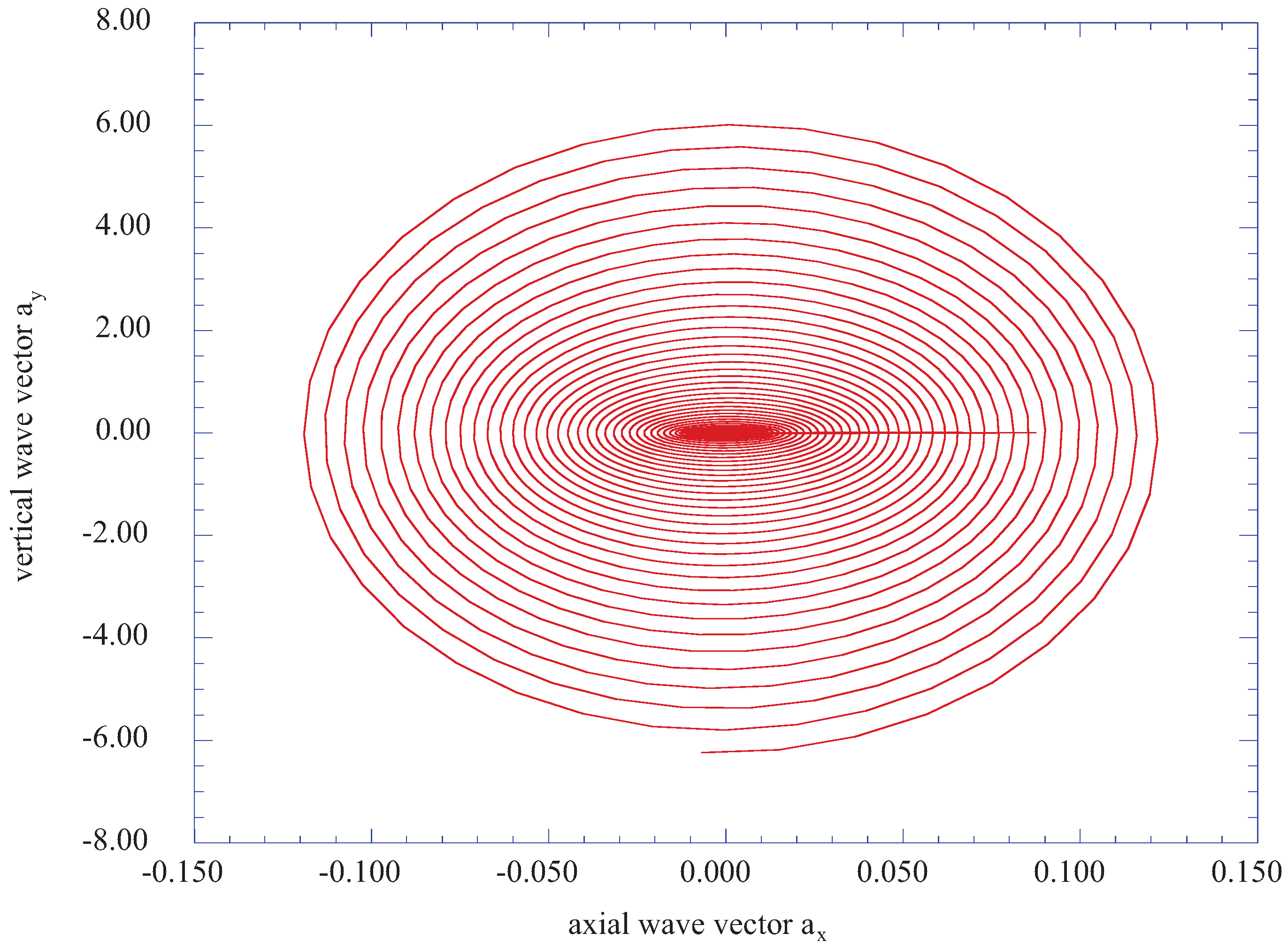
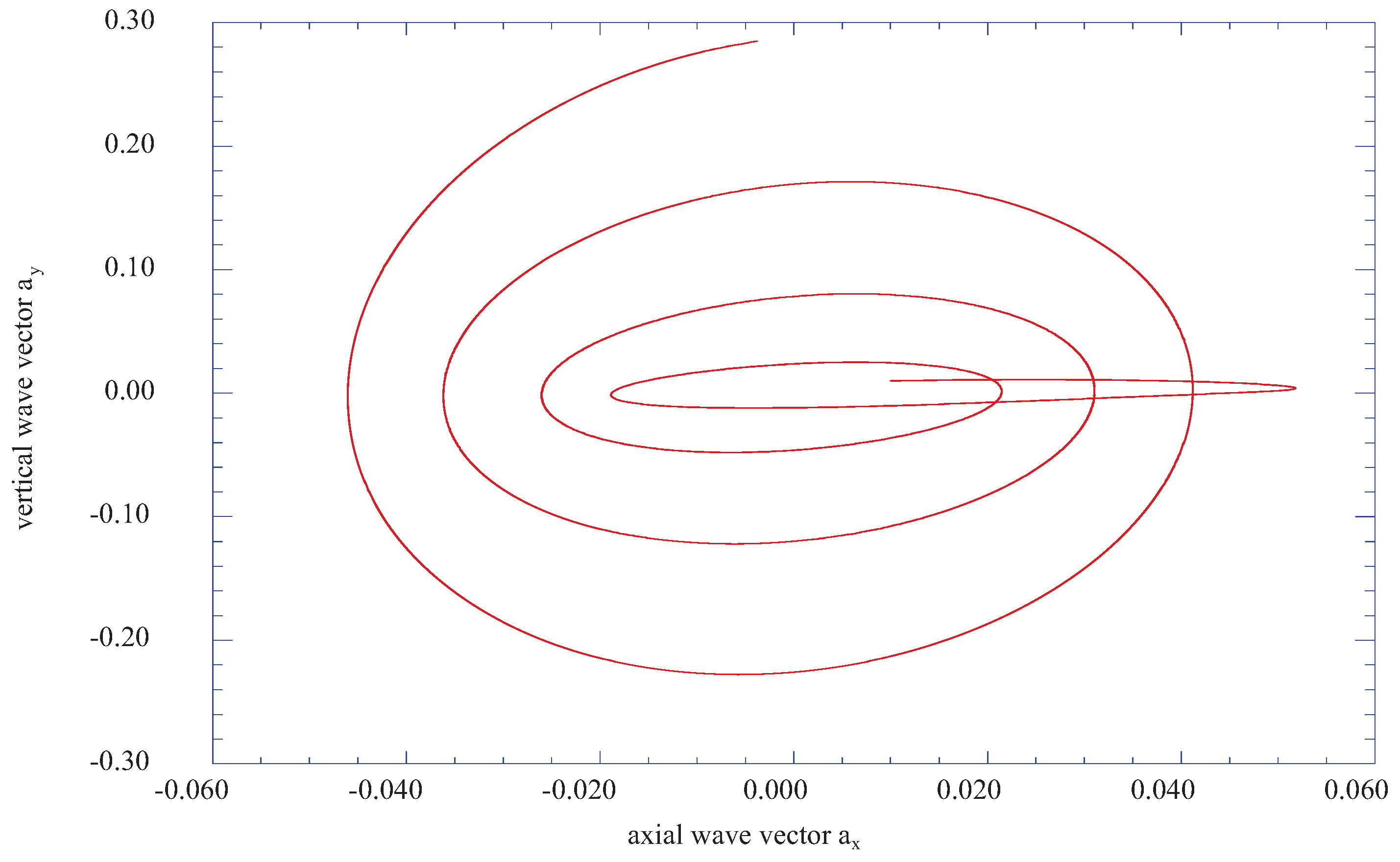
Figure 8 presents the phase plane plot for the vertical wave vector component, ay, versus the axial wave vector component, ax, for the vertical location of j = 10 (η = 1.804). These results indicate an oscillatory behavior in the vertical direction still much larger than the extent of the axial fluctuation. Again, these are results obtained within the laminar velocity profile at nx = 4 (x = 0.08).
Figure 8.
The vertical component of the fluctuating velocity wave vector, ay, as a function of the axial fluctuating wave vector, ax, at the vertical location of j = 10 (η = 1.804).
Figure 8.
The vertical component of the fluctuating velocity wave vector, ay, as a function of the axial fluctuating wave vector, ax, at the vertical location of j = 10 (η = 1.804).
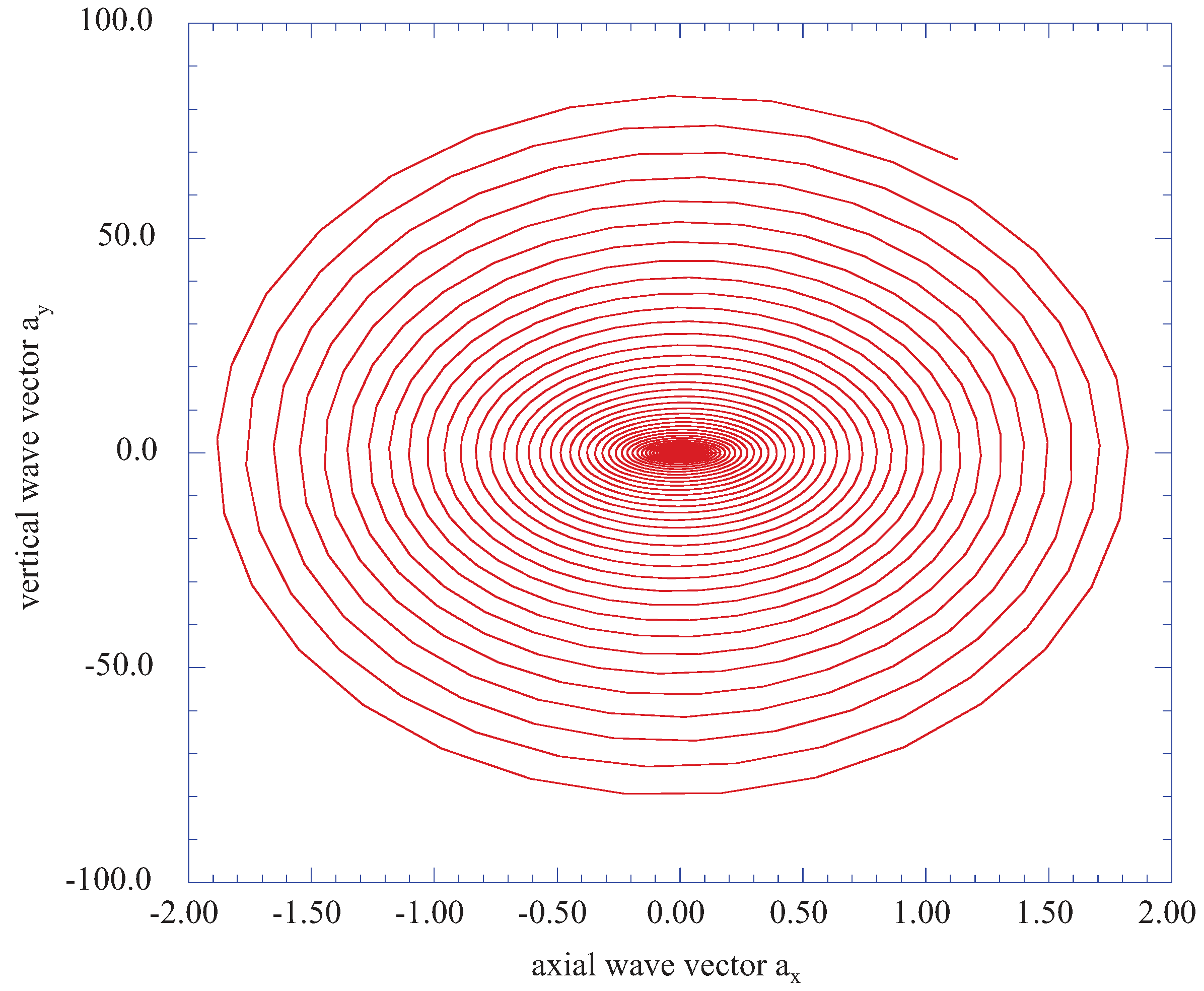
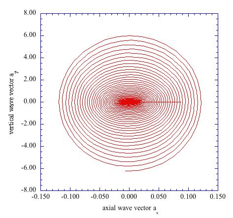
Figure 9 presents the phase plane plot of the vertical component of velocity wave vector, , versus the axial velocity wave vector component, , for the vertical location of j= 14 (η = 2.608).
Figure 9.
The phase plane representation of the vertical fluctuating velocity vector, against the horizontal fluctuating velocity vector, ax, at the vertical location of j = 14 (η = 2.608).
Figure 9.
The phase plane representation of the vertical fluctuating velocity vector, against the horizontal fluctuating velocity vector, ax, at the vertical location of j = 14 (η = 2.608).

These result are at the axial location of nx = 4 (x = 0.08). The phase components of the vertical and horizontal fluctuations have contracted significantly in a very short vertical direction. These results, however, imply the existence of a span wise vortex, with a significant rotation in the x-y plane for the velocity vectors. The prediction of a vertical “burst” of an ordered structure is evident in these results.
Figure 10 presents the time step results for the axial velocity wave vector component, ax, at the vertical station j = 18 (η = 3.414) and indicates the development of a weak instability in the wave vector results. These results are considerably reduced in value, thus indicating that at this further distance from the surface, the instabilities have decreased significantly.
Figure 11 is the phase plane plot of the vertical velocity wave vector, ay versus the axial velocity wave vector, ax for j = 18 (η=3.414), again demonstrating the reduced level of the instability.
Figure 10.
The axial velocity wave vector, ax, as a function of time step at the transformed vertical station of j = 18 (η= 3.414).
Figure 10.
The axial velocity wave vector, ax, as a function of time step at the transformed vertical station of j = 18 (η= 3.414).
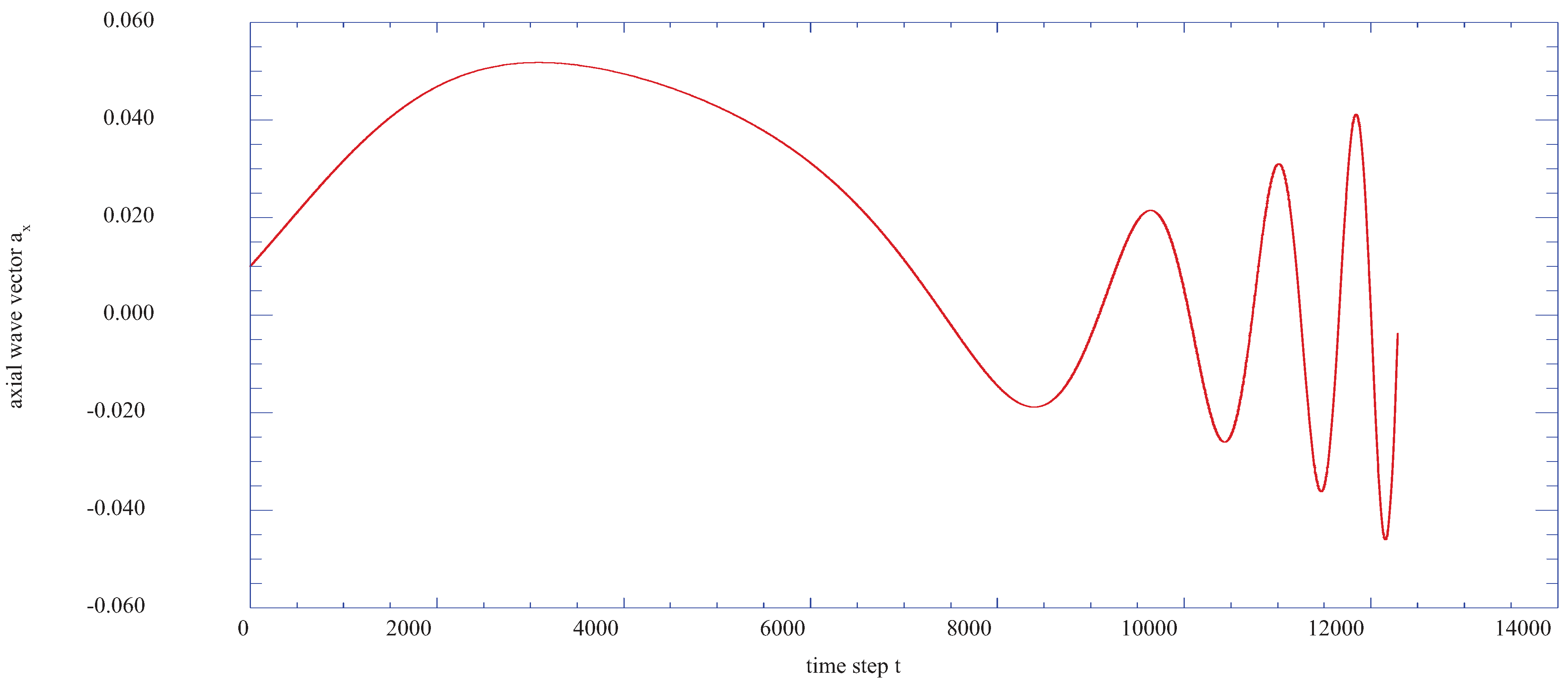
Figure 11.
The phase plane representation of the vertical velocity ay, versus the horizontal velocity ax, at the transformed vertical station of j = 18 (η= 3.414).
Figure 11.
The phase plane representation of the vertical velocity ay, versus the horizontal velocity ax, at the transformed vertical station of j = 18 (η= 3.414).
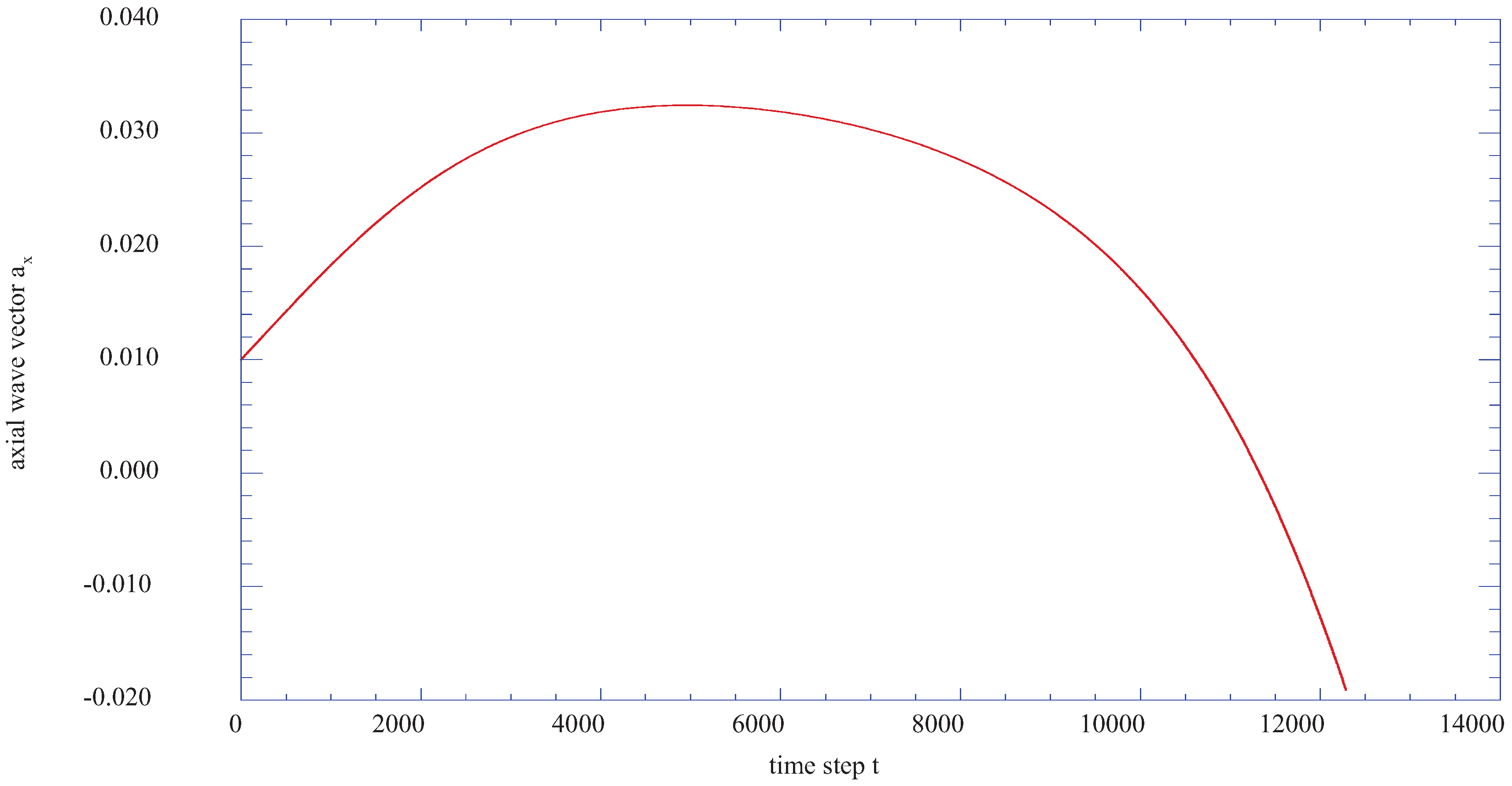
Finally, Figure 12 shows the time step results for the axial velocity wave vector, ax at the vertical station j = 22 (η = 4.221) indicating that at this station, the axial velocity wave vector changes direction from positive x to a negative x direction.
Figure 12.
The axial velocity wave vector, ax, as a function of time step at the transformed vertical station of j = 22 (η= 4.221).
Figure 12.
The axial velocity wave vector, ax, as a function of time step at the transformed vertical station of j = 22 (η= 4.221).
3.2. The Prediction of Spectral Entropy from the Deterministic Results
The Maximum Entropy Method (MEM) [41] is used extensively in the analysis of nonlinear time series data. Our use of this method is based upon the presentation by Chen [42], in which the method, known as Burg’s method, was applied to the extraction of spectral energy densities from seismic nonlinear time series data. Chen [42] presented the first source code for the improvement of Burg’s method in the extraction of the desired spectral information from the data.
One of the significant advantages of the maximum entropy method over the use of the filtered fast Fourier transform (FFT) method is the enhancement of the spectral peaks in the spectral energy density distribution. Our previous experience with the maximum entropy method and the existence of useful source codes for the analysis of the predicted time series led to our use of this method for the evaluation of the spectral entropy for each segment in the series of segments representing an internal block of data from the complete nonlinear time series data.
The method of analysis used for our study is the prediction of the distribution of the spectral entropy of the block of data in the computed nonlinear time series. The individual fluctuating histories for the axial and vertical velocity wave-vector components are combined into one time series by adding the squares of each component for each time step. The selected time series is divided into 64 segments with 32 data sets per segment. The maximum entropy method [41], is then applied to each segment of 32 data sets to obtain 16 spiked values of the power spectral density, fr, for each particular segment. The probability values of each set of particular spectral densities for each segment is then computed from . The methods of [43,44,45] are then applied to the probability distributions for each segment to develop the spectral entropy for the given segment. The spectral entropy (dimensionless) is defined as:
for the j-th segment. This procedure is applied to each of the 64 segments over the selected time range.
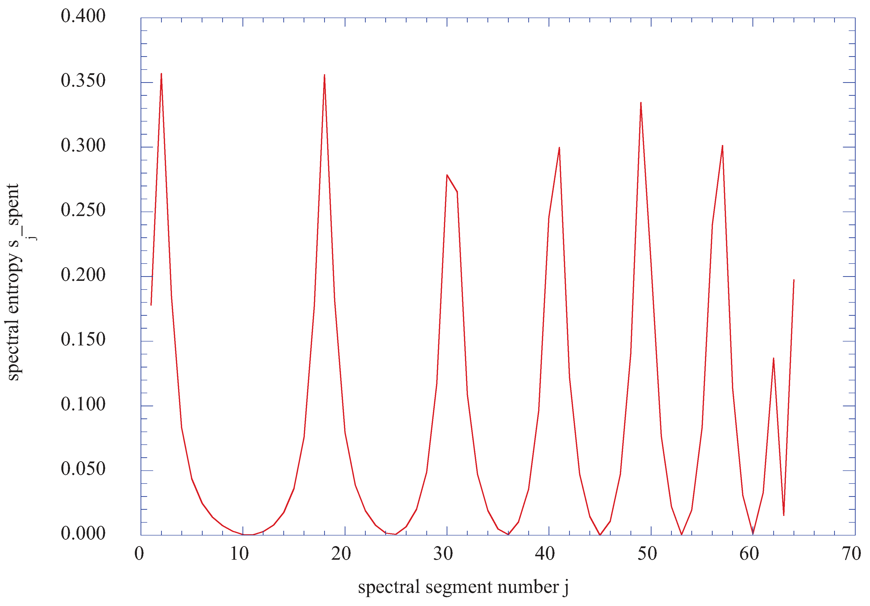
To establish an appropriate form for the set of equations describing the boundary-layer flow, we employed the following procedure: First, the physics of the shear layer are represented in the form of six first-order differential equations. The first three equations represent the evaluation of the behavior of the wave numbers with the imposed set of external control parameters throughout the integration process. Second, the integration of the equations of motion and the computation of the kinetic energy associated with the axial and vertical velocity fluctuations are computed. These are computed with the boundary layer velocity gradients serving as the set of internally applied control parameters. Third, local spectral entropy is computed for the vertical station of j = 16 (η = 3.011) at nx = 4 (x = 0.08) for the block of data from 8192 to 10240 time steps in the time span of the computation. Figure 13 indicates that for the selected time span, regions of sharp incoherent spectral entropy occur between broader regions of coherent spectral entropy. Low values of spectral entropy indicate coherent or ordered vortices, while high spectral entropy values indicate the dissolution of the ordered kinetic energy into regions of incoherent, but significant, kinetic energy. Figure 14, at j = 20 (η = 3.817), shows only a single peak of spectral entropy in a region of small spectral entropy, thus indicating a sharp region of dissolution of directed kinetic energy.
Figure 13.
The spectral entropy of ax2 + ay2 over 2048 time steps from the time step of 8192 to a time step of 10240 for the vertical location of j = 16 (η = 3.011) at nx = 4 (x = 0.08).
Figure 13.
The spectral entropy of ax2 + ay2 over 2048 time steps from the time step of 8192 to a time step of 10240 for the vertical location of j = 16 (η = 3.011) at nx = 4 (x = 0.08).

Figure 14.
The spectral entropy of ax2 + ay2 over 2048 time steps from the time step of 8192 to a time step of 10240 for the vertical location of j = 20 (η = 3.817) at nx = 4 (x = 0.08).
Figure 14.
The spectral entropy of ax2 + ay2 over 2048 time steps from the time step of 8192 to a time step of 10240 for the vertical location of j = 20 (η = 3.817) at nx = 4 (x = 0.08).
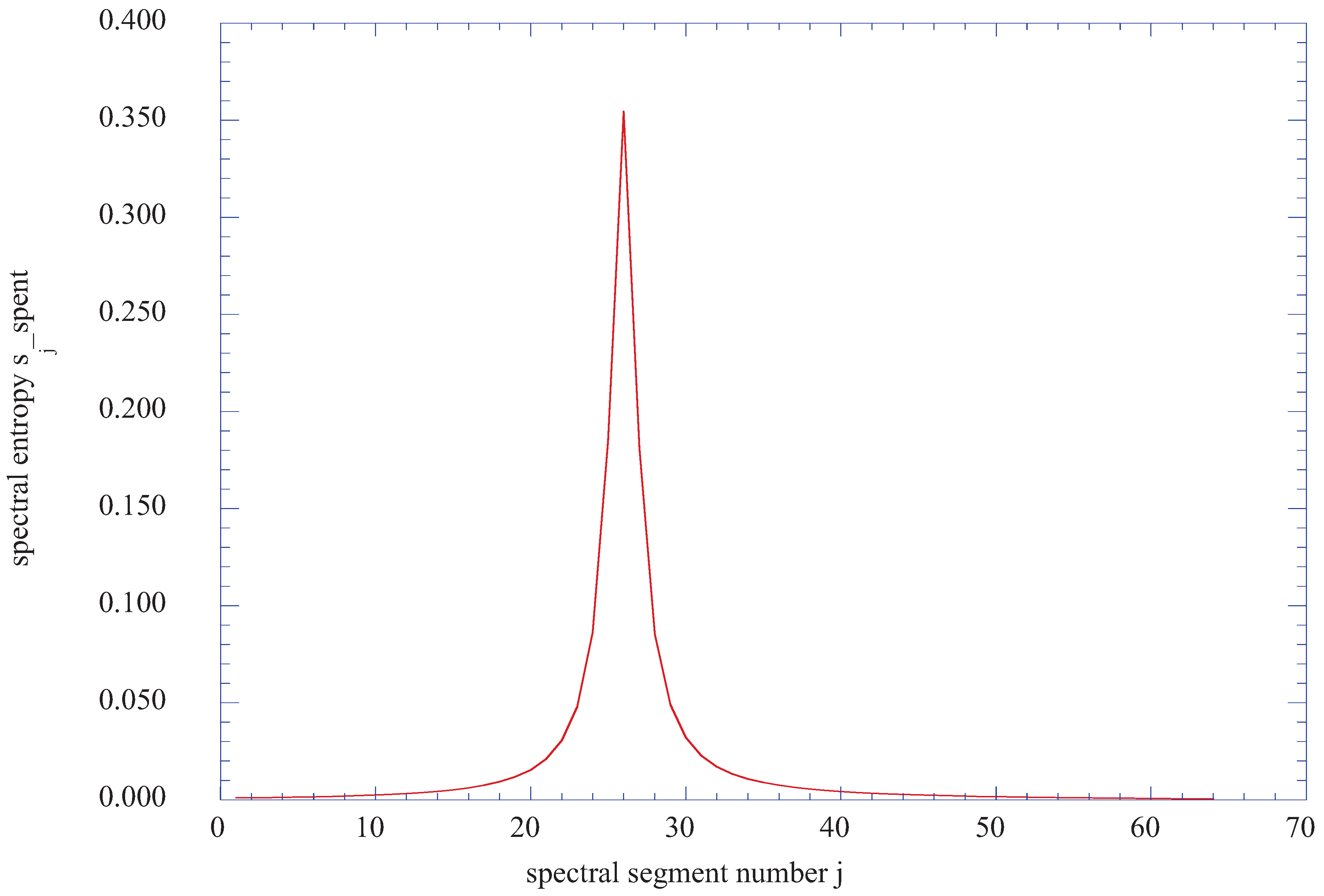
Figure 15 presents the spectral entropy for the vertical station of j = 22 (η = 4.221) at the axial station of nix = 4 (x = 0.08). Here, the spectral entropy does not indicate any peaks or valleys, but a uniformly increasing value across the selected time series. However, these values are three orders of magnitude smaller than the values indicated in the previous peaks of spectral entropy. Also, the dissolution of the instabilities into lower levels of spectral entropy occurs at just over half the height of the boundary layer thickness (η = 4.221 compared with ).
The region of spectral entropy values at j = 22 (η = 4.221) is the region that contributes to the predicted spectral entropy of the overall flow into the boundary-layer dissolution region. This region thus provides a source of flow element kinetic energy available for “dissolution” where the incoming spectral entropy flow is transformed into the wall thermodynamic entropy production region. These incoming flow elements thus provide a flow reservoir of spectral entropy elements, which, through an irrotational “scrambling” process, reach the level of physical scales that ultimately dissipate into background thermodynamic entropy [46]. Mathieu and Scott [47] have discussed this “scrambling” process in much more detail. Sagaut and Camdon [48] have described the flow of spectral entropy elements into the dissipation region as a “streaming” process.
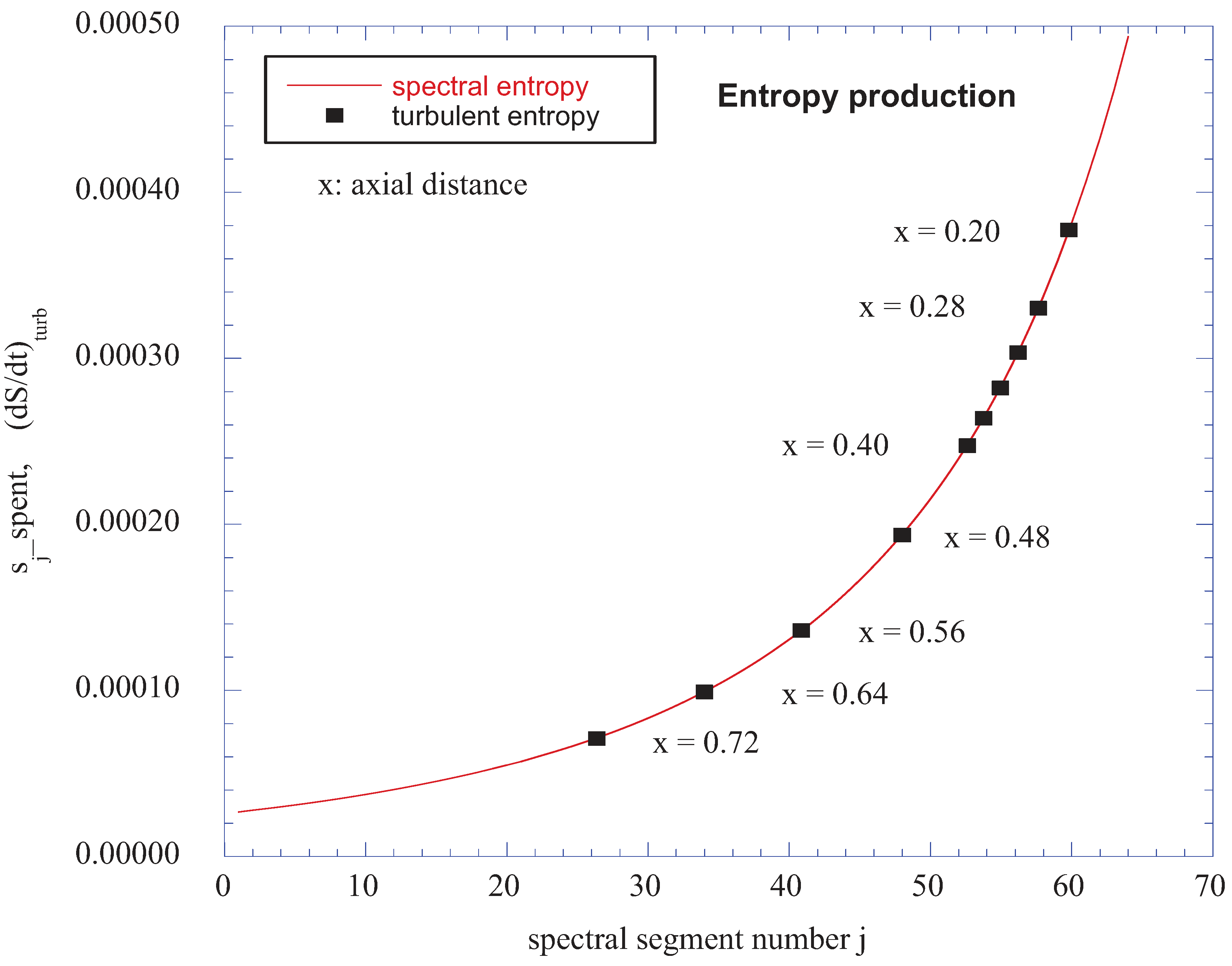
Figure 15 also shows selected maximum turbulent boundary layer entropy production rates for various axial positions along the shear layer. Note that the higher production rates are nearer the origin of the transition region, and decrease in maximum value along the axial distance of the wall shear layer.
Figure 15.
Comparison of wall shear layer maximum entropy production rates at various axial stations with values of spectral entropy of ax2 + ay2 for the vertical location of j = 22 (η = 4.221).
Figure 15.
Comparison of wall shear layer maximum entropy production rates at various axial stations with values of spectral entropy of ax2 + ay2 for the vertical location of j = 22 (η = 4.221).
4. Spectral Entropy Transfer Process
The primary objective of this study has been to obtain computed rates of entropy production in a physical flow environment using well-established numerical techniques, and to then explore an ad hoc flow instability within that physical environment for spectral entropies of comparable value. We should note that we have not established a rational connection between the computed values for each of the entropy parameters. The scientific connection between these two entropy concepts remains to be developed. In this section, we wish to explore a possible transfer mechanism for the spectral entropy to the wall layer for processing into thermodynamic entropy.
The entropy production results from the computational study of the boundary layer flow as distributed along the axial distance, x, are very close in value to the spectral entropy results found at the vertical station j = 22 (η = 4.221), above the unstable region of the boundary-layer profile.
Chow [8] has presented a computational procedure for evaluating the roll-up of wing-tip vortices produced by a lifting airfoil. In this procedure, a wing of total span of 2b is assumed to produce an axially directed vortex sheet from wing tip to wing tip. Chow [8] computes the induced vortex motion at the wing tip on one side of the total wingspan as a function of time from the initiation of the motion of the wing. This is accomplished by replacing the vortex sheet by a finite number of axially-directed spiral vortices and, from the law of Biot and Savart [8], determining the motion of the tip vortex induced by the finite number of vortices making up the vortex sheet.
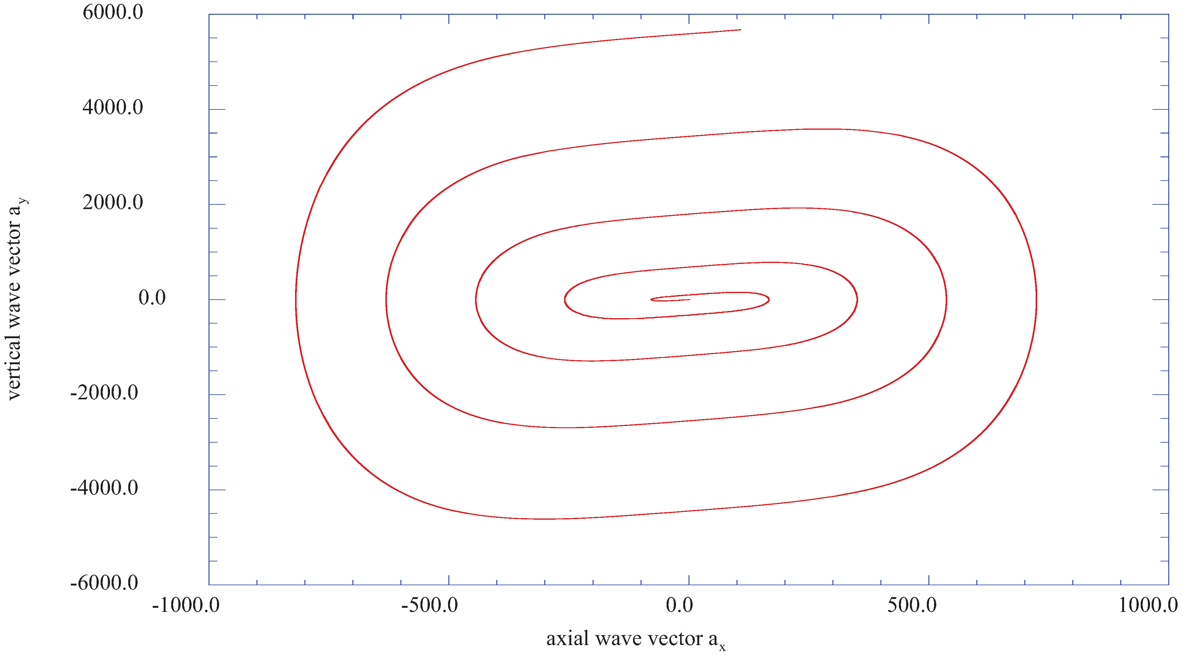
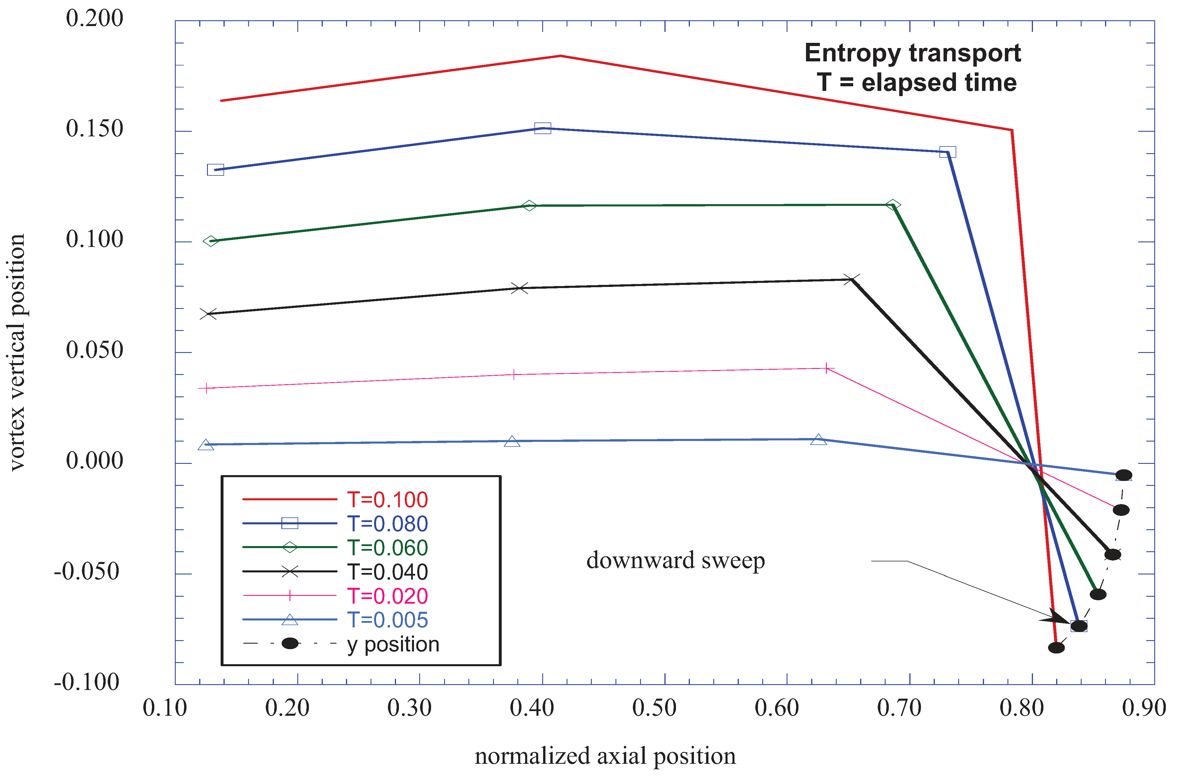
We have implemented this program to determine the motion of the upper part of the boundary-layer structure at j = 22 (η = 4.221) transporting the spectral elements into the wall shear layer. We assume the vortices in the unstable part of the vertical profile have axes in the z-direction, of unspecified span wise dimension. We then construct a vortex sheet with axes in the span wise direction between the original vortex axial location and an appropriate downstream axial station. We assume this distance to be normalized. We replace this vortex sheet with four span wise vortex structures, and use the program of [8] to compute the motion of the fourth structure. However, we invert the solution about the axial coordinate, with the results indicating the downward sweep of the induced vortex toward the wall shear layer. Figure 16 indicates the downward sweep of the induced vortex motion toward the wall shear layer. It should be noted that in Figure 16, the y position of y = 0.0 is the normalized vertical location of the original vortex structure and that the induced downward sweep is at a normalized axial station and is well below the vertical location of the original vortex.
If it is assumed that this entire process is reversible, then this mechanism brings those fluid elements represented by spectral entropy (or directed kinetic energy available for dissolution into thermodynamic entropy) into the wall shear layer for processing into thermodynamic entropy. Thus, the process of induced vortex motion and the concepts of intermittency and eddy viscosity seem to be closely related.
Figure 16.
Downward sweep of vortex motion induced by vortex instabilities in the upstream laminar boundary-layer velocity profile.
Figure 16.
Downward sweep of vortex motion induced by vortex instabilities in the upstream laminar boundary-layer velocity profile.
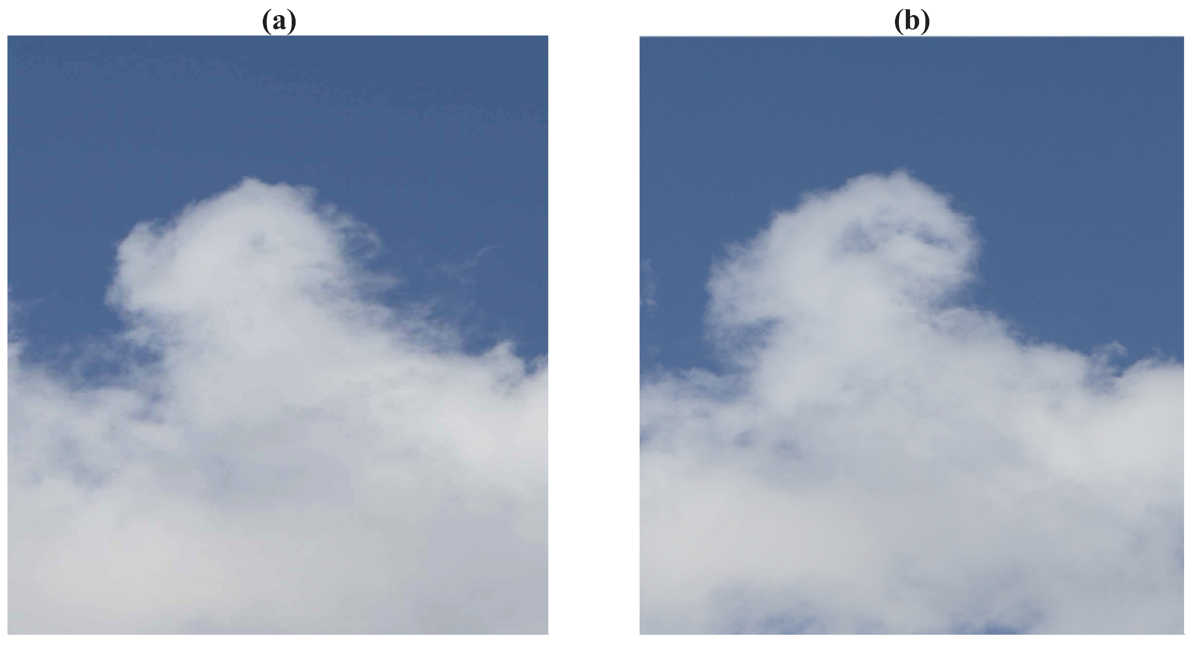
The establishment of a scientific relationship between spectral entropy and thermodynamic entropy will require the discovery of particular examples in which both parameters may be evaluated and connected with rational mathematical models. Photographs of the dynamic motion of the shear layer behavior above a cloud formation may be helpful in this regard.
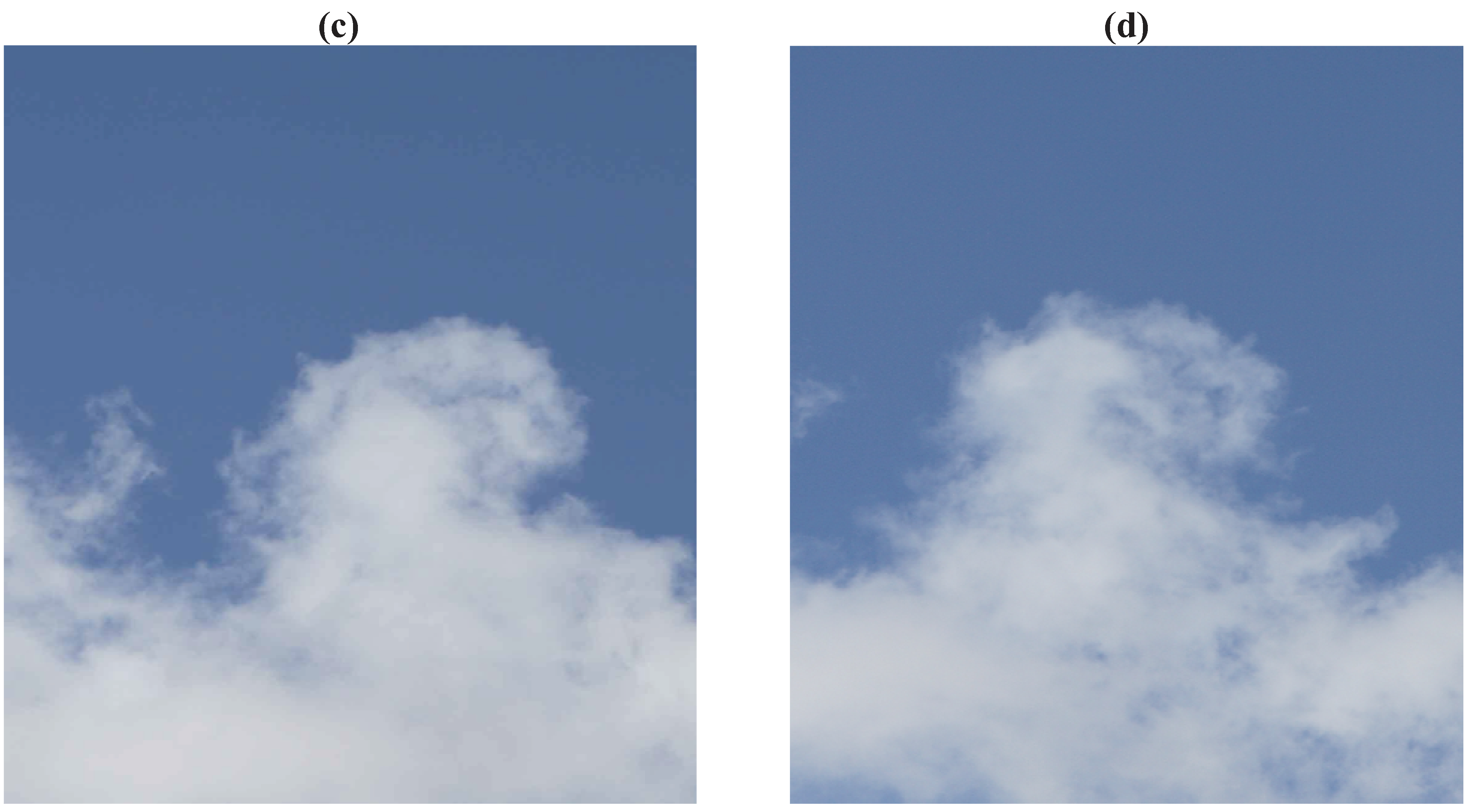
A sequence of photographs of the formation of instabilities along the vertical shear layer above a cumulus cloud structure is shown in Figure 17a–d. The atmospheric flow is from left to right. These photographs show the time development of an induced down sweep of the upper layers of the vortex structure. If it assumed that the flow elements with the highest spectral entropy are along the top layer of the induced flow, then these photographs indicate that the upper layer is transported deepest toward the origin of the instability. This is in agreement with the computations of the axial distribution of the shear layer entropy, with the highest shear layer entropy production rate at the axial distance of nx = 10 (x = 0.20), decreasing to the lowest calculated value at nx = 36 (x = 0.72). Thus, the induced down sweep of the vortex structure may spread the spectral elements along the axial distance, in an inverse manner relative to the values of the spectral entropy. The final image indicates that the down sweep structure then uniformly dissolves into the background flow.
Figure 17.
(a) Photograph of a spiral vortex formed in the vertical shear layer above a cumulus cloud. The atmospheric flow is from left to right. (b) The induced down sweep of the vortex motion. (c) The upper surface of the induced down sweep moves deepest toward the origin. (d) Dissolution of the down sweep structure.

5. Conclusions
The complete set of equations for the fluctuating velocity wave vectors within a boundary-layer flow has been reduced to a set of equations similar to the Lorenz equations with the introduction of sets of external and internal control parameters. It should be noted that the computed values for the spectral entropy for each of the vertical boundary layer locations is the spectral entropy of the squared values of the fluctuating axial and vertical velocity wave-vectors. The occurrence of a strong vertical “burst” of instability is found near the surface of the boundary-layer flow and that the instability propagates vertically into the shear layer. It has also been found that the intensity of the alternating coherent and incoherent portions of the instability decrease in the vertical direction of the boundary layer profile. At a certain position within the vertical velocity profile, the instability has transformed into a completely incoherent form with a spectral entropy distribution that inversely mirrors the development of the entropy production rate along the axial direction of the transitional boundary-layer flow. The fluid element instability behavior undergoes a “streaming” or a “dissolution” into the range of ultimate dissipation of the turbulent kinetic energy into background thermodynamic entropy within the region near the wall in the shear layer flow. The results for the numerical calculations of spectral entropy distribution across the shear layer show very close inverse agreement with the computationally determined entropy production rate in the transitional wall shear layer for various axial positions along the wall.
Nomenclature
| ai | Fluctuating i-th component of velocity wave vector |
| b | Eddy viscosity function in transformed boundary layer equation |
| f | Dimensionless stream function |
| f’ | First derivative of f with respect to η |
| f’’ | Second derivative of f with respect to η |
| fr | Sum of the squares of the fluctuating axial and vertical velocity wave vectors |
| F1 | Time-dependent perturbation factor |
| j | Vertical station number in the boundary layer computations |
| j | Spectral entropy segment number |
| k | Time-dependent wave number vector |
| ki | Fluctuating i-th wave number of Fourier expansion |
| K1 | Adjustable weight factor |
| m | Pressure gradient parameter |
| M | Molecular weight |
| nx | Axial station number in the boundary layer computations |
| p | Hydrostatic pressure |
| Pr | Power spectral density of the r-th spectral segment |
| P0 | Boundary layer edge pressure |
| R | Appropriate gas constant |
| sj_spent | Spectral entropy for the j-th time series data segment |
Rate of dimensionless entropy production (1/s) in the shear layer | |
Rate of volumetric entropy production in the shear layer | |
Rate of dimensionless entropy production (1/s) in the turbulent boundary layer | |
| t | Time |
| T | Static temperature |
| T0 | Boundary layer edge temperature |
| u | Axial boundary layer velocity |
| u’ | Axial boundary layer fluctuation velocity |
| ue | Axial velocity at the outer edge of the boundary layer |
| ui | Fluctuating i-component of velocity instability |
| Ui | Mean velocity in the i-direction |
| v | Vertical boundary layer velocity |
| v’ | Vertical boundary layer fluctuation velocity |
| Vy | Mean vertical velocity in the x-y plane |
| Vz | Mean vertical velocity in the y-z plane |
| w | Span wise boundary layer velocity |
| W | Mean velocity in the span wise direction |
| x | Axial direction |
| xi | i-th direction |
| xj | j-th direction |
| y | Vertical direction |
| z | Span wise direction |
Greek Letters
| δ | Boundary layer thickness |
| εm | Eddy viscosity |
| εm+ | Dimensionless eddy viscosity |
| η | Normalized vertical distance |
| μ | Dynamic viscosity |
| ρ | Density |
Kinematic viscosity | |
| ω | External control parameter, frequency factor |
| Ψ | Transformed stream function |
Subscripts
| i, j, l, m | Tensor indices |
| r | The r-th index in the j-th time series data segment |
| 0 | Stagnation state, reference value |
| x | Component in the x-direction |
| y | Component in the y-direction |
| z | Component in the z-direction |
Acknowledgements
The author would like to thank the editors and referees for their timely and insightful suggestions. Incorporation of these suggestions has been particularly helpful in the presentation.
References
- Cebeci, T.; Bradshaw, P. Momentum Transfer in Boundary Layers; Hemisphere: Washington, DC, USA, 1977. [Google Scholar]
- Cebeci, T.; Bradshaw, P. Physical and Computational Aspects of Convective Heat Transfer; Springer-Verlag: New York, NY, USA, 1984. [Google Scholar]
- Cebeci, T. Convective Heat Transfer; Springer-Verlag: New York, NY, USA, 2002. [Google Scholar]
- Cebeci, T.; Cousteix, J. Modeling and Computation of Boundary-Layer Flows, 2nd ed.; Horizons: Long Beach, CA, USA, 2005. [Google Scholar]
- Townsend, A.A. The Structure of Turbulent Shear Flow, 2nd ed.; Cambridge University Press: Cambridge, UK, 1976; pp. 45–49. [Google Scholar]
- Isaacson, L.K. A deterministic prediction of ordered structures in an internal free shear layer. J. Non-Equilib. Thermodyn. 1993, 18, 256–270. [Google Scholar] [CrossRef]
- Isaacson, L.K. Deterministic Prediction of the Entropy Increase in a Sudden Expansion. Entropy 2011, 13, 402–421. [Google Scholar] [CrossRef]
- Chow, C.Y. An Introduction to Computational Fluid Mechanics; Seminole Pub. Co.: Boulder, CO, USA, 1983; pp. 309–322. [Google Scholar]
- Hansen, A.G. Similarity Analyses of Boundary Value Problems in Engineering; Prentice-Hall, Inc.: Englewood Cliffs, NJ, USA, 1964; pp. 86–92. [Google Scholar]
- Zucrow, M.J.; Hoffman, J.D. Gas Dynamics; John Wiley & Sons, Inc.: New York, NY, USA, 1976; Volume I, pp. 20–23. [Google Scholar]
- Schlichting, H. Boundary-Layer Theory, 7th ed.; McGraw-Hill Book Company: New York, NY, USA, 1979; pp. 265–268. [Google Scholar]
- Bird, R.B.; Stewart, W.E.; Lightfoot, E.N. Transport Phenomena; John Wiley & Sons: New York, NY, USA, 1960. [Google Scholar]
- Truitt, R.W. Fundamentals of Aerodynamic Heating; Ronald Press Company: New York, NY, USA, 1960; pp. 9–20. [Google Scholar]
- Bejan, A. Entropy Generation Minimization; CRC Press, Inc.: Boca Raton, FL, USA, 1996; pp. 47–59. [Google Scholar]
- Longwell, P. A. Mechanics of Fluid Flow; McGraw-Hill Book Company: New York, NY, USA, 1966; pp. 336–342. [Google Scholar]
- Landau, L.D.; Lifshitz, E.M. Statistical Physics; Pergamon Press LTD: London, UK, 1958; pp. 28–31. [Google Scholar]
- Sonntag, R.E.; Van Wylen, G.J. Fundamentals of Statistical Thermodynamics; Robert E. Krieger Pub. Co., Inc.: Malabar, FL, USA, 1985; p. 117. [Google Scholar]
- Glansdorff, P.; Prigogine, I. Thermodynamic Theory of Structure, Stability and Fluctuations; John Wiley & Sons Ltd.: London, UK, 1971. [Google Scholar]
- Chapman, S.; Cowling, T.G. The Mathematical Theory of Non-Uniform Gases, 3rd ed.; Cambridge: London, UK, 1970; pp. 97–131. [Google Scholar]
- Vincenti, W.G.; Kruger, C.H., Jr. Introduction to Physical Gas Dynamics; John Wiley & Sons, Inc.: New York, NY, USA, 1965; pp. 384–412. [Google Scholar]
- Schlichting, H. Boundary-Layer Theory, 7th ed.; McGraw-Hill Book Company: New York, NY, USA, 1979; pp. 451–452. [Google Scholar]
- Schlichting, H. Boundary-Layer Theory, 7th ed.; McGraw-Hill Book Company: New York, NY, USA, 1979; pp. 578–593. [Google Scholar]
- Cebeci, T.; Smith, A.M.O. Analysis of Turbulent Boundary Layers; Academic Press: New York, NY, USA, 1974; pp. 234–239. [Google Scholar]
- Klimontovich, Y.L. Statistical Physics; Harwood Academic Publishers: London, UK, 1986; pp. 686–689. [Google Scholar]
- Ebeling, W. On the entropy of dissipative and turbulent structures. Physica Scripta. 1989, T25, 238–242. [Google Scholar] [CrossRef]
- Engel-Herbert, H.; Ebeling, W. The behavior of the entropy during transitions from thermodynamic equilibrium. II. Hydrodynamic flows. Physica 1988, 149A, 195–205. [Google Scholar] [CrossRef]
- Crepeau, J.C. Spectral Entropy Behavior in Transitional Flows. PhD Dissertation, Department of Mechanical Engineering, University of Utah, Salt Lake City, UT, USA, June 1991. [Google Scholar]
- Gad-el-Hak, M.; Tsai, H.M. Transition and Turbulence Control; World Scientific Pub. Co.: Singapore, 2006. [Google Scholar]
- Andersson, P.; Berggren, M.; Henningson, D.S. Optimal disturbances and bypass transition in boundary layers. Phys. Fluids 1999, 11, 134–150. [Google Scholar] [CrossRef]
- Corbett, P.; Bottaro, A. Optimal perturbations for boundary layers subject to stream-wise pressure gradient. Phys. Fluids 2000, 12, 120–130. [Google Scholar] [CrossRef]
- Brandt, L.; de Lange, H.C. Streak interactions and breakdown in boundary layer flows. Phys. Fluids 2008, 20. [Google Scholar] [CrossRef]
- Hoepffner, J.; Brandt, L. Stochastic approach to the receptivity problem applied to bypass transition in boundary layers. Phys. Fluids 2008, 20. [Google Scholar] [CrossRef]
- Schlatter, P.; Brandt, L.; de Lange, H.C.; Henningson, D.S. On streak breakdown in bypass transition. Phys. Fluids 2008, 20. [Google Scholar] [CrossRef]
- Landau, L.D.; Lifshitz, E.M. Quantum Mechanics: Non-Relativistic Theory; Pergamon Press, Ltd.: London, UK, 1958; pp. 133–144. [Google Scholar]
- Hellberg, C.S.; Orszag, S.A. Chaotic behavior of interacting elliptical instability modes. Phys. Fluid. 1988, 31, 6–8. [Google Scholar] [CrossRef]
- Klimontovich, Y.L.; Bonitz, M. Definition of the degree of order in selforganization processes. Annalen der Physik. 1988, 7, 340–352. [Google Scholar] [CrossRef]
- Pyragas, K. Continuous control of chaos by self-controlling feedback. Phys. Lett. A 1990, 170, 421–427. [Google Scholar] [CrossRef]
- Pyragas, K. Predictable chaos in slightly perturbed unpredictable chaotic systems. Phys. Lett. A 1993, 181, 203–210. [Google Scholar] [CrossRef]
- Press, W.; Teukolsky, S.A.; Vetterling, W.T.; Flannery, B.P. Numerical Recipes in C: The Art of Scientific Computing, 2nd ed.; Cambridge University Press: Cambridge, UK, 1992; pp. 710–714. [Google Scholar]
- Press, W.; Teukolsky, S.A.; Vetterling, W.T.; Flannery, B.P. Numerical Recipes in C: The Art of Scientific Computing, 2nd ed.; Cambridge University Press: Cambridge, UK, 1992; pp. 572–575. [Google Scholar]
- Chen, C.H. Digital Waveform Processing and Recognition; CRC Press, Inc.: Boca Raton, FL, USA, 1982; pp. 131–158. [Google Scholar]
- Powell, G.E.; Percival, I.C. A spectral entropy method for distinguishing regular and irregular motion for Hamiltonian systems. J. Phys. Math. Gen. 1979, 12, 2053–2071. [Google Scholar] [CrossRef]
- Grassberger, P.; Procaccia, I. Estimation of the Kolmogorov entropy from a chaotic signal. Phys. Rev. A 1983, 28, 2591–2593. [Google Scholar] [CrossRef]
- Cohen, A.; Procaccia, I. Computing the Kolmogorov entropy from time signals of dissipative and conservative dynamical systems. Phys. Rev. A 1985, 31, 1872–1882. [Google Scholar] [CrossRef] [PubMed]
- Hinze, J.O. Turbulence, 2nd ed.; McGraw-Hill, Inc.: New York: NY, USA, 1975; pp. 684–690. [Google Scholar]
- Mathieu, J.; Scott, J. An Introduction to Turbulent Flow; Cambridge University Press: Cambridge, UK, 2000; p. 299. [Google Scholar]
- Sagaut, P.; Cambon, C. Homogeneous Turbulence Dynamics; Cambridge University Press: New York, NY, USA, 2008; p. 75. [Google Scholar]
© 2011 by the authors; licensee MDPI, Basel, Switzerland. This article is an open access article distributed under the terms and conditions of the Creative Commons Attribution license (http://creativecommons.org/licenses/by/3.0/).
Share and Cite
MDPI and ACS Style
Isaacson, L.K. Spectral Entropy in a Boundary-Layer Flow. Entropy 2011, 13, 1555-1583. https://doi.org/10.3390/e13091555
AMA Style
Isaacson LK. Spectral Entropy in a Boundary-Layer Flow. Entropy. 2011; 13(9):1555-1583. https://doi.org/10.3390/e13091555
Chicago/Turabian StyleIsaacson, LaVar King. 2011. "Spectral Entropy in a Boundary-Layer Flow" Entropy 13, no. 9: 1555-1583. https://doi.org/10.3390/e13091555