Universal Property of Quantum Gravity implied by Uniqueness Theorem of Bekenstein-Hawking Entropy

Abstract
:1. Introduction
2. Uniqueness of Bekenstein-Hawking Entropy
2.1. Ordinary Thermodynamics in Axiomatic Formulation
2.1.1. Adiabatic Process and Composition
2.1.2. Basic Properties of State Variables
2.1.3. Entropy in Ordinary Thermodynamics
2.2. Black Hole Thermodynamics
2.2.1. Thermal Equilibrium of Schwarzschild Black Hole
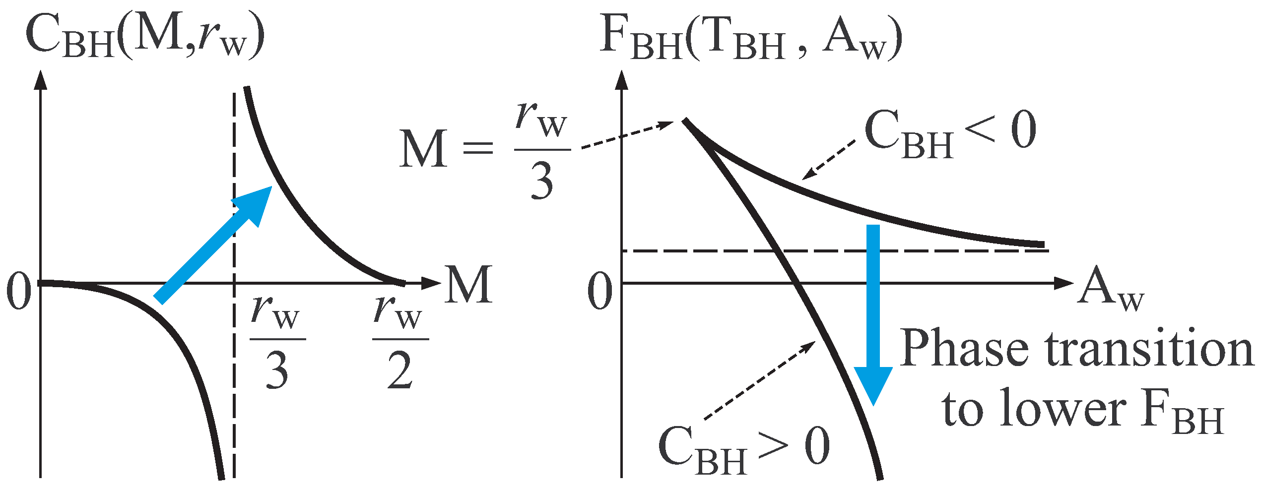
2.2.2. Thermal Stability of Schwarzschild Black Hole
2.2.3. Scaling Behavior of State Variables
- Extensive variable: These variables, X (e.g., , and ), are scaled as, .
- Intensive variable: These variables, Y (e.g., and ), are scaled as, .
- Thermodynamic energy: These energies, Z (e.g., and ), are scaled as, .
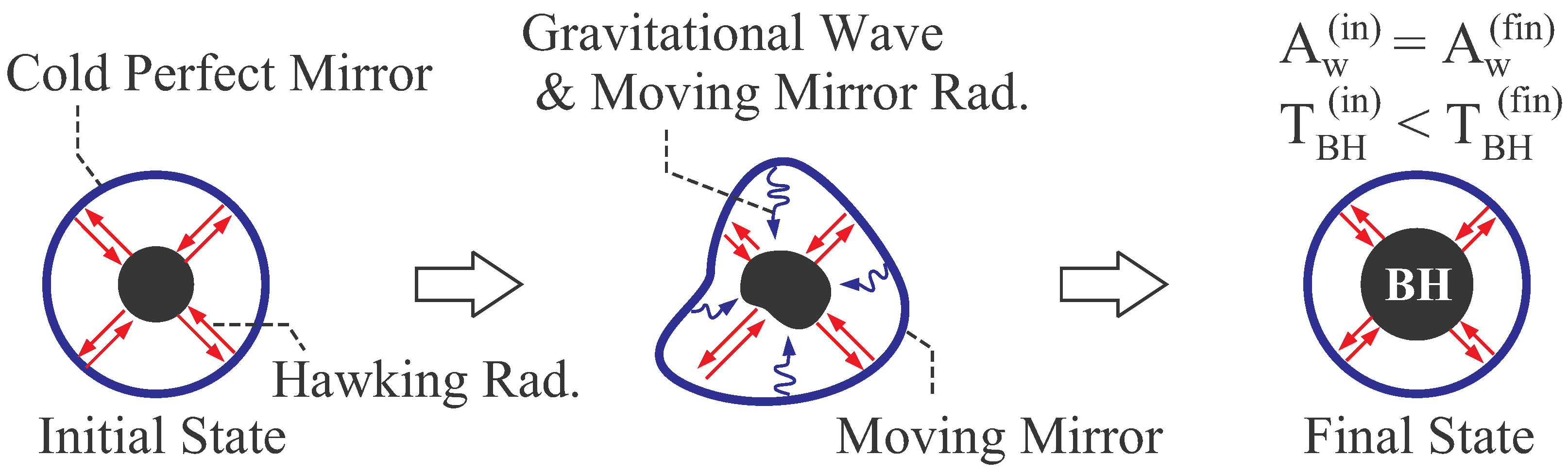
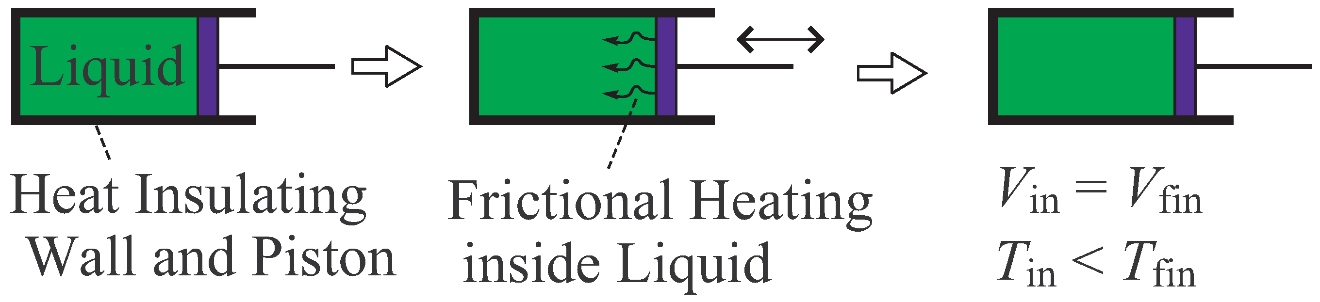
2.2.4. Adiabatic Process and Composition
2.2.5. Basic Properties of Bekenstein-Hawking Entropy
- Extensivity of formulated in Definition 3.
- Additivity of in Equation (18).
- Entropy principle shown in Fact 1. (See comments given below.)
- Uniqueness of . (Proof is given in the next subsection.)
- Concavity of about internal energy and system size . (Detail is given below.)
- Monotone increasing nature of about . (Detail is given below.)
2.3. Uniqueness Theorem of Bekenstein-Hawking Entropy
2.3.1. Statement of Theorem
2.3.2. Proof of Theorem 1 (preparations)
- Step 1:
- Show the positivity of .
- Step 2:
- Show that the relation, , holds with arbitrary X, where .
- Step 3:
- Show that the relation, , holds with arbitrary Y.
- Step 4:
- Show the extensivity of η.
2.3.3. Step 1 of the Proof
2.3.4. Step 2 of the Proof
2.3.5. Step 3 of the Proof
2.3.6. Step 4 of the Proof
3. Conditions Justifying Boltzmann formula
3.1. Statements of Theorems and a Corollary without Proof
- Condition A : Arbitrary j-particle interaction, , becomes negative for sufficiently large distribution of j particles. That is, there exists a constant , such that
- Condition B : The potential Φ is bounded below. That is, there exists a constant , such that
- Result 1 : The “large system limit” of the density of ground state energy exists,where is the eigen value of ground state defined in Equation (39), and means the large system limit defined by with fixing at a constant value. This limit, , is bounded below and determined uniquely.
- Result 2 : When does not diverge to , the “thermodynamic limit” of the logarithmic density of number of states exists,where means the thermodynamic limit defined by with fixing and at constant values. This limit, , is determined uniquely. Furthermore, is concave about its arguments , and monotone increasing about ε.
- Presupposition C : The j-particle interactions for disappear, and the total interaction potential Φ is a sum of two-particle interactions, .
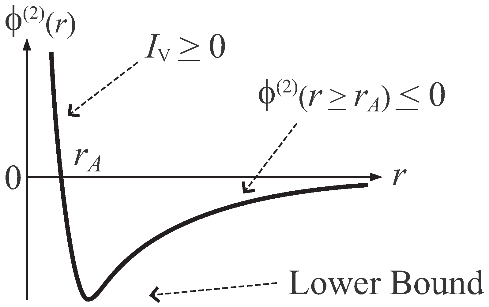
- Presupposition D : Introduce a differential quantity, , of potential Φ defined aswhere is the large system limit defined in Ruelle-Tasaki theorem, and (at least one Laplacian, , operates on Φ). Then, the presupposition D is the requirement that this quantity satisfies the relation,where γ is an arbitrary finite constant.
3.2. Proof of Dobrushin Theorem
4. Conclusion: Suggestion on Universal Property of Quantum Gravity
Acknowledgements
References and Notes
- Bardeen, J.M.; Carter, B.; Hawking, S.W. The four laws of black hole mechanics. Commun. Math. Phys. 1973, 31, 161–170. [Google Scholar] [CrossRef]
- Bekenstein, J.D. Black holes and entropy. Phys. Rev. 1973, D7, 2333–2346. [Google Scholar] [CrossRef]
- Bekenstein, J.D. Generalized second law of thermodynamics in black-hole physics. Phys. Rev. 1974, D9, 3292–3300. [Google Scholar] [CrossRef]
- Braden, H.W.; Brown, J.D.; Whiting, B.F.; York, J.W., Jr. Charged black hole in a grand canonical ensemble. Phys. Rev. 1990, D42, 3376–3385. [Google Scholar] [CrossRef]
- Brown, J.D.; Martinez, E.A.; York, J.W., Jr. Complex Kerr-Newman geometry and black-hole thermodynamics. Phys. Rev. Lett. 1991, 66, 2281–2284. [Google Scholar] [CrossRef] [PubMed]
- Davies, P.C.W. The thermodynamics theory of black holes. Proc. R. Soc. Lond. 1977, A353, 499–521. [Google Scholar] [CrossRef]
- Hawking, S.W. Gravitational radiation from colliding black holes. Phys. Rev. Lett. 1971, 26, 1344–1346. [Google Scholar] [CrossRef]
- Hawking, S.W. Particle creation by black holes. Commun. Math. Phys. 1975, 43, 199–220. [Google Scholar] [CrossRef]
- Israel, W. Third law of black-hole dynamics: A formulation and proof. Phys. Rev. Lett. 1986, 57, 397–399. [Google Scholar] [CrossRef] [PubMed]
- York, J.W., Jr. Black-hole thermodynamics and the Euclidean Einstein action. Phys. Rev. 1986, D33, 2092–2099. [Google Scholar] [CrossRef]
- Flanagan, E.E.; Marolf, D.; Wald, R.M. Proof of classical version of the Bousso entropy bound and of the generalized second law. Phys. Rev. 2000, D62, 084035:1–12. [Google Scholar] [CrossRef]
- Frolov, V.P.; Page, D.N. Proof of the generalized second law for quasistationary semiclassical black holes. Phys. Rev. Lett. 1993, 71, 3902–3905. [Google Scholar] [CrossRef] [PubMed]
- Saida, H. The generalized second law and the black hole evaporation in an empty space as a nonequilibrium process. Class. Quant. Grav. 2006, 23, 6227–6243. [Google Scholar] [CrossRef]
- Unruh, W.G.; Wald, R.M. Accelerated radiation and the generalized second law of thermodynamics. Phys. Rev. 1982, D25, 942–958, (Correction in Phys. Rev. 1988, D37, 3059–3060). [Google Scholar]
- Unruh, W.G.; Wald, R.M. Entropy bounds, acceleration radiation, and the generalized second law. Phys. Rev. 1983, D27, 2271–2276. [Google Scholar] [CrossRef]
- Saida, H. To what extent is the entropy-area law universal?—Multi-horizon and multi-temperature spacetime may break the entropy-area law. Prog. Theor. Phys. 2009, 122, 1515–1552. [Google Scholar] [CrossRef]
- Birrell, N.D.; Davies, P.C.W. Quantum fields in curved space; Cambridge Univ. Press: Cambridge, UK, 1982. [Google Scholar]
- Bousso, R. The holographic principle. Rev. Mod. Phys. 2002, 74, 825–874. [Google Scholar] [CrossRef]
- Lieb, E.H.; Yngvason, J. The physics and mathematics of the second law of thermodynamics. Phys. Rep. 1999, 310, 1–96. [Google Scholar] [CrossRef]
- Tasaki, H. Thermodynamics (Netsu-Rikigaku); Baifu-Kan Publ: Tokyo, Japan, 2000; (Published in Japanese). [Google Scholar]
- Dobrushin, R.L. Investigation of the conditions of the asymptotic existence of the configuration integral of the Gibbs distribution. Teor. Veroyatnost. i Primenen. 1964, 9, 626–643. [Google Scholar] [CrossRef]
- Ruelle, D. Statistical Mechanics: Rigorous Results; Imperial College Press and World Scientific Publ.: London and Singapore, UK and Singapore, 1999; Chapter 1–3. [Google Scholar]
- Tasaki, H. Statistical Mechanics (Tokei-Rikigaku); Baifu-Kan Publ.: Tokyo, Japan, 2008; (Published in Japanese). [Google Scholar]
- The increase of temperature by this adiabatic process is regarded as one basic principle in the axiomatic thermodynamics.
- For example, the Kelvin’s statement of second law, the basic principles mentioned in notes [24] and [26], and so on.
- One of basic principles of axiomatic thermodynamics is the existence of an adiabatic process which connects arbitrary two thermal equilibrium states. The “direction” of adiabatic process is to be determined by the entropy principle.
- The ratio of Hawking temperature, given in Equation (10) at spatial infinity (), to black hole mass energy, Mc2, is . This ratio is of order unity for Planck mass, g. For solar mass black hole, g, this ratio is of order 10−77.
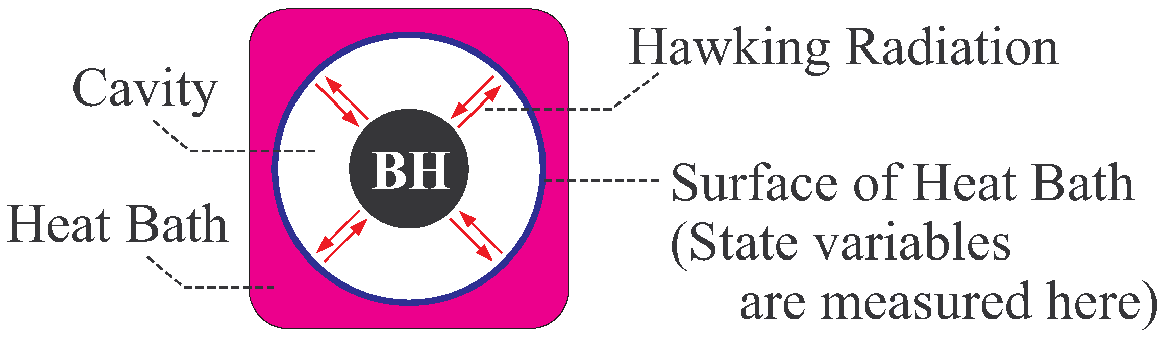
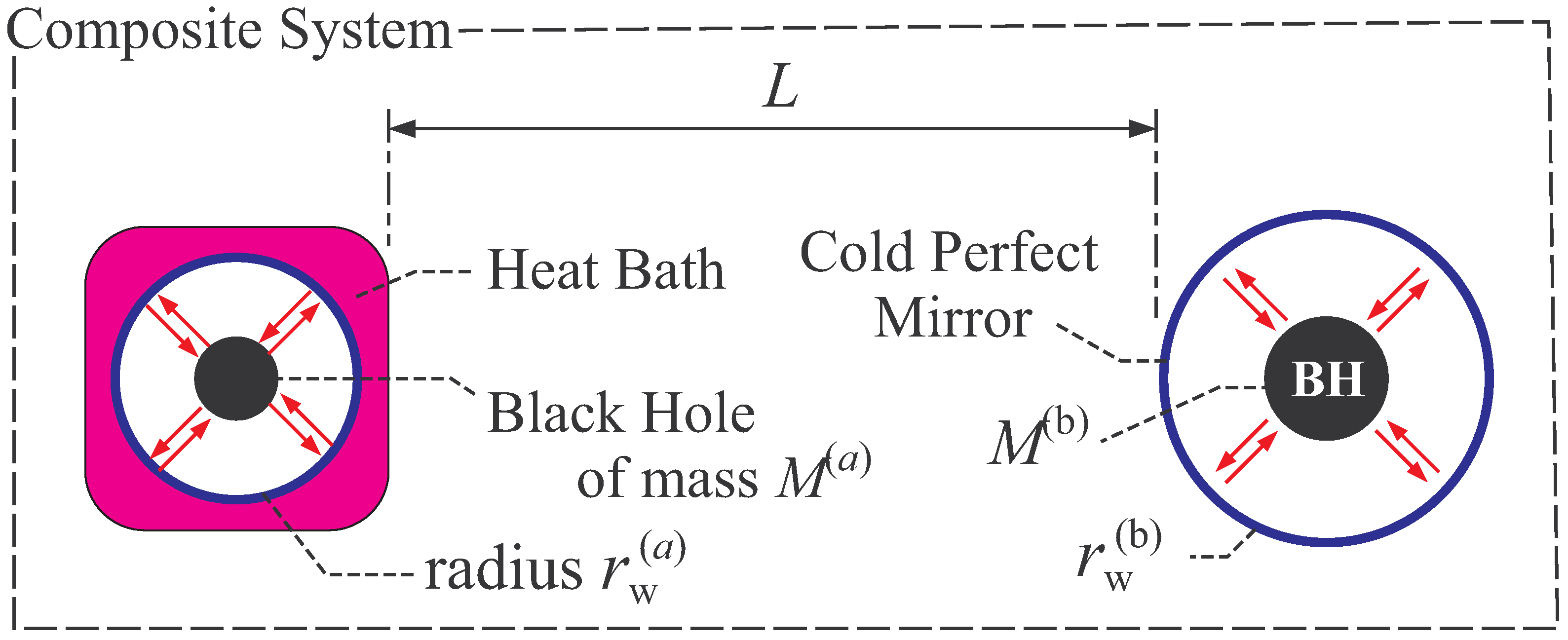
- In general, global thermal equilibrium state does not evolve in time by its definition. In black hole thermodynamics, we consider the global equilibrium of the system shown in Figure 2, and thus the static coordinate is suitable. Here, we should distinguish the “global” equilibrium and “local” equilibrium. For example, a fluid can be in local equilibrium, in which each fluid element is in a thermal equilibrium state but the equilibrium state of one fluid element is not necessarily the same with that of the other element. The fluid is globally in non-equilibrium states, since the states of fluid elements do not necessarily balance with each other. The fluid evolves in time due to this global non-equilibrium nature.
- Tolman, R.C. Relativity, Thermodynamics and Cosmology; Dover Publ.: New York, NY, USA, 1987; Chapter 9. [Google Scholar]
- Gibbons, G.W.; Hawking, S.W. Action integrals and partition functions in quantum gravity. Phys. Rev. 1977, D15, 2752–2256. [Google Scholar] [CrossRef]
- Hawking, S.W. The Path-integral approach to quantum gravity. In Euclidean Quantum Gravity; Gibbons, G.W., Hawking, S.W., Eds.; World Scientific Publ.: Singapore, 1993. [Google Scholar]
- Saida, H. de Sitter thermodynamics in the canonical ensemble. Prog. Theor. Phys. 2009, 122, 1239–1266. [Google Scholar] [CrossRef]
- Fulling, S.A.; Davies, P.C.W. Radiation from a moving mirror in two dimensional space-time: Conformal anomaly. Proc. R. Soc. Lond. 1976, A348, 393–414. [Google Scholar] [CrossRef]
- Martinez, E.A.; York, J.W., Jr. Additivity of the entropies of black holes and matter in equilibrium. Phys. Rev. 1989, D40, 2124–2127. [Google Scholar] [CrossRef]
- One may consider, for example, the electron gas as an example of the system which violates the Condition A but retains the Boltzmann formula, since the interaction potential between electrons is positive at large distances and violates the Condition A. However let us note that, in Ruelle’s book [22], the Condition A is extended so as to include the interaction potential which can become positive and repulsive at large distances. (Note that it is sufficient for the aim of this paper to consider the case that the potential is negative at large distances, such as the Newtonian gravity.) Hence, by such an extension of Condition A, the electron gas can be regarded as the system which satisfies the sufficient condition for the Results 1 and 2 in Ruelle-Tasaki theorem.
- The author could not obtain the original paper [21] of Dobrushin. But this theorem is found in Ruelle’s book [22] as Proposition 3.2.4. The Dobrushin theorem in Ruelle’s book is proven only for classical systems. However, we are interested in quantum system in this paper. Therefore, the statement and proof of Dobrushin theorem in this paper are the extended version by this author so as to match with quantum system under consideration.
- Iyer, V.; Wald, R.M. Some properties of the Noether charge and a proposal for dynamical black hole entropy. Phys. Rev. 1994, D50, 846–864. [Google Scholar] [CrossRef]
- We have used a special large system composed of the cubes . The extension of this special system to the general large system is found in Ruelle’s book [22]. The other mathematical details, such as the uniformity of convergence of εg(ρ) about ρ, are also found in Ruelle’s book.
Appendices
A. Construction of Free Energy of Schwarzschild Black Hole
B. Sketch of Proof of Ruelle-Tasaki Theorem
B.1. Preparations
- Step 1 :
- Introduce a basic technique used in the proof. (Mini-max principle is used.)
- Step 2 :
- Show the Result 1 of Ruelle-Tasaki theorem.
- Step 3 :
- Show the Result 2 of Ruelle-Tasaki theorem. This step consists of three substeps:
- Substep 3-1 :
- Show the existence of unique thermodynamic limit, . (Proposition 2 is used.)
- Substep 3-2 :
- Show the concavity of about ε and ρ.
- Substep 3-3 :
- Show the monotone increasing nature of about ε.
B.2. Step 1 of the Proof: Basic Technique
B.3. Step 2 of the Proof: Result 1
- (i)
- Let be a cubic region of edge length , where is a constant, in which identical particles exist. Let denote the volume of this cube, . The Hamiltonian of this system, , is expressed as that in Equation (66). Require that the Conditions A and B are satisfied.
- (ii)
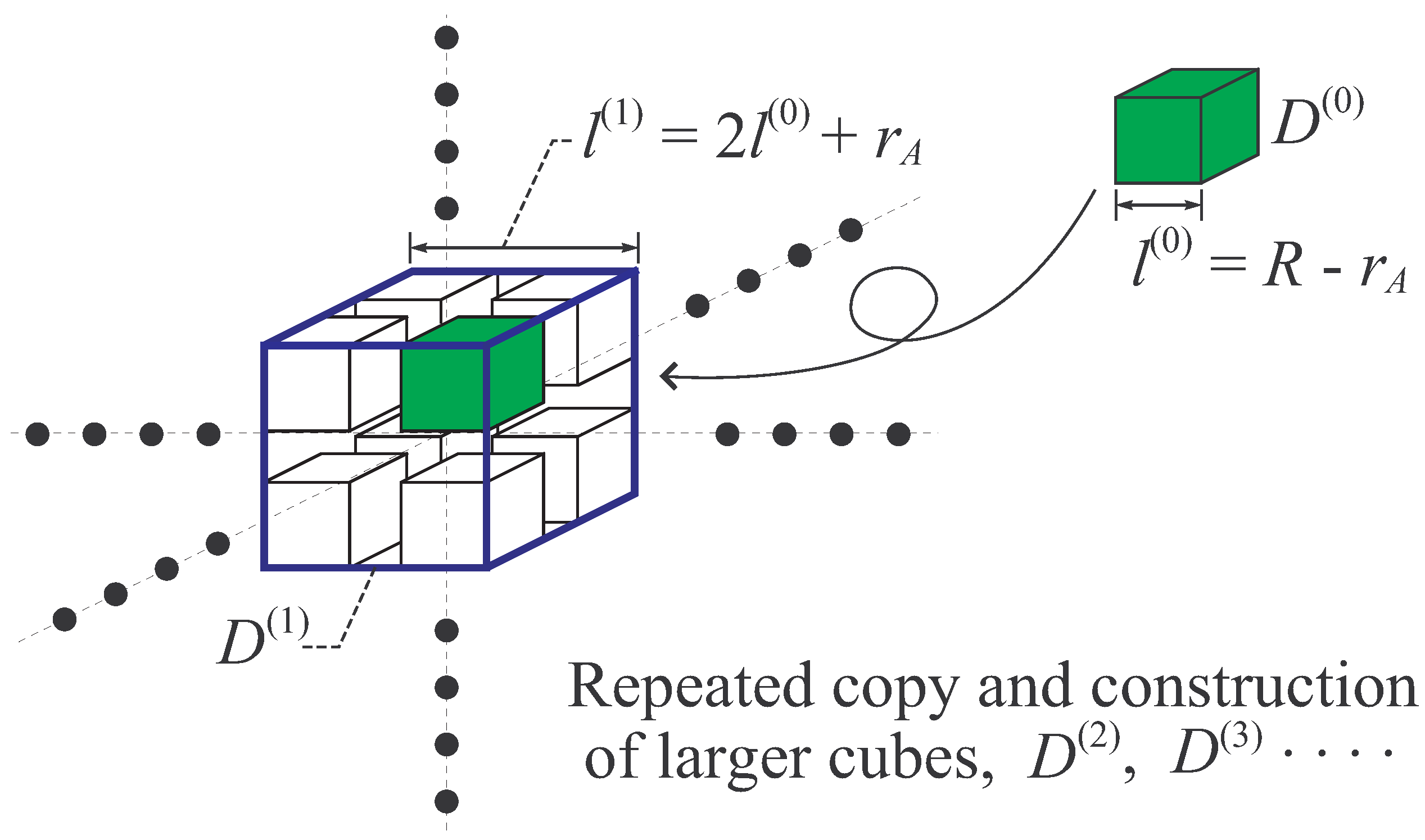
- Let be a cubic region of edge length , and denote its volume, . Then, make eight copies of the cube (including particles), and place them inside as shown in Figure 7 so as to share the eight vertices of with the eight copies of . By this construction of larger cube , the distance between smaller cubes is longer than or equal to . In the larger cube , there exist particles. The Hamiltonian of this system, , is expressed as that in Equation (70),where is defined as that in Equation (71). By the Condition A, holds.
- (iii)
- Let be a cubic region of edge length , and denote its volume. Repeat the procedure (ii) and construct the larger system in including particles with Hamiltonian, , where . Then, repeating again the same procedure n times, the n-th cube of edge length is constructed, which includes particles with Hamiltonian, , where . For sufficiently large n, we obtain a large system. Obviously, the Inequalities (77) and (79) can be applied to this large system with appropriate modifications.
B.4. Step 3 of the Proof: Result 2
B.4.1. Substep 3-1
B.4.2. Substep 3-2
B.4.3. Substep 3-3
C. Proof of Proposition 2
D. Preparations for Proposition 2
E. Proof of Corollary 1

© 2011 by the author; licensee MDPI, Basel, Switzerland. This article is an open access article distributed under the terms and conditions of the Creative Commons Attribution license (http://creativecommons.org/licenses/by/3.0/).
Share and Cite
Saida, H. Universal Property of Quantum Gravity implied by Uniqueness Theorem of Bekenstein-Hawking Entropy. Entropy 2011, 13, 1611-1647. https://doi.org/10.3390/e13091611
Saida H. Universal Property of Quantum Gravity implied by Uniqueness Theorem of Bekenstein-Hawking Entropy. Entropy. 2011; 13(9):1611-1647. https://doi.org/10.3390/e13091611
Chicago/Turabian StyleSaida, Hiromi. 2011. "Universal Property of Quantum Gravity implied by Uniqueness Theorem of Bekenstein-Hawking Entropy" Entropy 13, no. 9: 1611-1647. https://doi.org/10.3390/e13091611