Blind Deconvolution of Seismic Data Using f-Divergences

Abstract

This paper proposes a new approach to the seismic blind deconvolution problem in the case of band-limited seismic data characterized by low dominant frequency and short data records, based on Csiszár’s f-divergence. In order to model the probability density function of the deconvolved data, and obtain the closed form formula of Csiszár’s f-divergence, mixture Jones’ family of distributions (MJ) is introduced, by which a new criterion for blind deconvolution is constructed. By applying Neidell’s wavelet model to the inverse filter, we then make the optimization program for multivariate reduce to univariate case. Examples are provided showing the good performance of the method, even in low SNR situations.

1. Introduction

In seismic exploration, a seismic signal (e.g., recorded trace) is often represented as the result of a superposition of wavelets of constant shape weighted by the reflectivity series, thus it can be modeled as a convolution between the source signature (the embedded wavelet) and the reflectivity series. Deconvolution is an important process by which the reflectivity series can be estimated from the recorded trace, and vertical resolution of the seismic image will be enhanced.

For the above convolution model, when the wavelet is known, estimation of the reflectivity series is called deterministic deconvolution, which is done by least-squares, or in a Bayesian framework adding some priors on the reflectivity distribution.

As the wavelet is unknown, we have the classical blind deconvolution problem; statistical deconvolution appears to be a powerful tool for dealing with practical situations. Various approaches to statistical deconvolution have been proposed and applied in recent decades, including the expectation maximization (EM) algorithm, the higher-order statistics (HOS) algorithm, and the general purpose information criteria algorithm (GPIC).

The EM algorithm is an effective method for maximum-likelihood estimates, which are mainly used to estimate parameters from incomplete data. Since Mendel introduced the Bernoulli–Gaussian (BG) model as the distribution of reflectivity [1], a few approaches, based on the EM algorithm and BG model, have been published [2,3]. BG is a simple form of the Gaussian Mixture Model, which makes the likelihood function be expressible in closed form. The EM algorithm has shown good performance in the blind deconvolution context; whereby the estimation problem for the wavelet and reflectivity can be solved in an incomplete data set (the lack of localization and magnitude of the reflectivity). For the real field data, the reflectivity sequence changes do not always appear as clearly as predicted by the BG model [4], therefore, the sparse nature of the input signal is not a sufficiently robust hypothesis for good system estimation. On the other hand, it may be possible to extend the BG model to a more complicated probability density, however, the resulting expressions of the likelihood function will be handled inconveniently, adding obstacles for its use.

The higher-order statistics which we use are known as cumulants. The cumulant matching (CM) method has been developed for estimating a mix-phase wavelet from a convolutional process. Matching between the trace cumulant and the wavelet moment is done in a minimum mean-squared error sense under the assumption of a non-Gaussian, stationary and statistically independent reflectivity sequence. The main difficulty of this approach is that it requires a large amount of data to achieve reliable estimations [5]. But, in general, seismic data is arguably always nonstationary since anelastic attenuation processes are present everywhere, a seismic signal is shown to be approximately stationary just within a time window, in which the real signal is finite in length, leading to limited performance with this approach.

The GPIC algorithm has been intensively studied by many researchers for a large number of applications over the last couple of decades. In the seismic application, a seismic trace $x\left(n\right)$ may be written in the form:

$$x\left(n\right)=w\left(n\right)\ast r\left(n\right)+n\left(n\right)=s\left(n\right)+n\left(n\right)$$

(1)

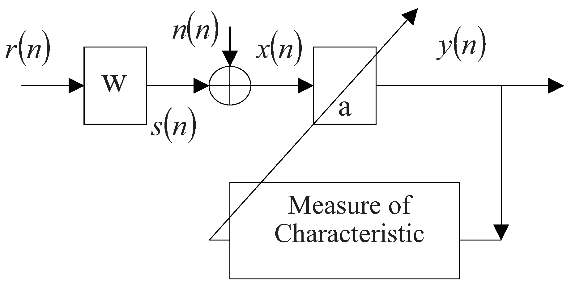
where $\ast$ denotes the convolution, $w\left(n\right)$, $r\left(n\right)$, $n\left(n\right)$ represent the wavelet, reflectivity, and superposed noise respectively. The idea of general purpose information criteria algorithm is to find an inverse filter $a$ to create an output:

$$y\left(n\right)=x\left(n\right)\ast a\left(n\right)$$

(2)

which looks like the reflectivity series, the inverse filter can be obtained by optimizing some criterion related to the output characteristic. Figure 1 depicts such a convolution-deconvolution system.

Figure 1. Convolution-deconvolution system.

Figure 1. Convolution-deconvolution system.

The earliest technique for this kind of algorithm was introduced by E.A. Robinson [6], and is based on the assumptions that the reflectivity sequence is a Gaussian white noise, and the wavelet is minimum phase. Since the pioneering work of Agard and Grau [7], it has been generally recognized in exploration geophysics that the reflectivity typically has a non-Gaussian distribution. Many techniques have been developed to exploit the nonGaussianity of seismic data for blind deconvolution based on information theory, among which excellent contributions were made by Wiggins, Claerbout, Gray, Ooe and Ulrych, Godfrey, Donoho, and Levy and Oldenburg [8,9,10,11,12,13,14], etc. For a more detailed discussion of their studies, see Walden [15].

Larue, Mars, and Jutten proposed a new blind single-input single-output (SISO) deconvolution method based on the minimization of the mutual information rate of the deconvolved output [4]. The mutual information has the nice property of being positive and it vanishes if and only if the components of deconvolved output are mutually independent, by which a good criterion for blind deconvolution can be obtained. They estimate deconvolution filter in the frequency domain. To take the band limited nature of seismic wavelets and the presence of noise into account, Baan and Pham presented a modification of the mutual-information rate, whitening the deconvolution output only within the wavelet pass band [16]. Their approach estimates the wavelet by maximizing the negentropy of the deconvolved output, and to prevent noise amplification, Wiener filtering is invoked.

Generally speaking, if a wavelet has no zeros on the unit circle, blind deconvolution is a well posed problem, but if it has zeros on the unit circle, then the problem is ill posed, in which the only criterion to apply to inverse filter is to maximize the nonGaussianity of the deconvolved output according to the central limit theorem, provided the distribution of reflectivity is non-Gaussian and non-infinite divisibility. In Van der Baan and Pham’s work, they use negentropy as a criterion to perform deconvolution, which is defined as the Kullback-Liebler divergence between the density and the normal equivalent i.e. with the same mean and variance.

In statistics and information theory, Kullback-Liebler divergence is just one of information measures to show the difference of two distributions, Csiszár (and independently also by Ali and Silvery) introduced the f-divergence yielding a generalized family of invariant measures, which is given by [17]:

$$D_f\left(p,q\right)={\displaystyle \int q\left(x\right)f\left(\frac{p\left(x\right)}{q\left(x\right)}\right)}dx$$

(3)

for convex $f:\left(0,\infty \right)\to R$, and $f\left(1\right)=0$, where $p$ and $q$ are two probability density functions (PDF). For $f\left(x\right)=x\ln x$, the f-divergence reduces to the classical Kullback-Liebler divergence.

Considering a real value convex function $g$ defined on $R$, from classical Jensen inequality:

$$Eg\left(X\right)\ge g\left(EX\right)$$

(4)

we have:

$$D_f\left(p,q\right)\ge f\left({\displaystyle \int q\left(x\right)\frac{p\left(x\right)}{q\left(x\right)}}dx\right)=f\left(1\right)=0$$

(5)

Equality holds if and only if $p=q$. If we use $p$ to denote the PDF of the deconvolution output, and let $q$ be a PDF of the normal distribution with the same variance as that of $p$, then f-divergence is nonnegative and scale invariant, and will become larger as the deconvolution output goes off the Gaussianity, which provides an appealing method to build an information criterion.

In the above entropy-based approaches by Larue, Mars, and Jutten, Baan and Pham, one key point is to estimate the PDF of the deconvolution output, therefore, Pham designed a fast algorithm to obtain the PDF and score function for blind source separation application. However, as a nonparametric method, Pham’s fast algorithm needs certain length of the data to provide a good estimation, in their deconvolution examples, the length of the input data is usually over 500. As mentioned above, a seismic signal is treated to be stationary just within a limited time window due to the intrinsic attenuation of the earth medium, these entropy-based approaches seem to result in a limited performance in the case of short data records.

Another point for the above approaches is that the number of iterations depends strongly on the choice of initialization of inverse filter, as most optimization programs do. Thirdly, to improve the stability and the performance of the algorithm, some constraints need to be placed on the inverse filter when deconvolution criterion are to be proposed, which can bring in some artifacts.

Inspired by Larue, Mars, and Jutten, Baan and Pham’s works, this paper aims at constructing new criterion based on Csiszár f-divergence for seismic deconvolution, and proposes a new blind deconvolution algorithm. This new method can handle data with small samples, which means it has ability to deal with nonstationary data. We believe this approach is novel for several reasons:

• To facilitate estimating the PDF of the deconvolution output, we use mixture Jones’ family of distributions (MJ) to model the PDF of the output, by this way; the PDF to be estimated can be generated with only several parameters;
• We derive the closed form formula for one kind of Csiszár f-divergence by applying MJ distribution, from which a new criterion for blind deconvolution can be constructed;
• We apply the wavelet model derived by Neidell to design the inverse filter; this wavelet model has two shape parameters. If we know the dominant frequency of the wavelet, only one parameter is left, which means the optimization program for multivariate reduces to univariate case without setting initialization and adding constraint on inverse filter.

The rest of the paper is organized as follows. In Section 2 we briefly introduce the MJ distribution. Based on the MJ distribution, in Section 3, we derive one of the Csiszár f-divergences in closed form. In Section 4, we introduce the parameter estimation of this MJ distribution from the real data. After briefly introducing the wavelet model derived by Neidell in Section 5, we describe our deconvolution procedure in Section 6. Examples illustrating the effectiveness of our approach are given in Section 7. Finally, we give a briefly discussion on the wavelet phase estimation in Section 8. We give the conclusions in Section 9.

2. MJ Distribution

Jones constructed a family of distributions arising from distributions of order statistics, and it has a PDF to be of the form [18]:

$$f\left(x\right)=\frac{c\left(x\right)}{B\left(a,b\right)}{C}^{a-1}\left(x\right){\left(1-C\left(x\right)\right)}^{b-1},a>0,b>0$$

(6)

where $B$ is the complete beta function, $c$ is a PDF simply symmetric about zero, its distribution function is $C$, i.e., $C^{\prime }=c$.

The Roles of a and b are that:

• For $a=b=1$, $f=c$;
• If $a=b$, the corresponding distributions remain symmetric;
• If $a\ne b$, skewness is introduced;
• $a$ controls left-hand tail weight, $b$ controls right; the smaller $a$ or $b,$ the heavier the corresponding tail.

Figure 2 shows some examples of symmetric Jones’ family of distributions generated from the standard normal distribution.

Figure 2. Examples of symmetric Jones’ family of distributions.

Figure 2. Examples of symmetric Jones’ family of distributions.

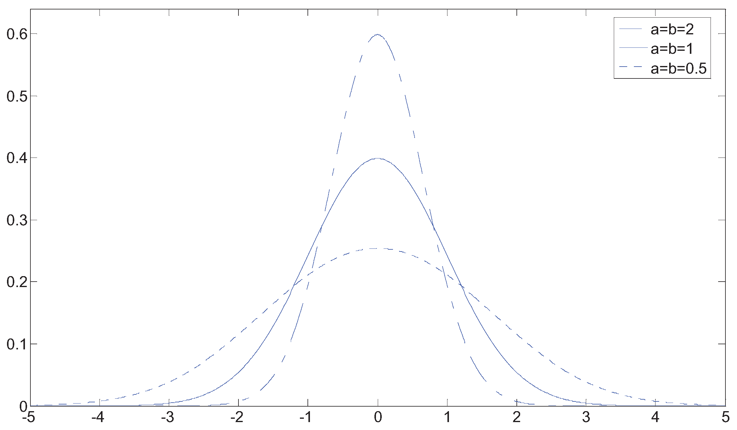
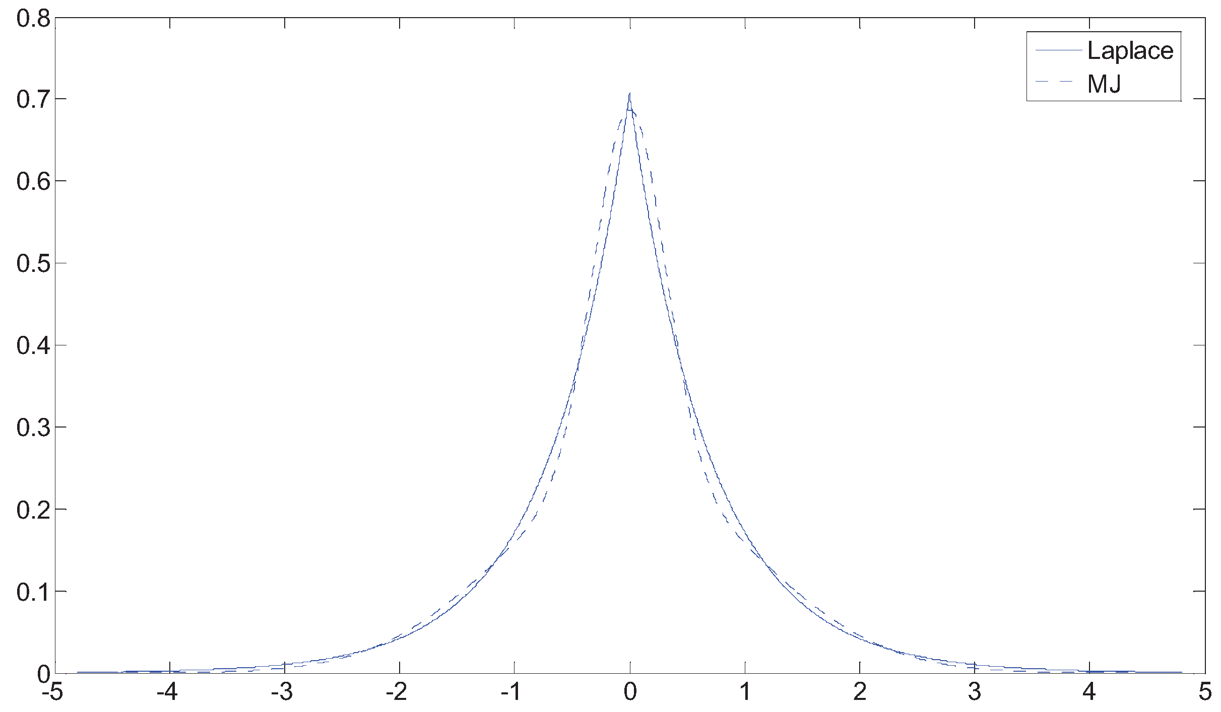
From Figure 2, we can see that a large family of distributions can be generated with this family; unfortunately a single Jones’ family of distributions can only depict the tailedness or peakedness of a PDF, in practice, the distribution of reflectivity is essentially symmetric, with a sharper central peak and larger tails than a Gaussian distribution. In order to fit both tailedness and peakedness of the real data, we introduce the mixture Jones’ family of distributions (MJ), which has the form:

$$f\left(x\right)=\left(\lambda \frac{G^{{\alpha }_1-1}\left(x\right){\left(1-G\left(x\right)\right)}^{{\alpha }_1-1}}{B\left({\alpha }_1,{\alpha }_1\right)}+\left(1-\lambda \right)\frac{G^{{\alpha }_2-1}\left(x\right){\left(1-G\left(x\right)\right)}^{{\alpha }_2-1}}{B\left({\alpha }_2,{\alpha }_2\right)}\right)g\left(x\right)$$

(7)

where $\lambda \in \left[0,1\right]$, $0<{\alpha }_1<1$, which controls the tail of $f$. ${\alpha }_2\ge 1$, which controls the peak of $f$. $g$ is the PDF of a normal distribution random variable with zero mean and the same variance as that of real data, $G$ is the distribution function of $g$, $G^{\prime }=g$.

Figure 3 shows an example of fitting a Laplace distribution with unit standard deviation using MJ, where $g$ takes the form of the standard normal distribution.

Figure 3. Fitted Laplace distribution Using MJ.

Figure 3. Fitted Laplace distribution Using MJ.

3. Measures of Non-gaussianity Using f-Divergence

The goal of introducing an MJ distribution is to obtain the closed form formulas for the Csiszár f-divergence. In the equality (3), if we take one of the distributions as normal distribution with zero mean and the same variance as that of real data, then the f-divergence can indicate the non-Gaussianity of the data. Among the different Csiszár f-divergences, the following measure is considered in this paper:

$$D\left(p,q\right)={\displaystyle \int \frac{{\left(p-q\right)}^2}{p}}dx$$

(8)

which is also called Kagan distance.

Let us compute the above divergence with respect to the MJ distribution; using (8), we have:

$$\begin{array}{cc}D\left(f,g\right)& ={\displaystyle {\int }_{-\infty }^{\infty }\frac{{\left(f-g\right)}^2}{g}}dx={{\displaystyle {\int }_{-\infty }^{\infty }\left(\frac{f}{g}-1\right)}}^{2}gdx\hfill \\ & ={{\displaystyle {\int }_{-\infty }^{\infty }\left(\lambda \frac{G^{{\alpha }_1-1}{\left(1-G\right)}^{{\alpha }_1-1}}{B\left({\alpha }_1,{\alpha }_1\right)}+\left(1-\lambda \right)\frac{G^{{\alpha }_2-1}{\left(1-G\right)}^{{\alpha }_2-1}}{B\left({\alpha }_2,{\alpha }_2\right)}-1\right)}}^{2}gdx\hfill \end{array}$$

(9)

Noting that $\frac{dG}{dx}=g$, and $G$ is a distribution function, the change of variable $y=G\left(x\right)$, $dy=gdx$ yields:

$$\begin{array}{cc}D\left(f,g\right)& ={{\displaystyle {\int }_0^1\left(\lambda \frac{y^{{\alpha }_1-1}{\left(1-y\right)}^{{\alpha }_1-1}}{B\left({\alpha }_1,{\alpha }_2\right)}+\left(1-\lambda \right)\frac{y^{{\alpha }_2-1}{\left(1-y\right)}^{{\alpha }_2-1}}{B\left({\alpha }_2,{\alpha }_2\right)}-1\right)}}^{2}dy\hfill \\ & ={\lambda }^2\frac{B\left(2{\alpha }_1-1,2{\alpha }_1-1\right)}{B^2\left({\alpha }_1,{\alpha }_1\right)}+{\left(1-\lambda \right)}^2\frac{B\left(2{\alpha }_2-1,2{\alpha }_2-1\right)}{B^2\left({\alpha }_2,{\alpha }_2\right)}\hfill \\ & +2\lambda \left(1-\lambda \right)\frac{B\left({\alpha }_1+{\alpha }_2-1,{\alpha }_1+{\alpha }_2-1\right)}{B\left({\alpha }_1,{\alpha }_1\right)B\left({\alpha }_2,{\alpha }_2\right)}-1\hfill \end{array}$$

(10)

4. Estimation of the Parameters of the MJ Distribution

From the equality (7), let $y=G\left(x\right)$, the resulting distribution is a mixture Beta distribution, which takes the form:

$$h\left(y\right)=\lambda \frac{y^{{\alpha }_1-1}{\left(1-y\right)}^{{\alpha }_1-1}}{B\left({\alpha }_1,{\alpha }_1\right)}+\left(1-\lambda \right)\frac{y^{{\alpha }_2-1}{\left(1-y\right)}^{{\alpha }_2-1}}{B\left({\alpha }_2,{\alpha }_2\right)}\begin{array}{cc}& y\in \left[0,1\right]\end{array}$$

(11)

then the parameters can be estimated by resorting to the method of moments.

We use the expectation of function $y^{n-1}{\left(1-y\right)}^{n-1}$ with respect to this mixture Beta distribution to perform the parameter estimation, which can be written as:

$$\begin{array}{cc}M\left(n\right)\hfill & ={\displaystyle {\int }_0^1{y}^{n-1}}{\left(1-y\right)}^{n-1}h\left(y\right)dy\hfill \\ & =\lambda \frac{B\left({\alpha }_1+n-1,{\alpha }_1+n-1\right)}{B\left({\alpha }_1,{\alpha }_1\right)}+\left(1-\lambda \right)\frac{B\left({\alpha }_2+n-1,{\alpha }_2+n-1\right)}{B\left({\alpha }_2,{\alpha }_2\right)}\hfill \end{array}$$

(12)

Noting that $B\left(\alpha ,\beta \right)=\Gamma \left(\alpha \right)\Gamma \left(\beta \right)/\Gamma \left(\alpha +\beta \right)$, and $\Gamma \left(\alpha +1\right)=\alpha \Gamma \left(\alpha \right)$, we can expand the expression (12) as:

$$M\left(n\right)=\lambda \frac{{\displaystyle \prod _{k=0}^{n-2}{\left({\alpha }_1+k\right)}^2}}{{\displaystyle \prod _{k=0}^{2n-3}\left(2{\alpha }_1+k\right)}}+\left(1-\lambda \right)\frac{{\displaystyle \prod _{k=0}^{n-2}{\left({\alpha }_2+k\right)}^2}}{{\displaystyle \prod _{k=0}^{2n-3}\left(2{\alpha }_2+k\right)}}\begin{array}{cc}& n\ge 2\end{array}$$

(13)

By choosing $n=2,3,4$ in (13) respectively, and simplifying, we have:

$$\frac{\lambda }{2{\alpha }_1+1}+\frac{1-\lambda }{2{\alpha }_2+1}={\theta }_1$$

(14)

$$\frac{\lambda }{2{\alpha }_1+3}+\frac{1-\lambda }{2{\alpha }_2+3}={\theta }_2$$

(15)

$$\frac{\lambda }{2{\alpha }_1+5}+\frac{1-\lambda }{2{\alpha }_2+5}={\theta }_3$$

(16)

where:

$${\theta }_1=1-4M\left(2\right)$$

(17)

$${\theta }_2=\frac{1}{3}\left(2-{\theta }_1-32M\left(3\right)\right)$$

(18)

$${\theta }_3=\frac{4}{15}\left(2-\frac{3}{4}{\theta }_1-7{\theta }_2-128M\left(4\right)\right)$$

(19)

Replacing $2{\alpha }_1+3$ and $2{\alpha }_2+3$ in (15) by $x_1$ and $x_2$, from (14), (15), (16) we have:

$$\frac{\lambda }{x_1-2}+\frac{1-\lambda }{x_2-2}={\theta }_1$$

(20)

$$\frac{\lambda }{x_1}+\frac{1-\lambda }{x_2}={\theta }_2$$

(21)

$$\frac{\lambda }{x_1+2}+\frac{1-\lambda }{x_2+2}={\theta }_3$$

(22)

After some simple algebraic calculations, we obtain:

$$\left({\theta }_2-{\theta }_1\right)x_1{x}_2+2{\theta }_1\left(x_1+x_2\right)=4{\theta }_1+2$$

(23)

$$\left({\theta }_2-{\theta }_3\right)x_1{x}_2-2{\theta }_3\left(x_1+x_2\right)=4{\theta }_3-2$$

(24)

Then, we have:

$$\left[\begin{array}{c}{x}_1{x}_2\\ x_1+x_2\end{array}\right]={\left[\begin{array}{cc}{\theta }_2-{\theta }_1& 2{\theta }_1\\ {\theta }_2-{\theta }_3& -2{\theta }_3\end{array}\right]}^{-1}\left[\begin{array}{c}4{\theta }_1+2\\ 4{\theta }_3-2\end{array}\right]=\left[\begin{array}{c}{\xi }_1\\ {\xi }_2\end{array}\right]$$

(25)

So, $x_1$ and $x_2$ are the solutions of equation:

$$x^2-{\xi }_{2}x+{\xi }_1=0$$

(26)

Hence, we can show that the corresponding parameters is estimated as:

$${\widehat{\alpha }}_1=\frac{\min \left(x_1,x_2\right)-3}{2}$$

(27)

$${\widehat{\alpha }}_2=\frac{\max \left(x_1,x_2\right)-3}{2}$$

(28)

$$\widehat{\lambda }=\frac{{\theta }_2{\xi }_1-\min \left(x_1,x_2\right)}{\sqrt{{\xi }_2^2-4{\xi }_1}}$$

(29)

Based on above results, we have the estimation of the JM parameters as follows:

• Estimate the variance ${\sigma }_y^2$ of the output $\left\{y_n\right\}$ of the inverse filter;
• Transform the data $\left\{y_n\right\}$ into.

  $$z_n=G\left(y_n\right)=\frac{1}{{\sigma }_y\sqrt{2\pi }}{\displaystyle {\int }_{-\infty }^{y_n}{e}^{-\frac{t^2}{2{\sigma }_y^2}}}dt$$

  (30)
• Estimate the $M\left(2\right)$, $M\left(3\right)$ and $M\left(4\right)$ of $\left\{z_n\right\}$;
• Compute parameters of MJ using corresponding equalities.

5. On the Inverse Filter

Following the work by Baan and Pham, we can show that if the wavelet is known, the Wiener filter achieves an optimum solution for the inverse filter, since it makes a compromise between signal recovery and noise reduction. In the frequency domain, it can be written as:

$$A_{opt}\left(\omega \right)=\frac{\overline{W}\left(\omega \right)}{{\left|W\left(\omega \right)\right|}^2+{\epsilon }^2}$$

(31)

where $W\left(\omega \right)$ is the wavelet, the superscript of the numerator denotes the complex conjugate, ${\epsilon }^2$ is a normalization factor.

In the blind deconvolution context, the wavelet is unknown, and needs to be estimated, therefore, we adopt Neidell’s wavelet model to construct an inverse filter, which is derived from practical observation, and its z transform has the form [19]:

$$W_N\left(Z\right)={\left(1-Z\right)}^n{\left(1+Z\right)}^m\begin{array}{cc}& n>0,m>0\end{array}$$

(32)

furthermore, if we denote the peak frequency of the amplitude spectrum of this wavelet as ${\omega }_p$, the relationship between the $n$ and $m$ is:

$$\cos {\omega }_p=\frac{m-n}{m+n}$$

(33)

So, if we know the peak frequency of the amplitude spectrum of the real wavelet, only one parameter needs to be determined, in practice, usually we do not know it; we have following value as a substitution for ${\omega }_p$:

$${\widehat{\omega }}_p=\underset{\omega }{\arg }\max \left|FT\left(x_n\right)\right|$$

(34)

where $FT$ denotes Fourier transform, $\left\{x_n\right\}$ denotes the seismic record.

6. New Deconvolution Algorithm

Based on the above results, we construct a new frequency-domain criterion for blind deconvolution:

$$J\left(A\right)=D\left(f,g\right)$$

(35)

After determining the ${\omega }_p$, $J\left(A\right)$ is just the function of $n$ or $m$, so we have:

$$n_{opt}=\underset{n}{\arg }\max J$$

(36)

$$A_{opt}\left(\omega \right)=\frac{{\overline{W}}_N\left(n_{opt},\omega \right)}{{\left|W_N\left(n_{opt},\omega \right)\right|}^2+{\epsilon }^2}$$

(37)

Thus our new deconvolution algorithm consists of the following steps:

• Estimate ${\omega }_p$ of the real data $\left\{x_n\right\}$;
• Compute the output $\left\{y_n^n\right\}$ of the inverse filter with the different parameter $n$, in which the superscript $n$ denotes the shape parameter of the inverse filter; the subscript denotes the number of the time series $y$, and the inverse filter is given by (31) and (32);
• Estimate the MJ parameters $\left\{{\widehat{\alpha }}_1^n,{\widehat{\alpha }}_2^n,{\widehat{\lambda }}_n\right\}$ of the corresponding output of the inverse filter using the method in section four, and compute the information distance $D_n\left(f_n,g_n\right)$;
• Search the maximum cost function $J\left(A\right)$ to get the optimum inverse filter.

7. Results

In this section, we evaluate the performance of the proposed method through simulations and real experimental data.

7.1. Simulation Results

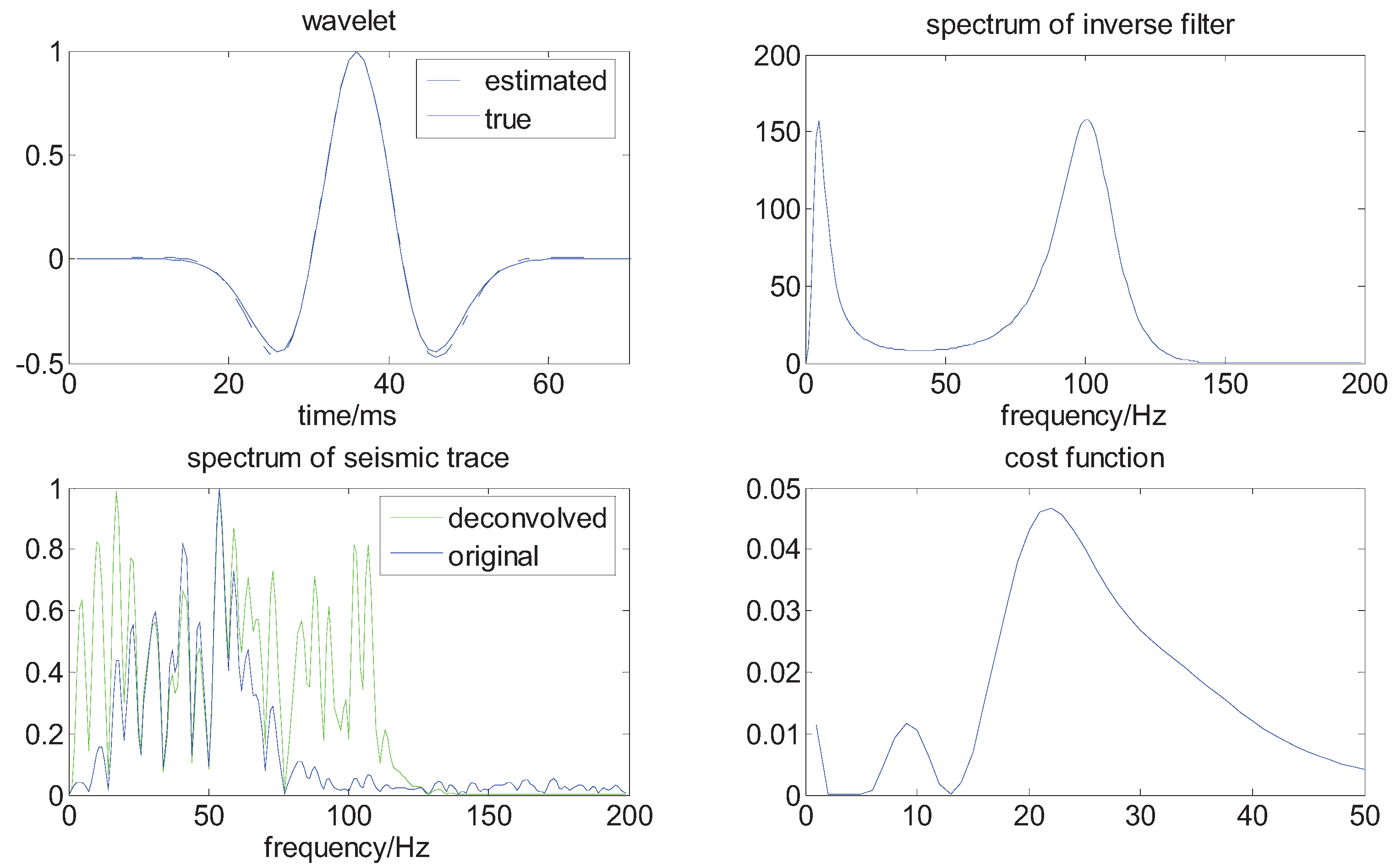
We build a synthetic trace by convolving a super-Gaussian reflectivity with a Ricker wavelet; the wavelet has zero phase and a central frequency of 40 Hz. The reflectivity is generated as $b^3\left(n\right)$, where $b\left(n\right)$ are independent normal random variables with zero mean and variance 0.28, the sample interval is 1 ms. In order to test the performance of our methods for the data with small samples, we set the length of the synthetic trace about 256. The results are plotted in Figure 4 and Figure 5.

Figure 4. The results of deconvolution in the noise-free case.

Figure 4. The results of deconvolution in the noise-free case.

Figure 5. The contrast between the original trace and the deconvolved trace.

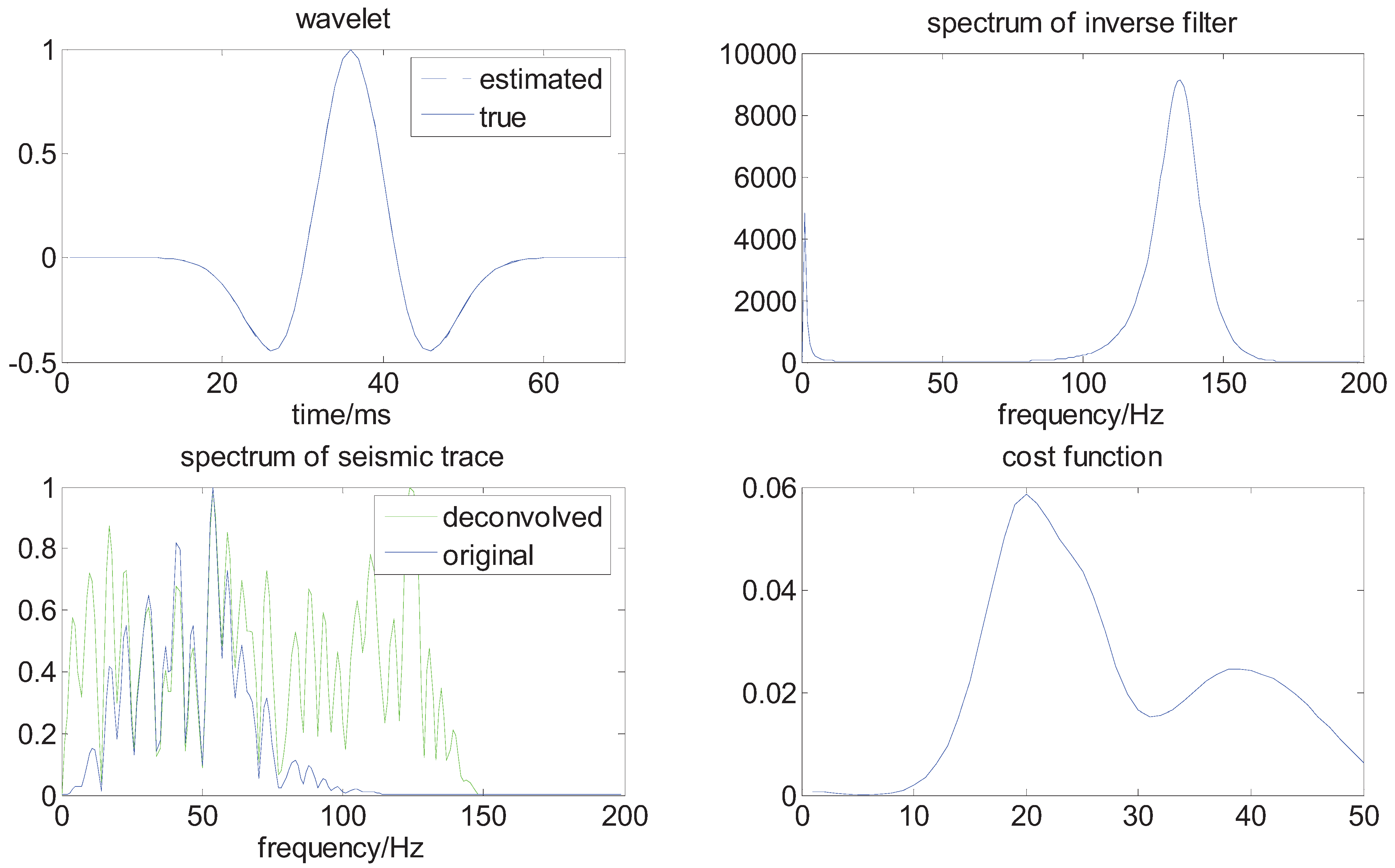
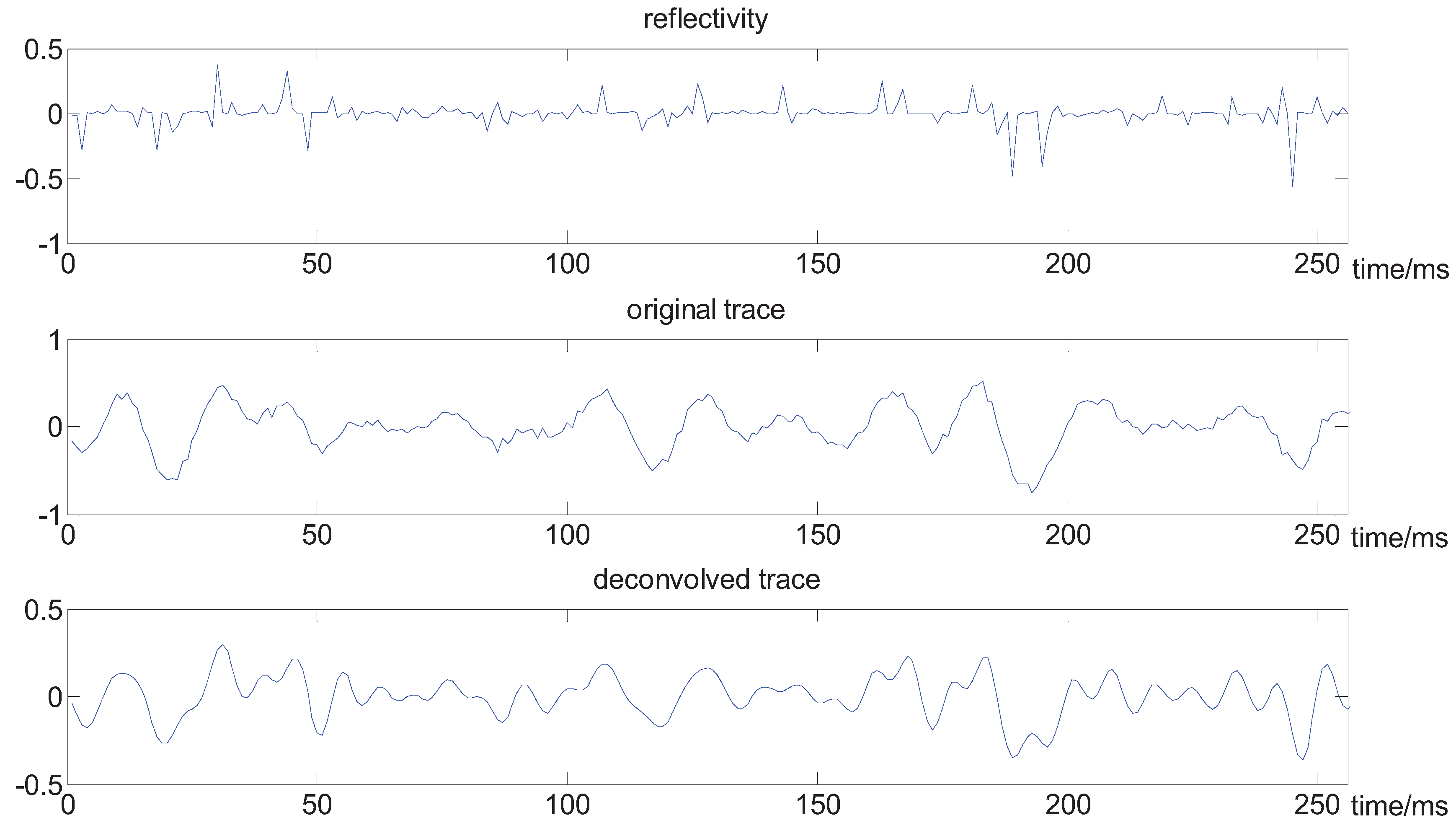
Figure 5. The contrast between the original trace and the deconvolved trace.

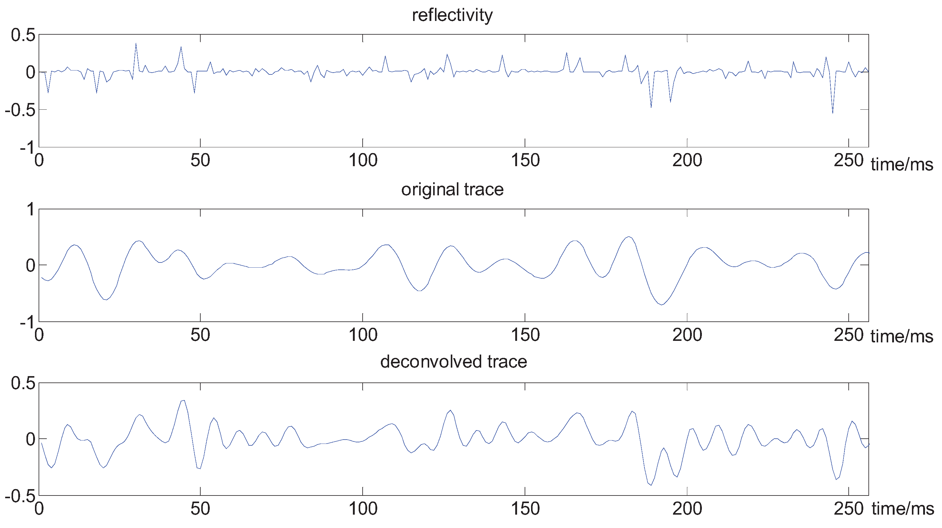
From the above figures, we can see that the wavelet is well estimated, and the spectrum of the seismic trace is obviously broadened, the deconvolved seismic data has an improved vertical resolution; for example, there are two big seismic reflectors near 200 ms, which cannot be separated in the original seismic trace; in the deconvolved trace, they are well distinguished, and some layer interfaces are thinner and better localized.

In the previous experiment, we used noiseless signals. Since the blind deconvolution methods are very sensitive to additive noise, it is important to test our algorithm for noisy signals. To this end, we add some noise to the synthetic trace, where the resulting signal-to-noise ratio is 15 dB. The results are plotted in Figure 6 and Figure 7, in which it can be shown that our method provides a good trade-off between deconvolution and noise amplification.

Figure 6. The results of deconvolution for a noisy signal.

Figure 6. The results of deconvolution for a noisy signal.

Figure 7. The contrast in the case of noise.

Figure 7. The contrast in the case of noise.

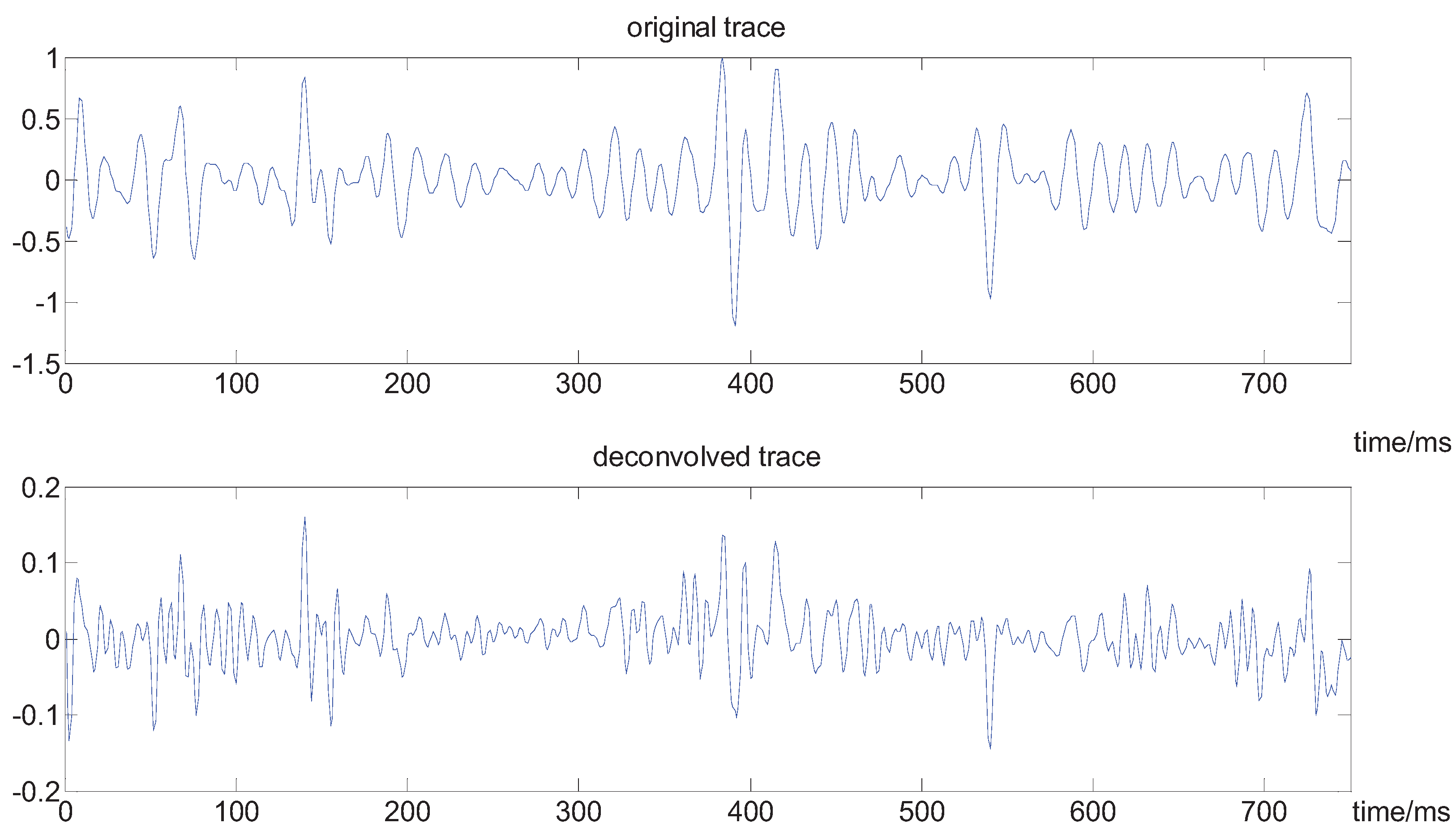
7.2. Real-Data Experiment

Here we adopt our method to a real seismic dataseat, which is from the CHANGQING oil field in China. The original data contains about 750 samples. From Figure 8 and Figure 9, we can see the spectrum of the seismic trace is broadened, and the resolution of seismic record is improved. For instance, the seismic reflectors, localized in about the 170 point, 400 point and the end of the trace, respectively, are now well imaged.

Figure 8. The contrast in the spectrum of the seismic trace.

Figure 8. The contrast in the spectrum of the seismic trace.

Figure 9. The contrast in the waveform of the seismic trace.

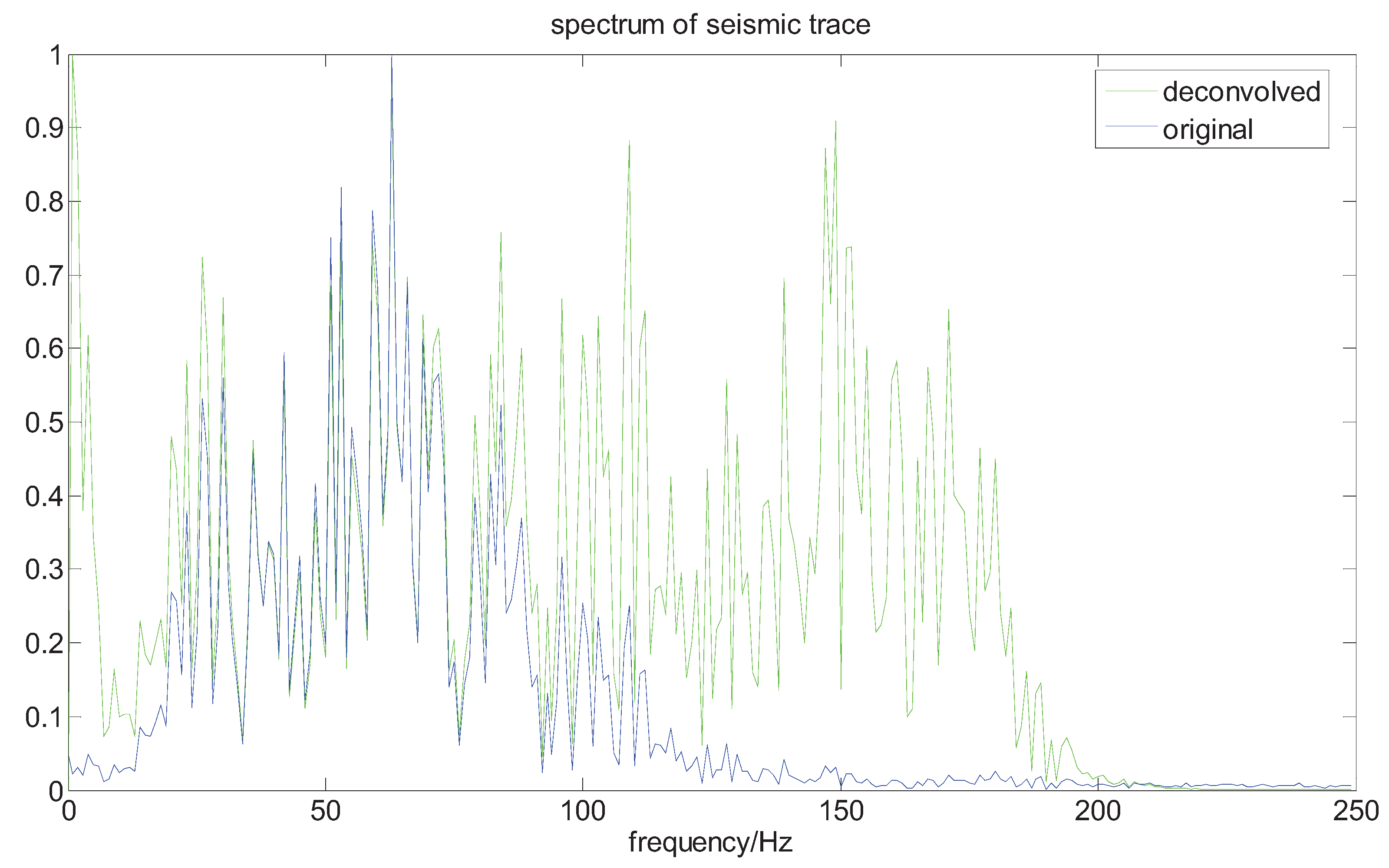
Figure 9. The contrast in the waveform of the seismic trace.

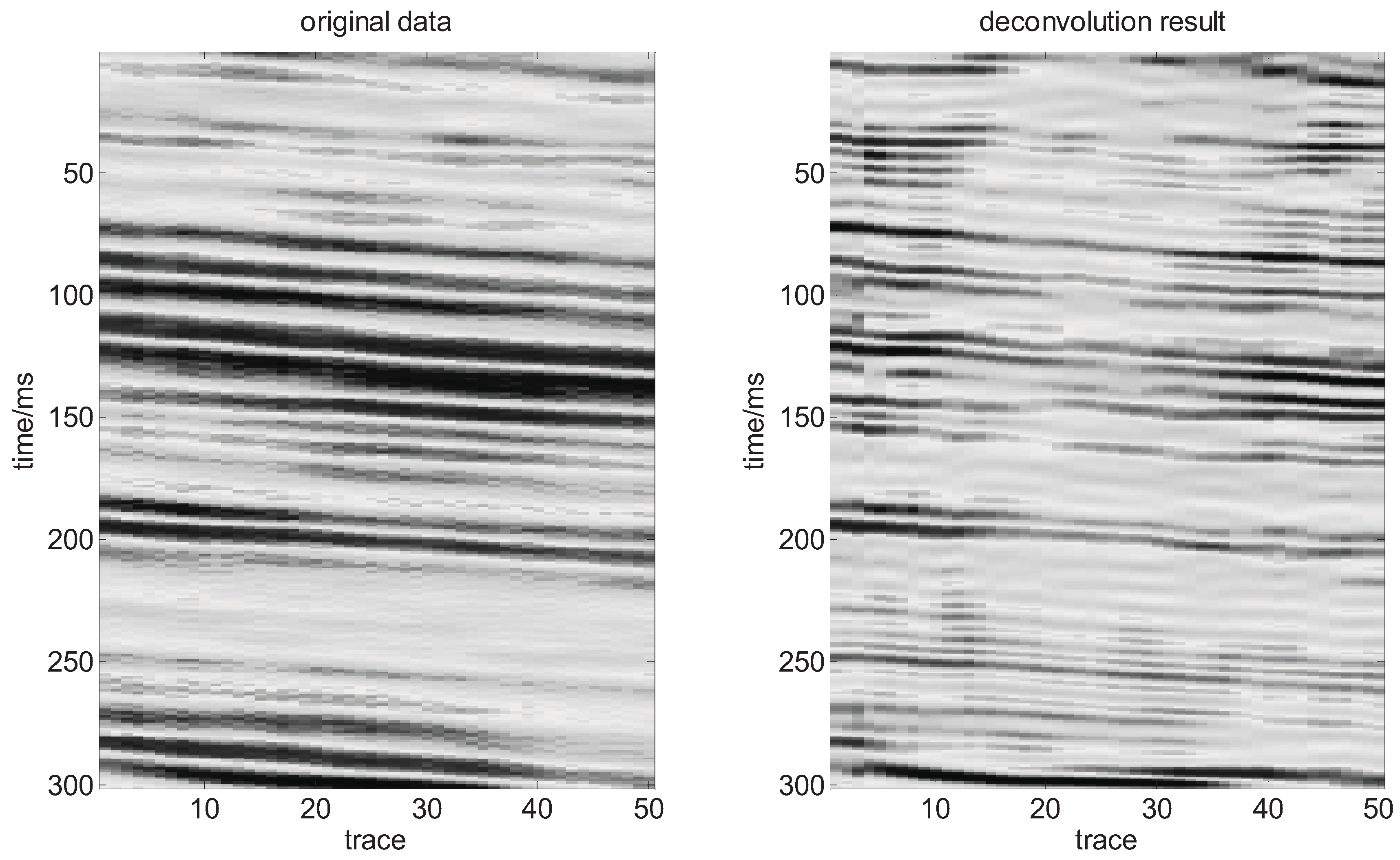
7.3. Stacked Section

In the final example, a stacked section is considered which is from CNOOC Research Center. Figures 10 display the data before and after deconvolution by our method. Comparing the seismic data before and after deconvolution, we can see that the deconvolved seismic data shows a significant improvement in vertical resolution and enhanced reflection detail corresponding to the geology. Such high-resolution reflection detail is a desirable feature for seismic interpretation. This example indicates that the method can work well in practice and can properly enhance the resolution of the seismic data.

Figure 10. Deconvolution result for stacked section.

Figure 10. Deconvolution result for stacked section.

8. Discussion

In our simulation experiments, the wavelet is zero phase, which means that our method performs well for zero-phase deconvolution. Zero-phase deconvolution, also denoted as pure-amplitude deonvolution, leaves the phase of original seismic section undistorted after deconvolution, i.e. with no time shift. However, in the blind deconvolution context, it is important for an algorithm to estimate well the phase of the wavelet. Theoretically, if a wavelet is reversible, i.e., no zeros on the unit circle, its phase can be uniquely determined (or a linear phase shift is left) by the non-Gaussianity maximization of the deconvolved output, As far as the irreversible wavelet, i.e., band-limited wavelet, is concerned, to our knowledge, there are no sound theoretical reasons for determining the phase of the wavelet uniquely.

To test the performance of these information-based approaches for the band-limited wavelet phase estimation, we designed the following experiment. Firstly we use a band-pass filter with constant phase to approximately model the spectrum of the deconvolved wavelet, which takes the form:

$$C_k\left(\omega \right)=\{\begin{array}{cc}{e}^{\pm j\frac{k\pi }{N-1}}& k=0,1,\cdots ,N-1,{\omega }_L\le \left|\omega \right|\le {\omega }_H\\ 0& else\end{array}$$

(38)

where if the frequency of the band-pass filter is positive, the plus sign is taken.

Secondly, we apply this band-pass filter bank to a reflectivity, and get a series of outputs; it is immediate that the information distance $D\left(f,g\right)$ is the function of $k$. After having computed the information distances corresponding to different $k$, we can find the unique $k_m$, for which the information distance achieves its peak value. If $k_m=0$ or $N-1$, it shows that the algorithm based on the non-Gaussianity maximization can make a good estimation for the phase of the band-limited wavelet. Finally, we independently perform the above experiment many times to obtain a numerical result.

Considering the real situation, in which the dominant frequency of the wavelet is low, we choose a Ricker wavelet with a central frequency 40 Hz, hence, the high frequency of the band-pass filter is 120 Hz, in the meantime, we set the low frequency as 5 Hz, and $N=20$. The reflectivity contains 256 sampling points, and is generated as $b^3\left(n\right)$, where $b\left(n\right)$ are independent normal random variables with zero mean and variance 0.28. The result of 100 independent trials is plotted in Figure 11.

Figure 11. The histogram of $k_m$.

Figure 11. The histogram of $k_m$.

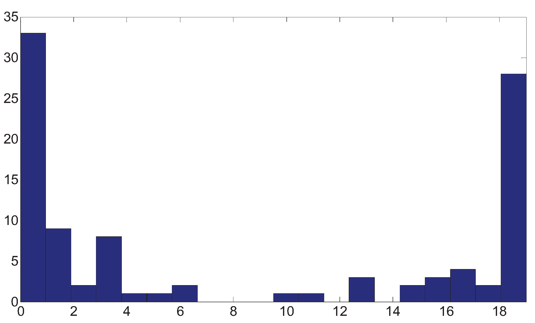
Form the histogram of $k_m$, it can be shown that about 60% of the $k_m$ take the value of $0$ or $N-1$, there is still some randomness in the phase estimation in the case of band-limited seismic data with a low dominant frequency and short data records.

9. Conclusions

In this paper, we have presented a new blind deconvolution method based on Csiszár f-divergence in the frequency domain. To facilitate estimating the PDF of the deconvolution output and deriving the closed form formulas of Csiszár f-divergence, we use MJ distribution to model the PDF of the output, and in this way, the PDF to be estimated can be generated with only a few parameters, and a new criterion for blind deconvolution can be constructed. Furthermore, we apply the wavelet model derived by Neidell to the inverse filter, which means the optimization program for multivariate reduces to univariate case without setting initialization and adding constraints to the inverse filter. The method has been applied to synthetic and real traces. Simulations and real-data experiments have shown the ability of our approach in the presence of the band-limited seismic data with a low dominant frequency, short data records, and low signal-to-noise ratio.

References

- Kormylo, J.; Mendel, J.M. Maximum Likelihood detection and estimation of Bernoulli-Gaussian porcesses. IEEE Trans. Inf. Theory 1982, 28, 482–488. [Google Scholar] [CrossRef]
- Rosec, O.; Boucher, J.M.; Nsiri, B.; Chonavel, T. Blind Marine seismic deconvolution using statistical MCMC methods. IEEE J. Ocean. Eng. 2003, 28, 502–512. [Google Scholar] [CrossRef]
- Nsiri, B.; Chonavel, T.; Boucher, J.-M.; Nouze, H. Blind submarine seismic deconvolution for long source wavelets. IEEE J. Ocean. Eng. 2007, 32, 729–743. [Google Scholar] [CrossRef]
- Larue, A.; Mars, J.I.; Jutten, C. Frequency-domain blind deconvolution based on mutual information rate. IEEE Trans. Signal Process. 2006, 54, 1771–1781. [Google Scholar] [CrossRef]
- Lazear, G.D. Mixed-phase wavelet estimation using fourth-order cumulants. Geophysics 1993, 58, 1042–1051. [Google Scholar] [CrossRef]
- Robinson, E.A. Predictive decomposition of time series with application to seismic exploration. Geophysics 1967, 32, 418–484. [Google Scholar] [CrossRef]
- Agard, J.; Grau, G. Etude statistique de sismogrammes. Geophys. Prospect. 1961, 9, 503–525. [Google Scholar] [CrossRef]
- Wiggins, R.A. Minimum entropy deconvolution. Geoexploration 1978, 16, 21–35. [Google Scholar] [CrossRef]
- Claerbourt, J.F. Parsimonious deconvolution. Stanf. Explor. Project 1977, 13, 1–9. [Google Scholar]
- Gray, W. Variable Norm Deconvolution. Ph.D. Thesis, Stanford University, Palo Alto, CA, USA, 1979. [Google Scholar]
- Ooe, M.; Ulrychm, T.J. Minimum entropy deconvolution with an exponential transformation. Geophys. Prosp. 1979, 27, 458–437. [Google Scholar] [CrossRef]
- Godfrey, R. An information theory approach to deconvolution. Stanf. Explor. Project 1978, 15, 157–182. [Google Scholar]
- Donoho, D. On Minimum Entropy Deconvolution; Academic Press Inc.: San Diego, CA, USA, 1981. [Google Scholar]
- Levy, S.; Oldenburg, D.W. Automatic phase correction of common-midpoint stacked data. Geophysics 1987, 52, 51–59. [Google Scholar] [CrossRef]
- Walden, A.T. Non-Gaussian reflectivity, entropy, and deconvolution. Geophysics 1985, 50, 2862–2888. [Google Scholar] [CrossRef]
- Baan, M.V.; Pham, D.T. Robust wavelet estimation and blind deconvolution of noisy surface seismics. Geophysics 2008, 73, V37–V46. [Google Scholar] [CrossRef]
- Csiszar, I. Information-type measures of difference of probability distributions and indirect. Stud. Sci. Math. Hung. 1967, 2, 299–318. [Google Scholar]
- Jones, M.C. Families of distributions arising from distributions of order statistics. Test 2004, 13, 1–43. [Google Scholar] [CrossRef]
- Neidell, N.S. Could the processed seismic wavelet be simpler than we think? Geophysics 1991, 56, 681–690. [Google Scholar] [CrossRef]
© 2011 by the authors; licensee MDPI, Basel, Switzerland. This article is an open access article distributed under the terms and conditions of the Creative Commons Attribution license (http://creativecommons.org/licenses/by/3.0/).
Share and Cite
MDPI and ACS Style
Zhang, B.; Gao, J.-H. Blind Deconvolution of Seismic Data Using f-Divergences. Entropy 2011, 13, 1730-1745. https://doi.org/10.3390/e13091730
AMA Style
Zhang B, Gao J-H. Blind Deconvolution of Seismic Data Using f-Divergences. Entropy. 2011; 13(9):1730-1745. https://doi.org/10.3390/e13091730
Chicago/Turabian StyleZhang, Bing, and Jing-Huai Gao. 2011. "Blind Deconvolution of Seismic Data Using f-Divergences" Entropy 13, no. 9: 1730-1745. https://doi.org/10.3390/e13091730