A New Approach to Measure Volatility in Energy Markets

Abstract

Several measures of volatility have been developed in order to quantify the degree of uncertainty of an energy price series, which include historical volatility and price velocities, among others. This paper suggests using the permutation entropy, topological entropy and the modified permutation entropy as alternatives to measure volatility in energy markets. Simulated data show that these measures are more appropriate to quantify the uncertainty associated to a time series than those based on the standard deviation or other measures of dispersion. Finally, the proposed method is applied to some typical electricity markets: Nord Pool, Ontario, Omel and four Australian markets.

1. Introduction

The concept of volatility in financial markets refers to the degree of unpredictable fluctuations of a process over time. Indeed, volatility can be used as a criterion to study the risk associated with a financial asset. Different statistical approaches used to measure volatility are summarized in [1]. In that paper, the authors state that “price volatility is not a precisely or easily defined term. One consequence is that there are a variety of ways of measuring price volatility, depending on the elements of volatility that are considered critical”. The aim of this paper is to propose alternative volatility measures so as to quantify the degree of uncertainty of a price series, in order to be able to determine whether the price series is highly or lowly predictable.

In the context of electricity markets, perhaps the future challenge might be whether wholesale markets can provide the right incentive to support investment, namely, the right amount and the suitable types of electricity supply and demand side resources. Notwithstanding this, a high volatility (and the associated risk in new investment) could lead to the delocalization of supply and demand resources, i.e., new investment needed for the future increase in demand could be established in geographical areas outside our power system. This partially explains the change in the structures and products in electricity markets. For instance, the introduction of Capacity Markets (FCM) in the east of the USA is intended to prevent the outflow of resources and, in this way, make sure that they are distributed properly inside the system. Perhaps, these new markets (under discussion in some countries), as stated in [2], can provide “the benefits largely addressed in the literature including reduced volatility and increased liquidity in power markets”. That paper also highlights the need to precisely evaluate volatility in new market structures because it is stated that “however, there is generally a lack of empirical evidence to demonstrate how effective FCM actually is in reducing price volatility, especially in an unconstrained market like New York City”. A correct and accurate definition of volatility can help to establish a successful and sustainable electricity market, with an appropriate amount of flexible resources in the future.

In literature, several historical volatility studies have been carried out on various markets. For instance, in [3] a volatility analysis was included for the Spanish, Californian, UK and PJM electricity markets, whereas [4] studied the Ontario market and some of its neighboring. [5] examined and compared the volatility of 14 deregulated markets through the “price velocity” measure (the daily average of the absolute value of price change per hour). [6] studied some volatility features (volatility clustering, log-normal distribution and long-range correlations) of the Nordic day ahead power spot market, and it also pointed out that power markets have greater volatility levels than other financial markets (stock indices, crude oil, natural gas…). In [7], oil and energy price volatilities were compared to the volatility of other commodity prices over a long range period (60 years).

These studies were carried out using different measures of volatility. For a sliding window of size w most of them involve computing the standard deviation of: (1) the price series, (2) the arithmetic return over a time period h, or (3) the logarithmic return over a time period h. The value $h=1$ is the commonly used time period, although in [4] the trans-day and trans-week price fluctuations were analyzed selecting $h=24$ and $h=168$, respectively.

These definitions of historical volatility are based on the assumption that the corresponding time series comes from an independent and identically distributed (i.i.d.) random process. Therefore, the price series or their returns are assumed to behave randomly, having constant mean values and variance over the sliding window of size w. However, the electricity market price and their returns are highly correlated and do not behave as an i.i.d. random process (see [4,7], among others). As mentioned in this latter paper, the sliding window must be short enough, for example $w=24$ hours, to be able to avoid high correlation values. Therefore it should be stressed that selecting small sliding windows is a restrictive condition (see [7] where the sliding window $w=5$ years). Indeed, [7] stated that “the selection of a best measure of stochastic volatility remains an open question, and might differ across commodities”. On the other hand, no correlation does not always imply independence (except in the case of Gaussian distributions), and it is a well known fact that return price series usually follow a fat tail distribution.

Recently, [8] proposed some alternative volatility measures based on the recurrence quantification analysis, called DET and LAM. In particular, they showed that the DET and LAM measures related to the percentage of determinism are inverse correlated with some common volatility measures. Moreover, these measures take into account the underlying dynamics.

In this paper some alternative volatility measures to quantify the degree of randomness or determinism of a price series are proposed. These measures, called the Permutation Entropy (PE), the Topological Entropy (TE) and the Modified Permutation Entropy (MPE), are based on symbolic dynamic and can contemplate the existing nonlinear dynamic in price series data. Furthermore, the assumption of the i.i.d. process is not needed to compute the volatility. Here, the term “symbolic dynamic” refers to the transformation of the original signal into a sequence of symbols (each sliding window of length m is mapped onto a unique permutation of ${\mathcal{S}}_m$). The new sequence preserves the relevant data (in our context), but it does not contain the detailed information of the original signal.

Two recent references that use some kind of entropy applied to electricity markets are [9,10]. In the former, another concept of entropy (called the diffusion entropy) was applied to the Nordic spot electricity market, studying the waiting time between consecutive price spikes and estimating the scaling exponent. The diffusion entropy requires to convert the time series into a probability density function (for example, counting the values of the time-series being above a given threshold) and then to calculate the related Shannon entropy. In the second paper, a combination of the mutual information technique and cascaded neuro-evolutionary algorithm were applied to price forecasting of the PJM and the Spanish markets. The mutual information of two random variables X and Y measures how much the uncertainty of X is reduced if Y has been observed. In the context of price forecasting, the selected input is the one owing more mutual information with the target variable (the next hour price).

The paper is organized as follows. Section 2 deals with the concepts of permutation, topological and modified permutation entropies. Using simulated data, in Section 3, we show that PE, TE and MPE provide a better way to quantify the risk or uncertainty associated to a time series than the common historical volatility. In Section 4, some electricity markets are analyzed using the proposed measures and some of the conclusions from the study are included in Section 5.

2. Permutation and Topological Entropies

Given that ${(x_n)}_{n=1}^T$ , $T\in N$, is a real time series, a natural way of codifying a time series is by using permutations as follows. Let ${\mathcal{S}}_m$ be the group of permutations of length m, with cardinality $\#{\mathcal{S}}_m=m!$. The positive integer m is usually known as the embedding dimension. Let $x_m(r)=(x_r,x_{r+1},\dots ,x_{r+m-1})$, $1\le r<T-m+1$, be a sliding window taken from the sequence ${(x_n)}_{n=1}^T.$ The window $x_m(r)$ is said to be π–type, $\pi \in {\mathcal{S}}_m$, if and only if $\pi =(i_1,i_2,\dots ,i_m)$ is the unique element of ${\mathcal{S}}_m$ satisfying the two following conditions:

(c1)

$x_{r+i_1}\le x_{r+i_2}\le \dots x_{r+i_m}.$

(c2)

$i_{s-1}<i_s$ if $x_{r+i_{s-1}}=x_{r+i_s}.$

Therefore, any sliding window $x_m(r)$ is uniquely mapped onto a vector $(i_1,i_2,\dots ,i_m)$, which is one of the $m!$ permutations of m distinct symbols $(0,1, ,m-1)$

Hence, for any $\pi \in {\mathcal{S}}_m$, the relative frequency of each symbol is defined as:

$$p(\pi )=\frac{\#\{x_m(j),j=1,2,\dots ,T-m+1:x_m(j)\mathrm{is}\mathrm{of}\pi -\mathrm{type}\}}{T-m+1}$$

and the Shannon permutation entropy of ${(x_n)}_{n=1}^T$ is given by:

$$PE(x_n,m)=-\sum _{\pi \in {\mathcal{S}}_m}p(\pi )logp(\pi )$$

(1)

Number (1) was introduced in [16] to study the complexity of a time series which is usually known as permutation entropy. This measure has been widely used to determine the complexity changes of biological time series (see [11,12], among others).

[13,14] introduced an analogue topological version, which is called topological entropy as the number of admissible permutations. Therefore, the topological entropy of ${(x_n)}_{n=1}^T$ is given by:

$$TE(x_n,m)=\#A_m$$

(2)

where $A_m\subseteq S_m$ is the set of admissible permutations:

$$A_m=\{\pi \in S_m: \mathrm{there} \mathrm{is} j \mathrm{such} \mathrm{that} x_m(j)\text{ is of }\pi -\text{type}\}$$

Note that PE and TE quantify the degree of determinism or randomness of a time series: a low number of admissible permutations means a high degree of determinism and a high number of admissible permutations means a low degree of determinism. Furthermore, these measures are not sensitive to extreme values, so the presence of some peak prices would not modify the volatility level of a time period. It is also important to mention that PE and TE provide quite similar results, which is why only the ones that correspond to the PE have been included. See [15,16] for more details.

According to paper [17], a variation of the PE measure is proposed. This is called the modified permutation entropy (MPE). Note that PE only takes into account the order of the elements in the time series, the magnitude of the differences among neighboring elements is not considered. Therefore, vectors with a distinct appearance can be mapped onto the same permutation type. We think that in the context of price series it is important to take into account the order and the values of the neighboring elements in order to quantify their volatility levels. For that, the MPE is proposed, in which a parameter q is introduced to quantify the difference between the dispersion of the embedding window and the global series:

$$q=\left[\alpha ·\frac{SD(x_m(r))}{SD({(x_n)}_{n=1}^T)}\right]$$

(3)

where [.] returns the integer part value, $x_m(r)=(x_r,x_{r+1},\dots ,x_{r+m-1})$ is an embedding window, ${(x_n)}_{n=1}^T$ is the complete series, SD returns the standard deviation and α is a regulation factor. This parameter q is added to the permutation type as an additional element. In the present paper, $\alpha =1$ is used. Thus, when the dispersion of the embedding window is greater than dispersion of the global series, the parameter q is not zero and it produces a new permutation type.

For a fixed embedding dimension m, each embedding window $x_m(r)=(x_r,x_{r+1},\dots ,x_{r+m-1})$ will have four codes ${\pi }^{\prime }=(c_1,c_2,c_3,q)$: the first three codes correspond to the permutation type $\pi =(c_1,c_2,c_3)$ as in the PE, and the last code corresponds to the parameter q given in (3). The modified permutation entropy of ${(x_n)}_{n=1}^T$ is defined by:

$$MPE(x_n,m)=-\sum _{{\pi }^{\prime }\in {\mathcal{S}}_m^{\prime }}p({\pi }^{\prime })logp({\pi }^{\prime })$$

(4)

The proposed method for measuring the degree of uncertainty (volatility) is the following: a time series ${(x_n)}_{n=1}^T$ partitioned into blocks of length w (size of the sliding windows) is considered. Hence, for an embedding dimension m, and for each sliding window of size w, $B_w(r)=(x_r,x_{r+1},\dots ,x_{r+w-1})$, the PE given by (1), the TE derived by (2) and the MPE given by ((4) is computed. The variation of these measures when r ranges the set $\{1,w+1,2w+1,\dots .\}$ will provide the degree of uncertainty along the time series. Usually, the sliding window and the embedding dimension are selected as $w\simeq 5·m!$.

3. Simulated data

In this section we show the capacity of the PE, TE and MPE to measure the degree of uncertainty of a time series through simulated data. Furthermore when the common historical volatility measures are used, the results are compared and the fact that they can be unappropriated in some cases is highlighted.

Let us consider ${(x_n)}_{n=1}^T$ an i.i.d. time series of size $T=10000$ generated by a Normal process with mean 0 and standard deviation $0.15$, which is also called a Gaussian noise ($\left|{min}_{n=1,\dots ,T}\left(x_n\right)\right|$ has been added to the simulated series to avoid negative values). On the other hand, let us consider ${(y_n)}_{n=1}^T$ a time series of size $T=10000$ generated by a logistic map as follows:

$$y_{n+1}=4y_n(1-y_n),y_0=0.65$$

The standard deviation of this logistic series is 0.3545.

These two series ranges approximately from 0 to 1, but they have quite different behaviors. The series ${(x_n)}_{n=1}^T$ is purely random and the series ${(y_n)}_{n=1}^T$ is purely deterministic. However, the logistic series is more “volatile” than the Gaussian series according to their standard deviations.

Since the aim of analyzing the volatility of the price series is to quantify the degree of uncertainty, namely, the associated risk when forecasting future prices, we can state that the time series ${(x_n)}_{n=1}^T$ should provide a greater volatility than the time series ${(y_n)}_{n=1}^T$.

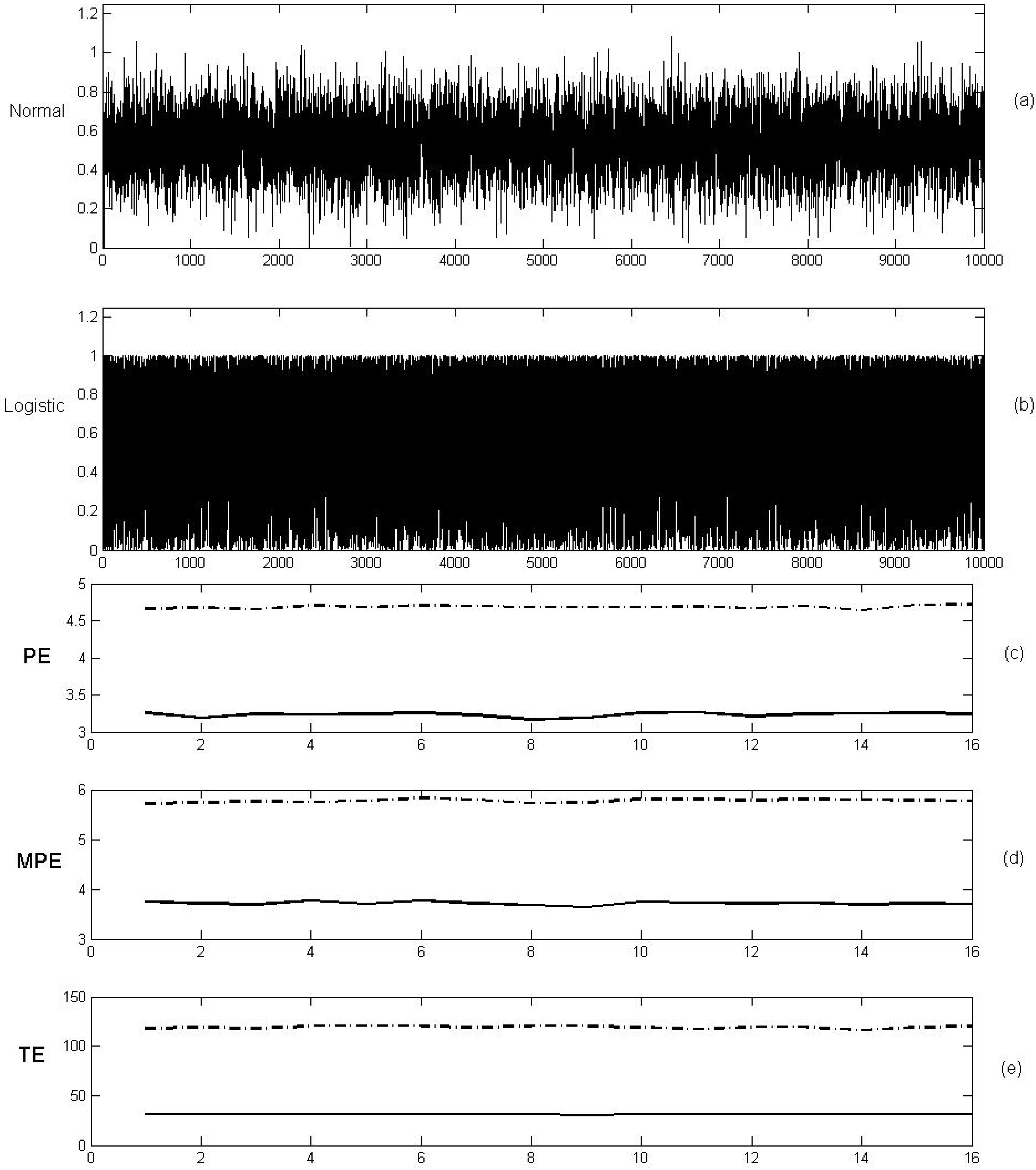
Figure 1 shows the PE, MPE and TE of both time series, using $m=5$ and $w=600$. For the Gaussian series, the number of admissible permutations in each sliding window is close to the maximum ($m!=5!=120)$, denoting a clear randomness of the data series. However, for the logistic series, the number of admissible permutations in each sliding window is 31 or below, denoting a deterministic behavior of this data series. Indeed, when a greater embedding dimension is used, $m=7$ and $w=10000=T$, it only appears as 178 different permutations of the $7!=5040$ possible in the logistic series, whereas the number of admissible permutations for the Gaussian series is 4348.

Figure 1. The (a) PE, (b) MPE and (c) TE of the two simulated time series ${(x_n)}_{n=1}^T$ and ${(y_n)}_{n=1}^T$, using $m=5$, $w=600$. Single lines correspond to the logistic map ${(y_n)}_n$ and the dotted lines correspond to the random series ${(x_n)}_n$.

Figure 1. The (a) PE, (b) MPE and (c) TE of the two simulated time series ${(x_n)}_{n=1}^T$ and ${(y_n)}_{n=1}^T$, using $m=5$, $w=600$. Single lines correspond to the logistic map ${(y_n)}_n$ and the dotted lines correspond to the random series ${(x_n)}_n$.

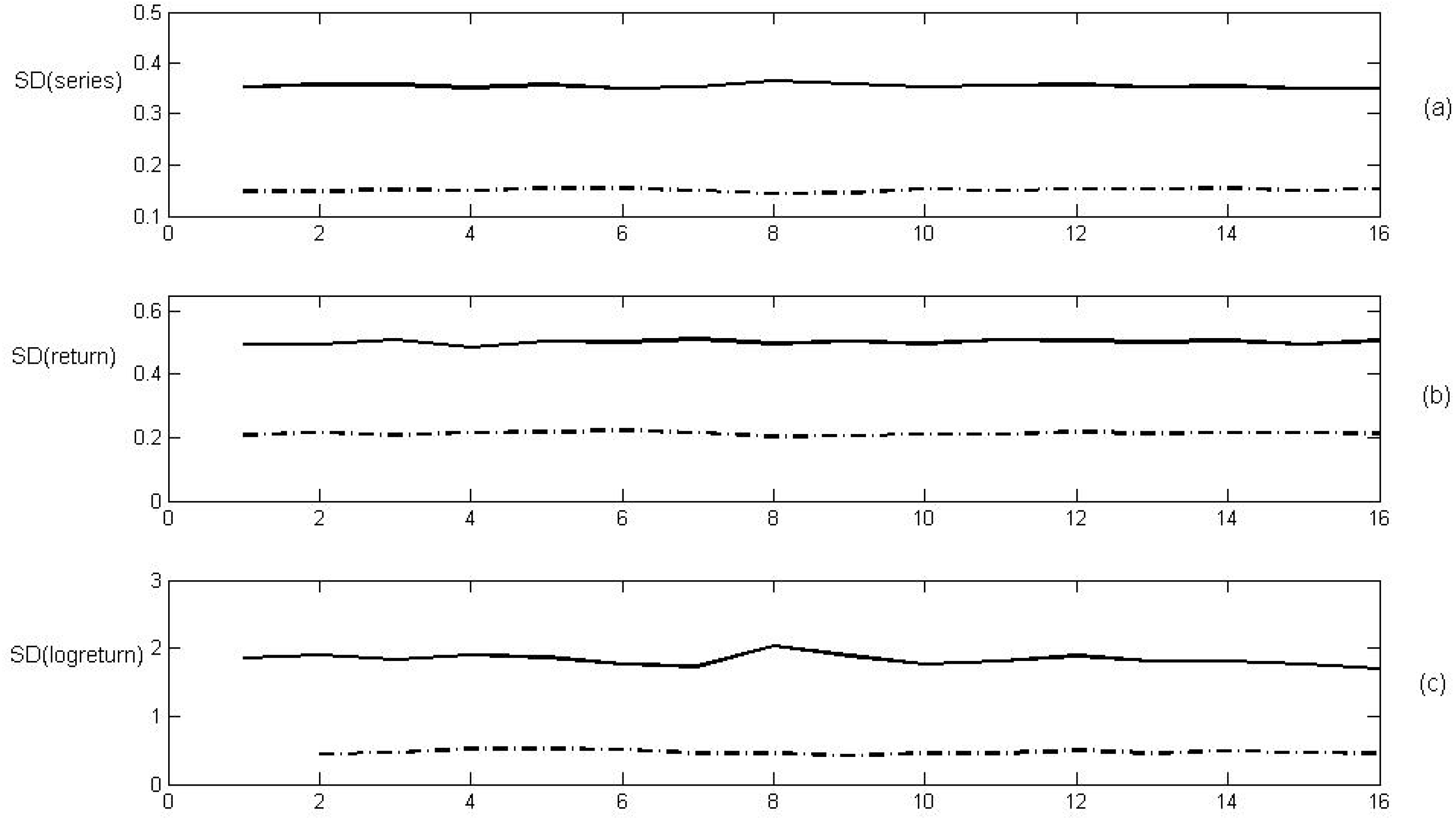
The situation changes when the common historical volatility measures are computed. Figure 2 shows three usual volatility measures corresponding to the standard deviation of : (1) the original time series, (2) the arithmetic return over a time period $h=1$, or (3) the logarithmic return over a time period $h=1$, for both simulated time series respectively. The length of the sliding window $w=600$ was chosen. For the three volatility measures, the Gaussian series provides lower volatility than the logistic map, which does not contemplate the actual degree or uncertainty of both simulated series.

Figure 2. The standard deviation of (a) the two simulated series, (b) their returns series and (c) their logarithmic return series. Single lines correspond to the logistic map ${(y_n)}_n$ and the dotted lines correspond to the random series ${(x_n)}_n$.

Figure 2. The standard deviation of (a) the two simulated series, (b) their returns series and (c) their logarithmic return series. Single lines correspond to the logistic map ${(y_n)}_n$ and the dotted lines correspond to the random series ${(x_n)}_n$.

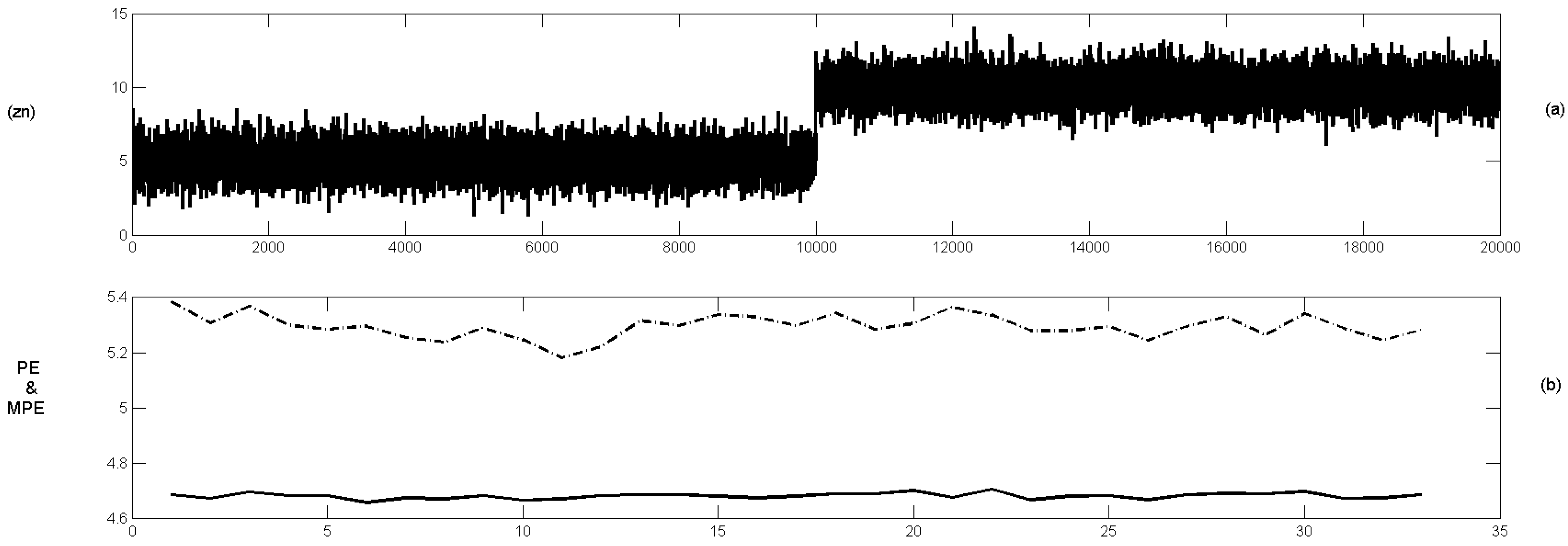
Note that the MPE shows greater differences than the PE between the degree of determinism of the two simulated series. Another example that reveals the utility of the MPE against the PE follows. Given that ${(u_n)}_{n=1}^T$ is an i.i.d. time series of size $T=5000$ generated by a Normal process with mean 0 and standard deviation 1 , and ${(v_n)}_{n=1}^T$ an i.i.d. time series of size $T=5000$ generated by a Normal process with mean 0 and standard deviation 4. Let ${(z_n)}_{n=1}^{2T}$ be the time series of size $2T=10000$ resulted in merging ${(u_n)}_{n=1}^T$ and ${(v_n)}_{n=1}^T$. Then, the PE of the series ${(z_n)}_{n=1}^{2T}$ remains almost constant along all sliding windows because both parts of the series have the same degree of uncertainty (they are both purely random). However, the features of both parts are quite different. The second part is “more volatile” than the first one because they have the same degree of uncertainty but the second part is more dispersed. This feature can be detected by computing the MPE, but not with the PE (see Figure 3).

Figure 3. The PE (single line) and MPE (dotted line) of the simulated time series ${(z_n)}_n$.

Figure 3. The PE (single line) and MPE (dotted line) of the simulated time series ${(z_n)}_n$.

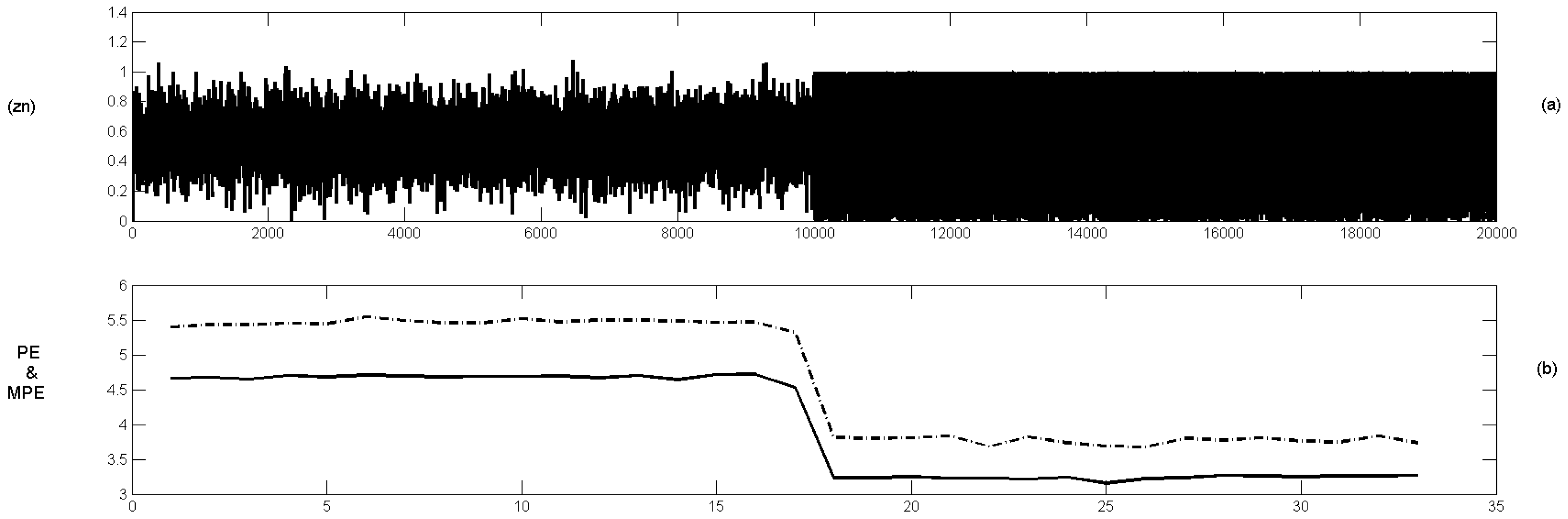
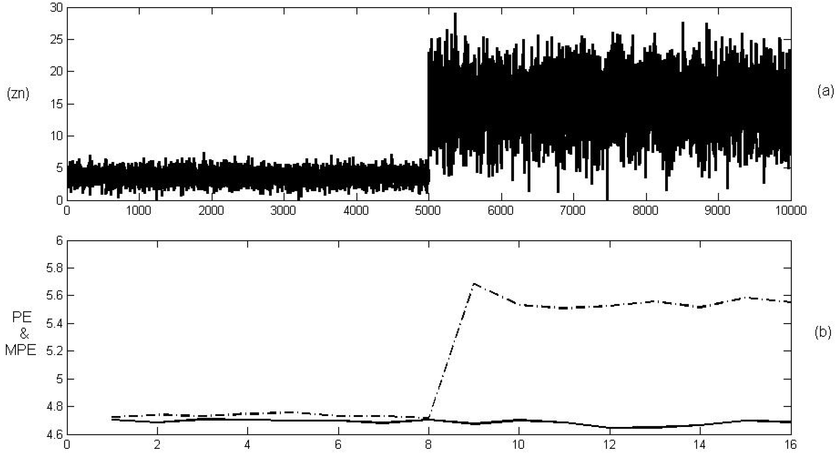
The proposed measures can identify “turning points” in terms of structural changes of the time series, namely, changes in the degree of uncertainty of the time series. However, they cannot detect changes in the level of the data series. For example, the following two situations are considered. Firstly, two merged Gaussian models with different means and the same standard deviation (pure randomness), and secondly, a Gaussian model merged into a Logistic map with similar means and standard deviations (randomness merged into determinism). The proposed measures do not detect the level change in the first case, but they can identify the structural change in the second case (see Figure 4 and Figure 5).

Figure 4. (a) The simulated time series ${(z_n)}_n$ resulted in merging two Gaussian processes with the same standard deviation ($\sigma =1$) and different means ($\mu =5$ and 10, respectively). (b) The PE (single line) and MPE (dotted line) of ${(z_n)}_n$ using $m=5$ and $w=600$.

Figure 4. (a) The simulated time series ${(z_n)}_n$ resulted in merging two Gaussian processes with the same standard deviation ($\sigma =1$) and different means ($\mu =5$ and 10, respectively). (b) The PE (single line) and MPE (dotted line) of ${(z_n)}_n$ using $m=5$ and $w=600$.

Figure 5. (a) The simulated time series resulted in merging the Gaussian processes and the logistic map given in Figure 1. (b) The PE (single line) and MPE (dotted line) of ${(z_n)}_n$ using $m=5$ and $w=600$.

Figure 5. (a) The simulated time series resulted in merging the Gaussian processes and the logistic map given in Figure 1. (b) The PE (single line) and MPE (dotted line) of ${(z_n)}_n$ using $m=5$ and $w=600$.

4. Applications to Some Energy Markets

In this section the proposed method is used to analyze the volatility of some of the representative electricity markets worldwide, such as Nord Pool, Ontario, the Spanish market (OMEL) and four of the Australian markets (NWS, QLD, SA, and VIC).

Moreover, the objective of this section is to show how the proposed volatility measures can detect the influence of “external” and “internal” factors on the unpredictability of electric energy prices. These results would enable regulators and market participants to learn and support the decisions taken in order to minimize their exposure to price volatility (in terms of price unpredictability) thus avoiding the inherent risk of long-term investments (for example, new generation or transmission capacity, or new efficient and expensive devices on the demand side).

The “external factors” are the ones which are not due to decisions or strategies made by electrical power system actors (generators, customers, distributors, commercializers, aggregators, system or market operators, etc.). For instance: the weather, regulatory acts, environmental constraints, the policies of neighboring markets (changing the flow of resources from one power system to another). On the contrary, the “internal factors” are due to policies implemented by the actors of a market. For instance, the activities of the power market, the capacity of energy storage, the mixture (diversity) of generation, the capacity margin change (generation vs. demand), the internal structure of the market (products and trade available on a short-term vs. medium-long term).

In this section the effect of some of the internal and external factors on price behavior and its volatility have been evaluated, as defined in the paper. First, the hourly spot prices in the Nordic electricity market (Nord Pool) in NOK/MWh for the period of May 4, 1992 to December 31, 1998 is considered. The spot prices in EUR/MWh from January 1, 1999 to December 31, 2009 are also taken into account. See [18]. The volatility of this power market was studied in [6,8], among others. The latter, proposed the DET and LAM variables associated to recurrence plots as alternative volatility measures. They based their analysis on known historical events: the evolution of the Nord Pool market and climatic factors.

According to the characteristics of the Nord Pool market, the volatility of prices could be influenced by different factors. The water reservoirs, because of its strong dependence on hydropower generation (nearly 47% of the total power generated in the Nord Pool market): Norway relies entirely on hydro, while Denmark generates all its power in thermal plants, mainly using imported coal. Sweden has a mixture of about half hydro and half nuclear generation, and Finland has a mixture of hydro (25%), conventional thermal (45%) and nuclear (30%). The amounts of bilateral contracts: since Nord Pool is not a mandatory pool, only a limited part of all power traded on the Nordic market is brokered there, and the rest is handled through bilateral contracts (at the beginning of 1996, Nord Pool’s market-share was about 10%, and by early 1999 it had risen to about 25% of all the power traded in Norway-Sweden). Changes in legislation: for example, the networks were gradually opened up to new players, and a new electricity act allowing a competitive market was finally implemented in January 1996 (entry of Sweden).

Table 1 summarizes the historical evolution of the Nord Pool, and Figure 6 provides the levels of the water reservoir (in percentages) from 1993 to 2009 (see [19,20]).

Table 1. Date of incorporation into the Nordic market (dd/mm/yy).

Countries	Date of entry
Norway	1/1/1993
Sweeden	1/1/1996
Finland	29/12/1997
West Denmark	1/7/1999
East Denmark	1/10/2000
KONTEK zone (Germany)	5/10/2005

Table 1. Date of incorporation into the Nordic market (dd/mm/yy).

Countries	Date of entry
Norway	1/1/1993
Sweeden	1/1/1996
Finland	29/12/1997
West Denmark	1/7/1999
East Denmark	1/10/2000
KONTEK zone (Germany)	5/10/2005

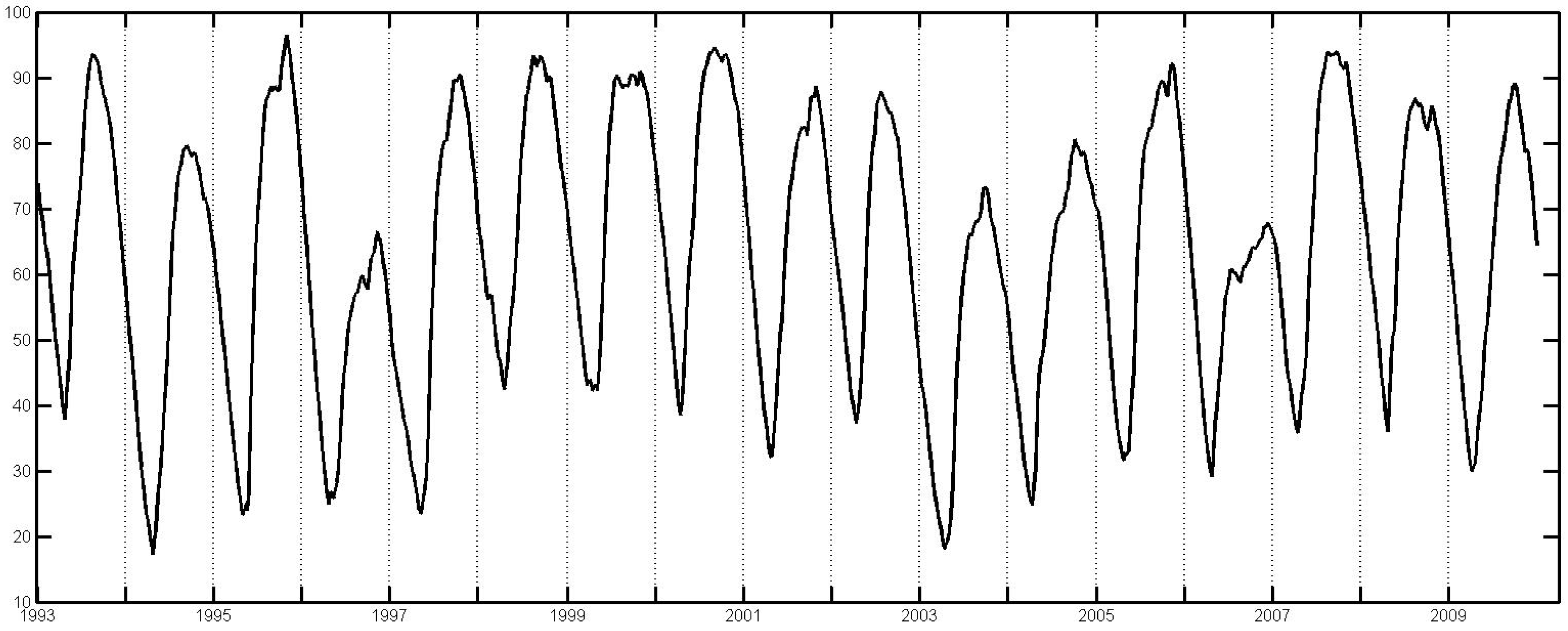
Figure 6. The water reservoir levels.

Figure 6. The water reservoir levels.

Note that 1994 and 2003 provided the lowest minimum reservoirs, whereas 1996, 2003 and 2006 registered the lowest maximum reservoirs: “1996 was a dry year and there was a sharp decline of precipitation during the autumn and winter season of 2002–2003”, as stated in [8].

Figure 7 and Figure 8 show the PE and MPE of the price data series when the embedding $m=5$ and sliding window $w=730$ are selected (note that $w=730$ hours approximately corresponds to one month). In addition, the mean of the PE and the MPE for each season (winter: from December 22 to March 20; spring: from March 21 to June 21; summer: from June 22 to September 23; autumn: from September 24 to December 21) have all been computed. In this last case, $m=5$ and $w=744$ were chosen and a little correction was made depending on the number of days of the season.

Note that results of the TE have been omitted in the rest of the paper due to their similarity to the PE.

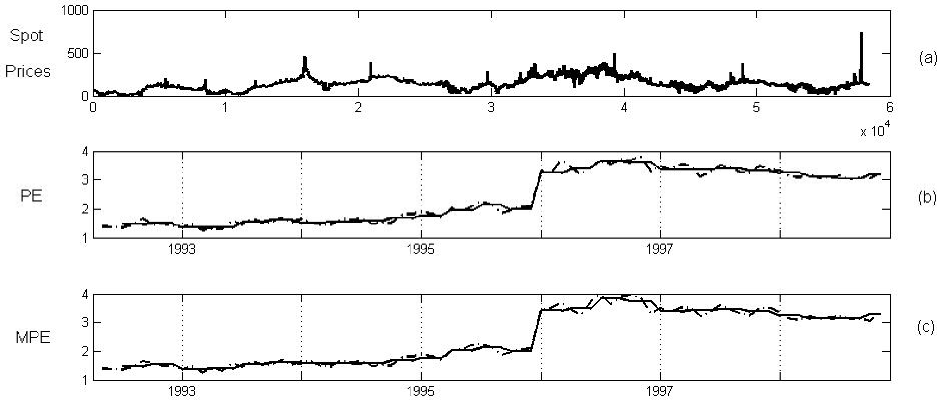
The PE and MPE show a weak increase at the end of 1994 and a sharp rise at the beginning of 1996, which was a dry year and when Sweden was incorporated into the market. However, both measures exhibit a smooth decrease during 1997 and 1998 (see Figure 5), which were wet years. Moreover, in these years, to reduce CO${}_2$ and NO${}_x$ emissions, the $2000MW$ of capacity (old fossil-fuel power plants) with the highest generation costs, was decommissioned in Sweden (see [21]).

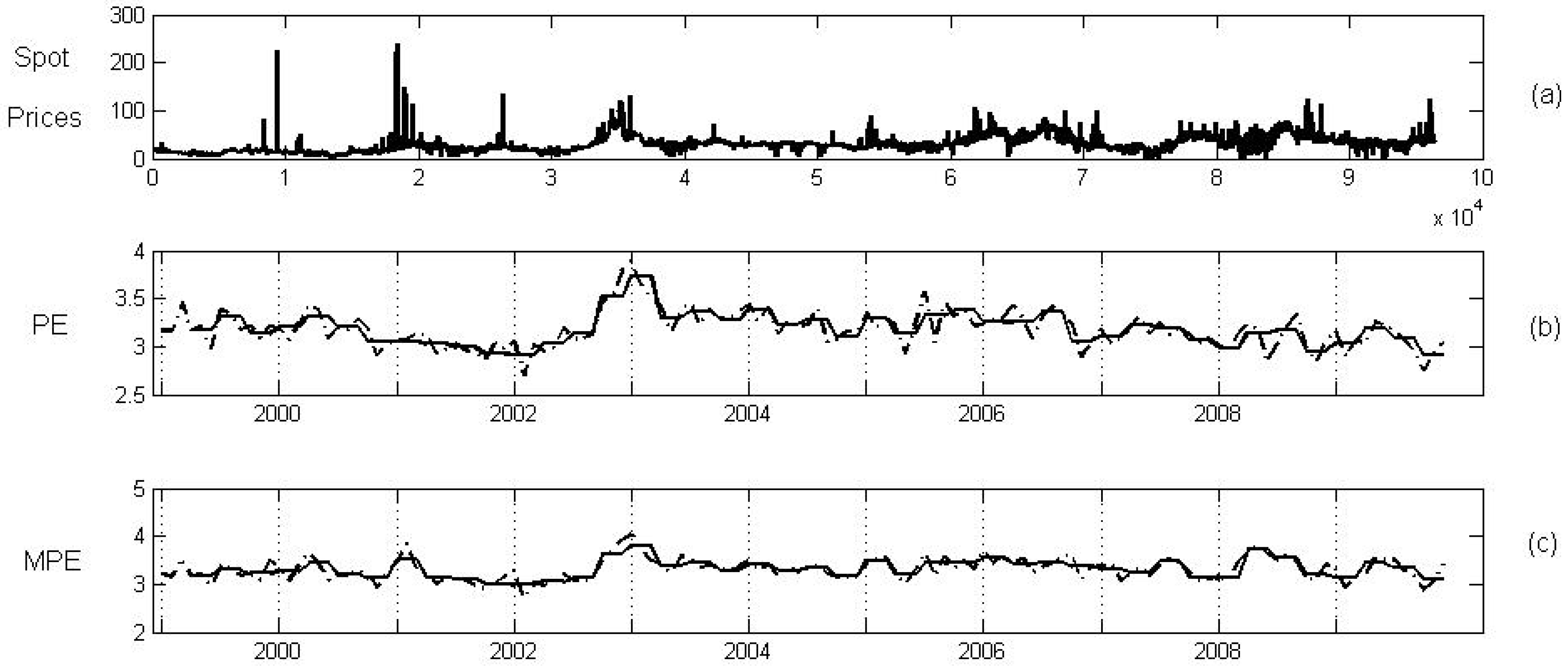
For the recent period, the highest PE and MPE appear in January–February 2003 (see Figure 6). This may be due to the sharp drop in precipitation during the autumn and winter season of 2002–2003.

In contrast, the MPE provides greater values (in average) when new countries are incorporated into the market, although the PE does not. For a more in-depth explanation of this, Table 2 shows the mean of the MPE and the mean of the PE for each period. Note that the highest mean corresponds to 1996, when different factors provoked a substantial increase in volatility.

In Figure 7 and Figure 8 please note that the PE and MPE do not seem to have annual cycles, even if the PE and MPE mean are calculated for each season. The lack of a seasonal behavior has been corroborated by means of the spectral analysis of the PE and MPE series and by computing their correlograms and partial correlograms.

Figure 7. (a) The Nord Pool spot prices from May 1992 to December 1998, in NOK/MWh. (b) The PE (dotted line) and its mean for each season (single line). (c) The MPE (dotted line) and its mean for each season (single line).

Figure 7. (a) The Nord Pool spot prices from May 1992 to December 1998, in NOK/MWh. (b) The PE (dotted line) and its mean for each season (single line). (c) The MPE (dotted line) and its mean for each season (single line).

Figure 8. (a) The Nord Pool spot prices from January of 1999 to December 2009, in EUR/MWh. (b) The PE (dotted line) and its mean for each season (single line). (c) The MPE (dotted line) and its mean for each season (single line).

Figure 8. (a) The Nord Pool spot prices from January of 1999 to December 2009, in EUR/MWh. (b) The PE (dotted line) and its mean for each season (single line). (c) The MPE (dotted line) and its mean for each season (single line).

Table 2. The mean of the MPE and PE in the periods determined by the incorporation of a new country.

Period	MPE mean	PE mean
From May 1992 to January 1993	1.47	1.45
From January 1993 to January 1996	1.70	1.68
From January 1996 to January 1997	3.53	3.43
From January 1997 to July 1999	3.19	3.15
From July 1999 to October 2000	3.29	3.23
From October 2000 to October 2005	3.30	3.20
From October 2005 to December 2009	3.35	3.13

Table 2. The mean of the MPE and PE in the periods determined by the incorporation of a new country.

Period	MPE mean	PE mean
From May 1992 to January 1993	1.47	1.45
From January 1993 to January 1996	1.70	1.68
From January 1996 to January 1997	3.53	3.43
From January 1997 to July 1999	3.19	3.15
From July 1999 to October 2000	3.29	3.23
From October 2000 to October 2005	3.30	3.20
From October 2005 to December 2009	3.35	3.13

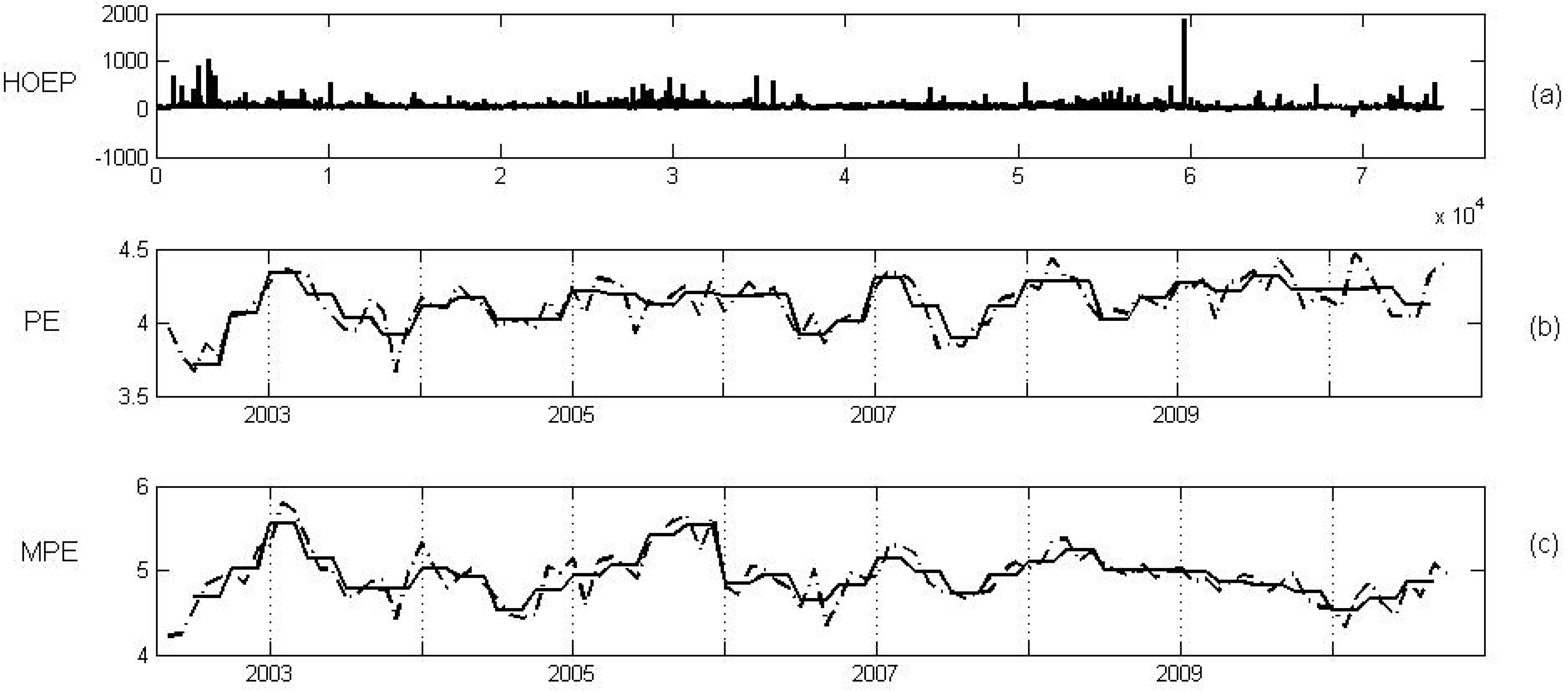
Secondly, the hourly Ontario energy price (HOEP) from May 1, 2002 to November 3, 2010 is taken into consideration (data available at [22]).

As mentioned previously in the introduction, [4] reported a study that quantifies price volatility for the Ontario and its neighboring electricity markets. The data used in the analysis were the historical HOEP for the period of May 1, 2002 to April 30, 2005, and the historical LMP data for 2004 on Ontario’s neighbors. The historical volatility was determined by taking into account the logarithmic returns with different time periods $h=1$, 24 and 168.

Figure 9 shows the HOEP data series and its corresponding PE and MPE when the embedding $m=5$ and the sliding window $w=730$ are selected (approximately one month). In addition, the mean of the PE and the MPE are computed for each season using $m=5$ and $w=744$.

The PE and MPE reveal certain seasonal behavior of a 12-month period during the 8 years analyzed. The seasonal behavior has been corroborated by using the spectral analysis of the PE and MPE series and by computing their correlograms and partial correlograms.

In general, summers provide lower volatilities and winters provide higher volatilities (except for the summer of 2009), perhaps because the differences between demand and the available generation are commonly greater in winters and lower in summers. Furthermore, Figure 9 shows that the highest HOEP volatility occurred in February and March 2003. Note that 2002–2003 was a year of change in the Ontario electricity market. Record temperatures in 2002–2003 brought record demands for electricity. At the same time, generation resource levels were lower than expected. Besides, a record in low water reservoirs conditioned hydroelectric generation and a number of environmental limitations affected the use of available generation through fossil fuel plants, all during periods of high demand. In the same year, the market price in Ontario attracted record amounts of generation from other jurisdictions (a growth of up to $33\%$ more in the volume of energy imports). The increase of volatility in this period is also in line with the statement in [4]: “the period of January, February and early March 2003 was an extremely cold period and natural gas prices were very high”. Finally, Figure 9 also reveals a change in the seasonal behavior for the previous two years analyzed (from summer 2008 to summer 2010), presenting a more stable entropy than the other years. This feature might be due to the influence of its neighboring markets: New York, New England and PJM which introduced the Capacity Markets at the end of 2007.

Figure 9. (a) The Ontario price series. (b) The PE (dotted line) and its mean for each season (single line). (c) The MPE (dotted line) and its mean for each season (single line).

Figure 9. (a) The Ontario price series. (b) The PE (dotted line) and its mean for each season (single line). (c) The MPE (dotted line) and its mean for each season (single line).

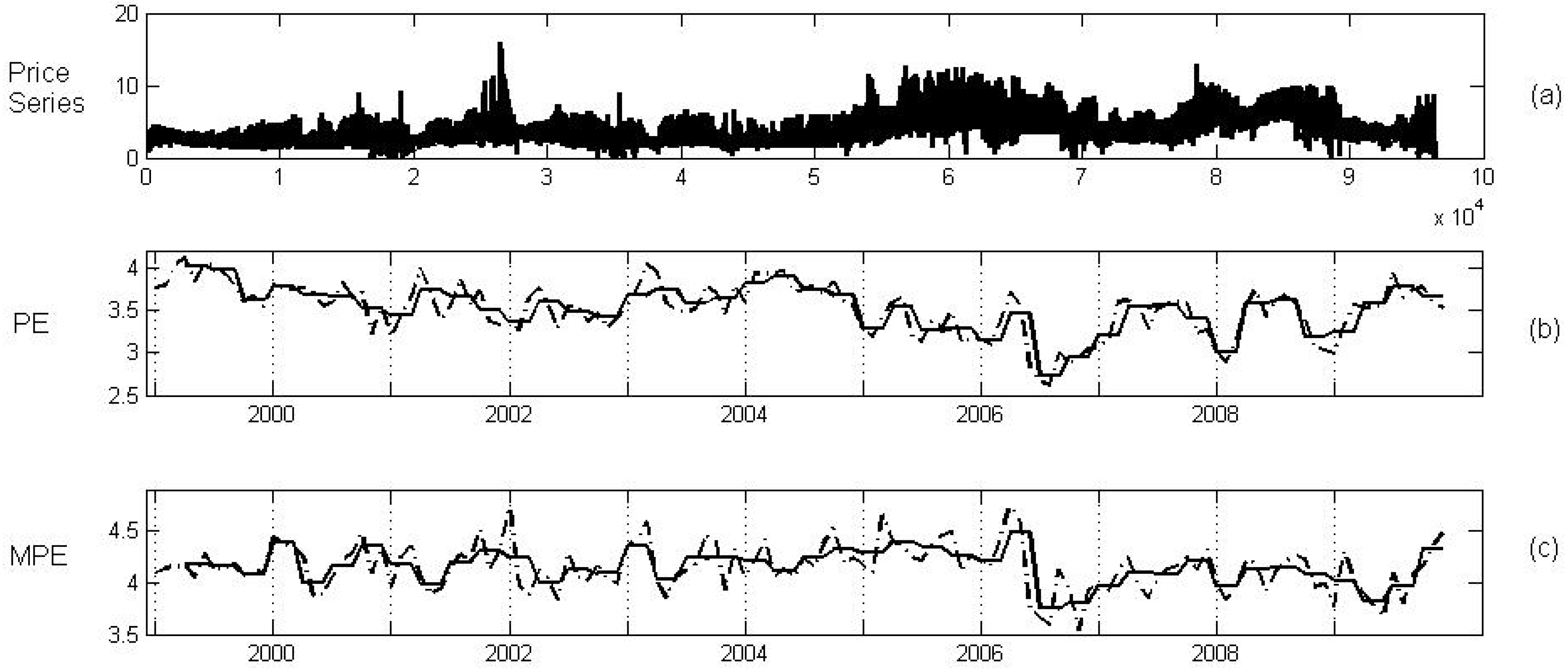
Thirdly, the hourly price data of the Spanish electricity market (OMEL) for 11 years, from January 1, 1999 to December 31, 2009 were considered.

The volatility of this power market was studied in [5], among others.

Figure 10 shows the price series and its corresponding PE and MPE when the embedding $m=5$ and the sliding window $w=730$ are selected (approximately one month). Again, the mean of the PE and the MPE for each season are computed using $m=5$ and $w=744$.

Figure 10. (a) The OMEL price series. (b) The PE (dotted line) and its mean for each season (single line). (c) The MPE (dotted line) and its mean for each season (single line).

Figure 10. (a) The OMEL price series. (b) The PE (dotted line) and its mean for each season (single line). (c) The MPE (dotted line) and its mean for each season (single line).

The PE and MPE show certain seasonal behavior, which becomes more evident when the mean for each season is computed. The spectral analysis reveals a seasonal behavior of a 12-month period in the case of PE and a 6 month period in the case of MPE. Note that usual climatic factors in Spain (cold winters and very hot summers) are also in line with half-year cycles.

To explain the volatility of this market in greater detail, the fact that Spain and Portugal are almost like an island from an electrical point of view should be contemplated. It is worth mentioning that the electrical interconnection with France is below $5\%$ of the peak demand in Spain. In contrast, since 2005, new regulations, namely the Spanish Royal Act 3/2005 [23], have tried to improve competitiveness in distribution and generation levels as well as the transparency of the market. Moreover, attempts have been made to reduce the risk of some of the actors pressurizing the power market. Besides, in the Spanish market most of the trade took place through the day ahead market until spring of 2006, when new regulations and acts [24] shifted a significant amount of trade over to adjustment markets (see [25]). One example that is partly due to these acts, is that nearly $23\%$ of energy trades changed from the day ahead and intradaily energy markets to bilateral contracts (2006), because price caps were lower than market prices [26].

Finally, the price data series of four Australian markets are analyzed: New South Wales (NSW), Queensland (QLD), South Australia (SA) and Victoria (VIC). The National Electricity Market of Australia (NEM) is an interconnected grid consisting of several connected regional networks. The NEM operates across the eastern states of the mainland. Each state region (subsystems) publishes a half-hourly spot pool price for electricity based on a gross pool merit order dispatch system. The data correspond to half-hourly electricity prices, from January 1, 2004 to December 31, 2009 (data available at [27]). The volatilities of these power markets were studied in [5] using the concept of price velocity for the period from December 13, 1998 to December 31, 2001.

Figure 11 shows the PE of the four price series with embedding $m=5$ and sliding window$w=1460$ ($w=1460$ corresponds to one month, approximately). The mean of the PE for each season is also reported. Results using the MPE are nearly identical to those using the PE, therefore these have been omitted.

Figure 11. (a) The PE of the four price series. (b) The mean of the PE for each season.

Figure 11. (a) The PE of the four price series. (b) The mean of the PE for each season.

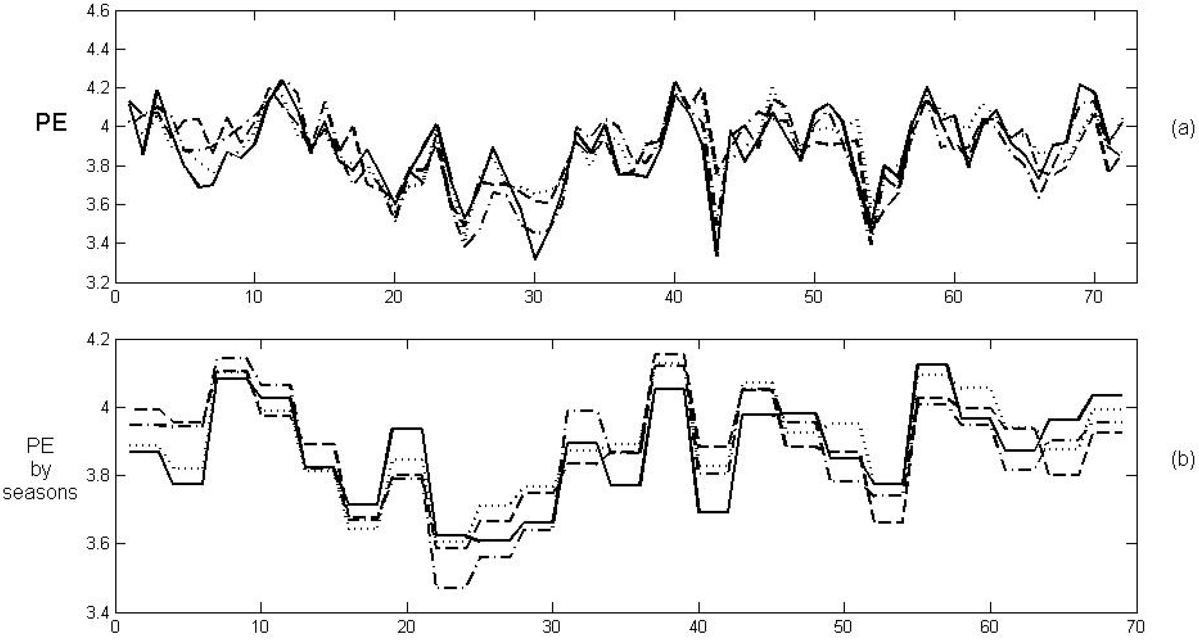
The PE show a seasonal behavior of a 12-month period, which has been corroborated again by spectral analysis.

The PE exhibits low volatilities in summers and high volatilities in autumns. The lowest volatility in the four Australian markets is seen to be in summer 2006.

Please note that the four Australian markets provide very similar PE patterns, revealing a strong dependence among the volatilities of these electricity markets.

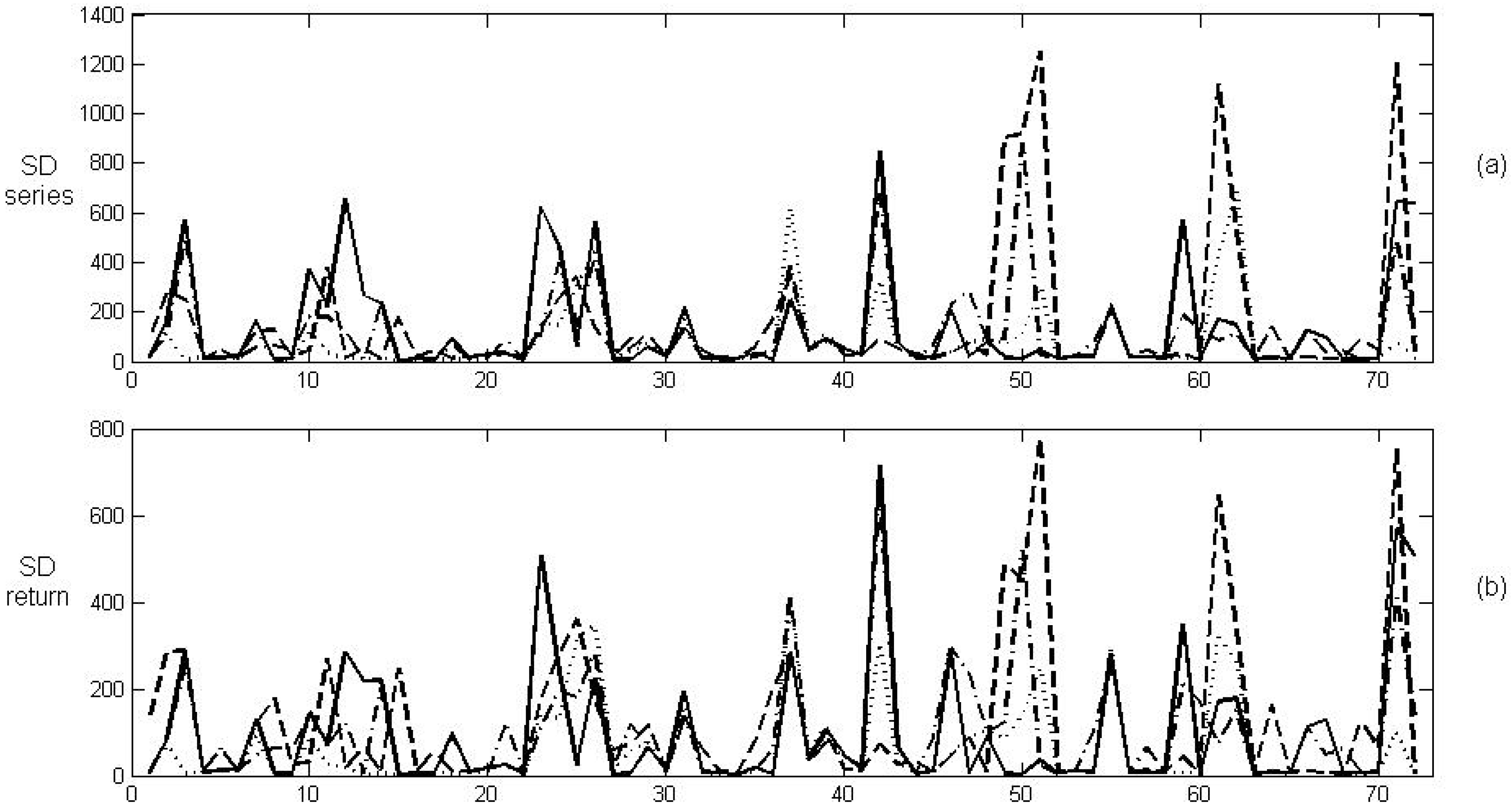
This behavior corresponds to a multi-regional market that works as a gross pool with 6 nodes in a Locational Marginal Price structure (LMP) for each zone (each zone usually corresponds to a state). However, Figure 12 shows that this dependence feature cannot be detected so clearly through the common historical volatility measures (standard deviation of the series or its returns, when $w=1460$ is chosen).

Figure 12. (a) The standard deviation of the four price series. (b) The standard deviation of their return series.

Figure 12. (a) The standard deviation of the four price series. (b) The standard deviation of their return series.

Indeed, the cross-correlation analysis for the PE’s provides $0.871$ as the maximum value of correlation between NSW and QLD, which corresponds to lag 0. However, if the common volatility measures (standard deviation) is used, the cross-correlation analysis provides $0.4$ as the maximum correlation between NSW and QLD, which also corresponds to lag 0. Moreover the cross-correlation analysis of the PE’s reveals a strong association between SA and VIC (correlation Pearson $=0.863$).

Therefore, using the PE (TE or MPE) as a volatility measure, the associations among different power markets can be identified, as previously shown for the Australian markets. In this context, the possible relationship of volatilities of the electricity markets analyzed (Nord Pool, Ontario, OMEL and Australian’s) has also been studied. Whereby, a common period of time for all markets has been used that ranges from January 2004 to December 2009. The cross-correlation analysis reveals that neither Nord Pool nor Ontario are related to any of the other markets. However, the association between OMEL and the Australian markets is weak, with the maximum correlation $0.546$ corresponding to lag 6 months (this may be due to similar climatic factors and the differences between seasons in the northern and southern hemispheres).

In Table 3, a ranking of the power markets analyzed is shown according to their mean volatilities in the common period from January 2004 to December 2009. Ontario provides the highest volatility, followed by the Australians and OMEL, whereas Nord Pool provides the lowest volatility. This ranking is in line with [5].

Table 3. The mean of the PE and MPE for each market, from 2004 to 2009.

Market	PE mean	MPE mean
Ontario	4.14	4.95
VIC	3.89	3.95
SA	3.88	3.92
NSW	3.87	3.93
QLD	3.87	3.93
OMEL	3.41	4.13
Nord Pool	3.16	3.34

Table 3. The mean of the PE and MPE for each market, from 2004 to 2009.

Market	PE mean	MPE mean
Ontario	4.14	4.95
VIC	3.89	3.95
SA	3.88	3.92
NSW	3.87	3.93
QLD	3.87	3.93
OMEL	3.41	4.13
Nord Pool	3.16	3.34

5. Conclusions

In this paper, the Permutation Entropy, Topological Entropy and the Modified Permutation Entropy are proposed as alternative volatility measures, instead of common historical volatility measures which are computed through the standard deviation. Simulated data show that these proposed measures are appropriate to quantify the degree of randomness or determinism of a time series, so as to measure volatility. Furthermore, no assumption is needed to compute the volatility and the existing nonlinear dynamic in price series data can be taken into account too.

Applying our method to some electricity markets shows the capacity of the new measures to relate periods with high and low volatilities to historical events or climatic factors. Besides, some interesting features such as the seasonal behavior of the volatilities or associations among markets can also be detected using these entropy measures.

Therefore, the proposed measures help to identify the factors that can produce changes in the predictability of the price series (such as loads, climatic factors, market regulations, etc.). Moreover, they can identify the time periods with a high degree of determinism and find out whether seasonal behavior exists. For example, they could determine that summers are less volatile than the rest of the seasons, and this fact would be applied to improve forecasting price models. The proposed volatility measures might also be useful to compare the uncertainty associated with different commodities (electricity, oil, gas, etc.), to determine which of them is more predictable. Finally, the volatility of the prices provides investors, customers and regulators with important feedback.

References

- Henning, B.; Sloane, M.; de Leon, M. Natural gas and energy price volatility. American Gas Foundation 2003. Available online: http://www.gasfoundation.org/ResearchStudies/VolStudyCh5.pdf (accessed on 19 January 2012).
- Newell, S.; Bhattacharyya, A. Cost-benefit analysis of replacing the NYISO’s existing ICAP market with a forward capacity market. The Brattle Group Inc., 2009. Available online: http://www.brattle.com/_documents/UploadLibrary/Upload789.pdf (accessed on 19 January 2012).
- Benini, M.; Marracci, M.; Pelacchi, P.; Venturini, A. Day-ahead market price volatility analysis in deregulated electricity markets. In Proceedings of the IEEE Power Engineering Society Summer Meeting, Chicago, IL, USA, 25 July 2002; Volume 3, pp. 1354–1359.
- Zareipour, H.; Bhattacharya, K.; Canizares, C. Electricity market price volatility: The case of Ontario. Energy Policy 2007, 35, 4739–4748. [Google Scholar] [CrossRef]
- Li, Y.; Flynn, P.C. Deregulated power prices: Comparison of volatility. Energy Policy 2004, 32, 1591–1601. [Google Scholar] [CrossRef]
- Simonsen, I. Volatility of power markets. Phys. Stat. Mech. Appl. 2005, 335, 10–20. [Google Scholar] [CrossRef]
- Regnier, E. Oil and energy price volatility. Energ. Econ. 2007, 29, 405–427. [Google Scholar] [CrossRef]
- Strozzi, F.; Gutierrez, E.; Noe, C.; Rossi, T.; Serati, M.; Zaldivar, J.M. Measuring volatility in the nordic spot electricity market using recurrence quantification analysis. Eur. Phys. J. 2008, 164, 105–115. [Google Scholar] [CrossRef]
- Perello, J.; Montero, M.; Palatella, L.; Simonsen, I.; Masoliver, J. Entropy of the Nordic electricity market: Anomalous scaling, spikes, and mean reversion. J. Stat. Mech. Theor. Exp. 2006, 11, P11011. [Google Scholar] [CrossRef]
- Amjady, N.; Keynia, F. Day ahead price forecasting of electricity markets by mutual information technique and cascaded neuro evolutionary algorithm. IEEE Trans. Power Syst. 2009, 24, 306–318. [Google Scholar] [CrossRef]
- Cao, Y.H.; Tung, W.W.; Gao, J.B.; Protopopescu, V.A.; Hively, L.M. Detecting dynamical changes in time series using the permutation entropy. Phys. Rev. E 2004, 70, 046217. [Google Scholar] [CrossRef]
- Bruzzo, A.A.; Gesierich, B.; Santi, M.; Tassinari, C.A.; Birbaumer, N.; Rubboli, G. Permutation entropy to detect vigilance changes and preictal states from scalp EEG in epileptic patients. A preliminary study. Neurol. Sci. 2008, 29, 39–45. [Google Scholar] [CrossRef] [PubMed]
- Canovas, J.S. Estimating topological entropy from individual orbits. Int. J. Comput. Math. 2009, 86, 1901–1906. [Google Scholar] [CrossRef]
- Canovas, J.S.; Guillamon, A. Permutations and time series analisys. Chaos 2009, 19, 043103. [Google Scholar] [CrossRef] [PubMed]
- Canovas, J.S.; Guillamon, A.; Ruiz, M.C. Using permutations to find structural changes in time series. Fluctuation and Noise Letters 2011, 10, 13–30. [Google Scholar] [CrossRef]
- Bandt, C.; Pompe, B. Permutation entropy: A natural complexity measure for time series. Phys. Rev. Lett. 2002, 88, 174102. [Google Scholar] [CrossRef] [PubMed]
- Liu, X.; Wang, Y. Fine-grained permutation entropy as a measure of natural complexity for time series. Chin. Phys. B 2009, 18, 2690–2696. [Google Scholar]
- Nord Pool Spot. Available online: http://www.nordpoolspot.com (accessed on 19 January 2012).
- Nord Pool Reservoir Data. Available online: http://www.nordpoolspot.com/Market-data1/Power-system-data/Hydro-Reservoir/ (accessed on 19 January 2012).
- Statistics Norway. Available online: http://www.ssb.no/vannmag_en/tab-01-en.shtml (accessed on 19 January 2012).
- Bhattacharya, K.; Bollen, M.H.J.; Daalder, J.E. Operation of Restructured Power Systems; Kluwer Academic Publishers: Boston, MA, USA, 2001. [Google Scholar]
- Independent Electricity System Operator of Ontario Market. Available online: http://www.theimo.com/imoweb/marketdata/marketData.asp (accessed on 19 January 2012).
- Boletin Oficial del Estado (BOE) (Official State Gazette). Real Decreto (Royal Decree) 5/2005 (in Spanish); BOE no. 62, 8832-8853 March 2005. Available online: http://www.boe.es (accessed on 19 January 2012).
- Boletin Oficial del Estado (BOE) (Official State Gazette). Real Decreto (Royal Decree) 3/2006 (in Spanish); BOE no. 150, 8015-8016, February 2006. Available online: http://www.boe.es (accessed on 19 January 2012).
- Conejo, A. The electricity market of mainland Spain: A brief critical review. In Proceedings of the IEEE Power Engineering Society General Meeting, Tampa, FL, USA, 24–28 June 2007.
- Electricity Market of Spain. 2006 Annual Report, OMEL market operator. Available online http://www.omie.es/files/me06cast.pdf (accessed on 19 January 2012).
- Australian Energy Market Operator. Available online: http://www.aemo.com.au/data/price_demand.html (accessed on 19 January 2012).
© 2012 by the authors; licensee MDPI, Basel, Switzerland. This article is an open access article distributed under the terms and conditions of the Creative Commons Attribution license (http://creativecommons.org/licenses/by/3.0/).
Share and Cite
MDPI and ACS Style
Ruiz, M.d.C.; Guillamón, A.; Gabaldón, A. A New Approach to Measure Volatility in Energy Markets. Entropy 2012, 14, 74-91. https://doi.org/10.3390/e14010074
AMA Style
Ruiz MdC, Guillamón A, Gabaldón A. A New Approach to Measure Volatility in Energy Markets. Entropy. 2012; 14(1):74-91. https://doi.org/10.3390/e14010074
Chicago/Turabian StyleRuiz, María del Carmen, Antonio Guillamón, and Antonio Gabaldón. 2012. "A New Approach to Measure Volatility in Energy Markets" Entropy 14, no. 1: 74-91. https://doi.org/10.3390/e14010074