1. Introduction
Time series (TS) data originating from different physical/natural systems/processes usually contain extremely valuable information. Traditionally, such information is conveyed in the form of probabilistic distribution functions (PDFs) that, in some sense, represent the TS. The problem we discuss is how to best extract that information from the time series. This, of course, is tantamount to asking for the best PDF that represents it. The indirect data always possess a stochastic component due to the omnipresent dynamical noise [
1,
2]. Consequently, the specific procedure one employs in extracting a TS from given data seriously affects the quality of the information one may gain.
To study this the extraction issue is the purpose of this paper. To do this we consider two popular PDF extraction methodologies and analyze their information-content. Then we introduce a basis to quantitatively assess the amount of information a PDF contains.
The extraction procedures are considered in
Section II.
Section III is devoted to the CR-divergence family of entropic functionals. Two scenarios that will serve as applications are described in
Section IV and results are presented
Section V. Finally, some conclusions are drawn in
Section VI.
2. Two Popular Extraction Procedures
In this Section we generate an appropriate time-series (TS) and proceed to extract from it a suitable PDF. The crucial issue is getting the “best” PDF that will properly “capture” either the physics at hand, the nature of the associated underlying natural process, and/or the features of the TS-generating nonlinear dynamical system. Two methodologies have become popular in this respect and we describe them in the subsections below.
2.1. PDF Based on Histograms
In order to extract a PDF via amplitude-statistics, the interval (with a and b the minimum and maximum of the time series ) is first divided into a finite number of non-overlapping subintervals : and . One then employs the usual histogram-method, which is based on counting the relative frequencies of the time series values within each subinterval.
It should be clear that the resulting PDF lacks any information regarding temporal ordering (temporal causality). The only pieces of information that result are the
values that allow one to assign inclusion within a given bin, thus ignoring the temporal order (this is, the subindex
t). In addition, it is necessary to consider a judiciously chosen optimal value for
(see De Micco
et al. [
3]).
2.2. PDF Based on Bandt and Pompe’s Methodology
To use the Bandt and Pompe [
4] methodology for evaluating the probability distribution
P associated with the time series (dynamical system), one starts by considering partitions of the pertinent
D-dimensional space that will hopefully “reveal" relevant details of the ordinal structure of a given one-dimensional time series
with embedding dimension
and time delay
τ. In the following we take
as the time delay [
4]. We are interested in “ordinal patterns", of order
D [
4,
5], generated by
which assigns to each time
s the
D-dimensional vector of values at times
. Clearly, the greater the
value, the more information on the past is incorporated into our vectors. By “ordinal pattern" related to the time
, we mean the permutation
of
defined by
In order to get a unique result we set , if . This is justified if the values of have a continuous distribution so that equal values are very unusual. Otherwise, it is possible to break these equalities by adding small random perturbations.
Thus, for the
possible permutations
π of order
D, the associated relative frequencies can be naturally computed by the number of times this particular order sequence is found in the time series divided by the total number of sequences. The probability distribution
is defined by
In this expression, the symbol ♯ stands for “number".
The procedure can be illustrated with a simple example; let us assume that we start with the time series
, and we set the embedding dimension
. In this case the state space is divided into
partitions and 24 mutually exclusive permutation symbols are considered. The first 4-dimensional vector is
. According to Equation (
1) this vector corresponds with
. Following Equation (
2) we find that
. Then, the ordinal pattern that allows us to fulfill Equation (
2) will be
. The second 4-dimensional vector is
, and
will be its associated permutation, and so on. For the computation of the Bandt and Pompe PDF, we follow the very fast algorithm described by Keller and Sinn [
6], in which the different ordinal patterns are generated in lexicographic ordering.
The Bandt–Pompe methodology is not restricted to a time series (TS) representative of low dimensional dynamical systems. It can be applied to any TS-type (regular, chaotic, noisy, or reality based), with a very weak stationary assumption. This means the probability of finding
should not depend on
t [
4]). It is assumed that enough data are available for a correct embedding procedure, of course. The embedding dimension
D plays an important role in the evaluation of the appropriate probability distribution, because
D determines the number of accessible states
. The minimum acceptable length of the time series that one needs in order to extract reliable statistics is
.
3. Quantifier of a PDF’s Information Content: the CR Divergence Measure
Our goal is to assess the informational content of the two methodologies reviewed above. To this end we will use, following Judge and Mittelhammer [
7], the Cressie–Read family of divergence measures [
8]. This family of divergence measures provides us with an objective assessment of how much information a given PDF contains relative to a second PDF. In this sense, CR-divergences are extensions of the celebrated Kullback–Leibler divergence. For two normalized, discrete probability distribution functions (PDF)
p and
q, one has [
8]
where
γ is a parameter that indexes members of the CR family, and the
represent the subject probabilities. The
’s are interpreted as reference probabilities. Being probabilities, the usual PDF characteristics of
for all
i are assumed. The CR family of power divergences is defined through a class of additive convex functions and the CR power divergence measure encompasses a broad family of test statistics that leads to a broad family of likelihood functions within a moments-based estimation context. In an extremum metrics scenario, the general Cressie-Read family of power divergence statistics represents a flexible family of pseudo-distance measures from which to derive empirical probabilities associated with indirect noisy micro and macro data [
8].
As
γ varies, the resulting estimators that minimize power divergence exhibit qualitatively different sampling behavior. As an illustration, a solution to the stochastic inverse problem, (for any given choice of the parameter) may be formulated by recourse to empirical sample moments (as constraints) [
9].
To place the CR family of power divergence statistics in an entropic perspective, we note that there are corresponding Renyi and Tsallis families of entropy functionals-divergence measures [
10]. As demonstrated by Gorban
et al. [
9], over defined ranges of the divergence measures, the CR and entropy families are equivalent. Relative to Renyi and Tsallis, the CR family has a more convenient normalization factor
, and has proper convexity for all powers, both positive and negative. The CR family has the separation of variables for independent subsystems [
9] over the range of
γ. This separation of variables permits the partitioning of the state space and is valid for divergences in the form of a convex function. In this preliminary illustrative effort we use
.
3.1. The Information We Seek to Gain
The family of CR-divergences gives us an essential piece of information. Given two PDFs p and q, permits us to determine what new information is contained in p relative to that contained in q. If q is a uniform PDF, it conveys no information and I measures the information content of p. In the present analysis p will be associated with the Bandt–Pompe PDF and q with the histogram procedure.
3.2. Three Main Variants of
Three discrete CR alternatives for , where , have received the most attention, empirically and in the literature, to date. In reviewing these, we adopt the notation , where the arguments p and q are tacitly understood to be evaluated at relevant vector values. In the two special cases where or , the notation and are to be interpreted as the continuous limits, or , respectively.
In the discrete instance in which the PDFs have n components, we let q be the uniform distribution , the reference distribution q is the empirical distribution function (EDF) associated with the observed sample data.
The Kullback–Leibler divergence is easily seen to emerge if we set , while if we set we get the KL .
Minimizing is then equivalent to maximizing and leads to the traditional maximum empirical log-likelihood (MEL) objective function. Minimizing is equivalent to maximizing , and leads to the maximum empirical exponential likelihood (MEEL) objective function, which is also equivalent to Shannon’s entropy. Finally, minimizing is equivalent to maximizing , and leads to the maximum log-Euclidean likelihood (MLEL) objective function. Note the latter objective function is also equivalent to minimizing the sum of squares function, in self-explanatory notation.
5. Results
We present in this section our main results regarding the two systems under scrutiny here.
5.1. CR-Results for the Logistic Map
In
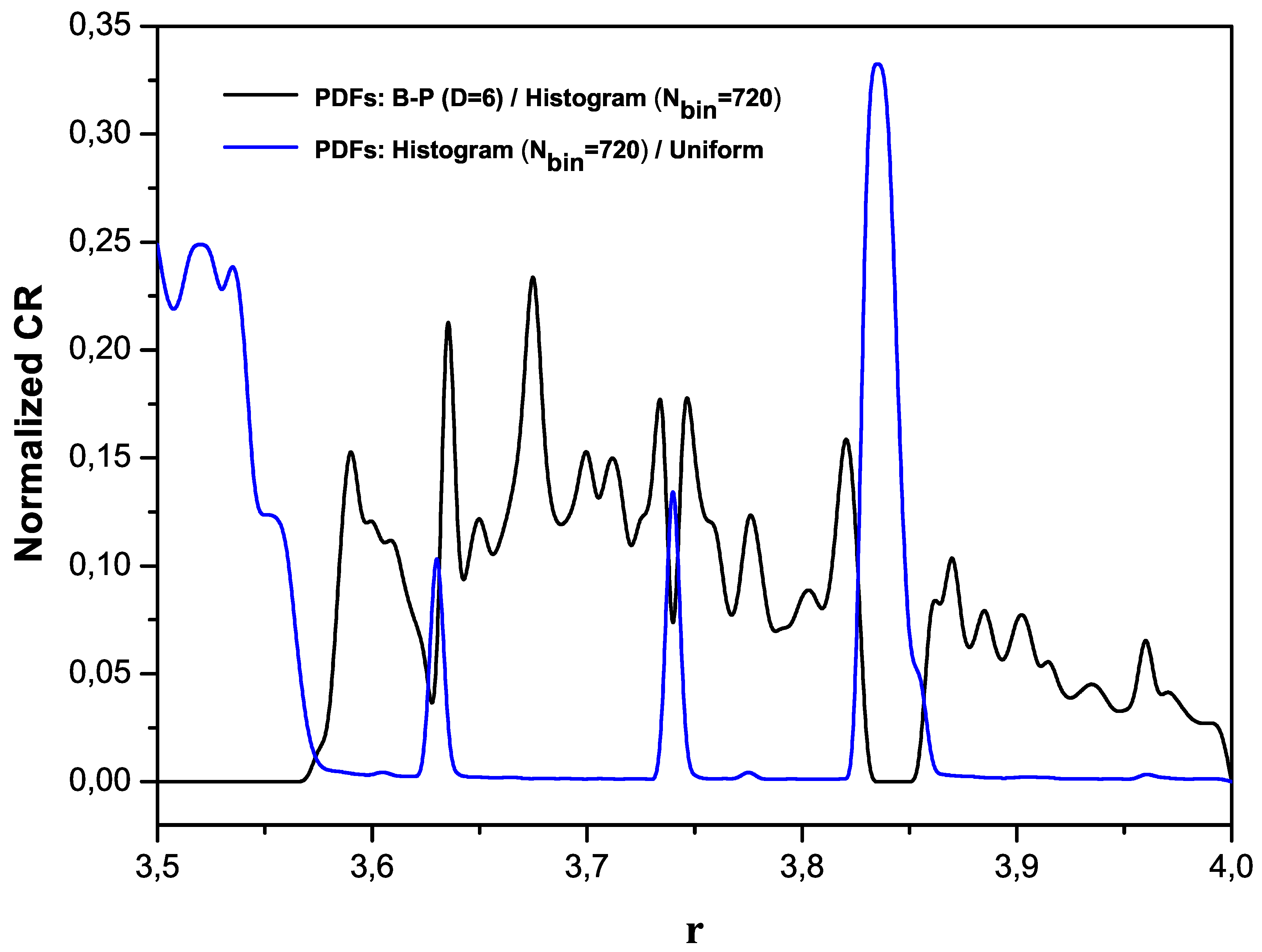
Figure 2, we compare three different PDFs. One is obtained using the histogram technique, another pertains to the BP methodology, and, for the sake of easy reference, we include the uniform PDF, that conveys no information at all.
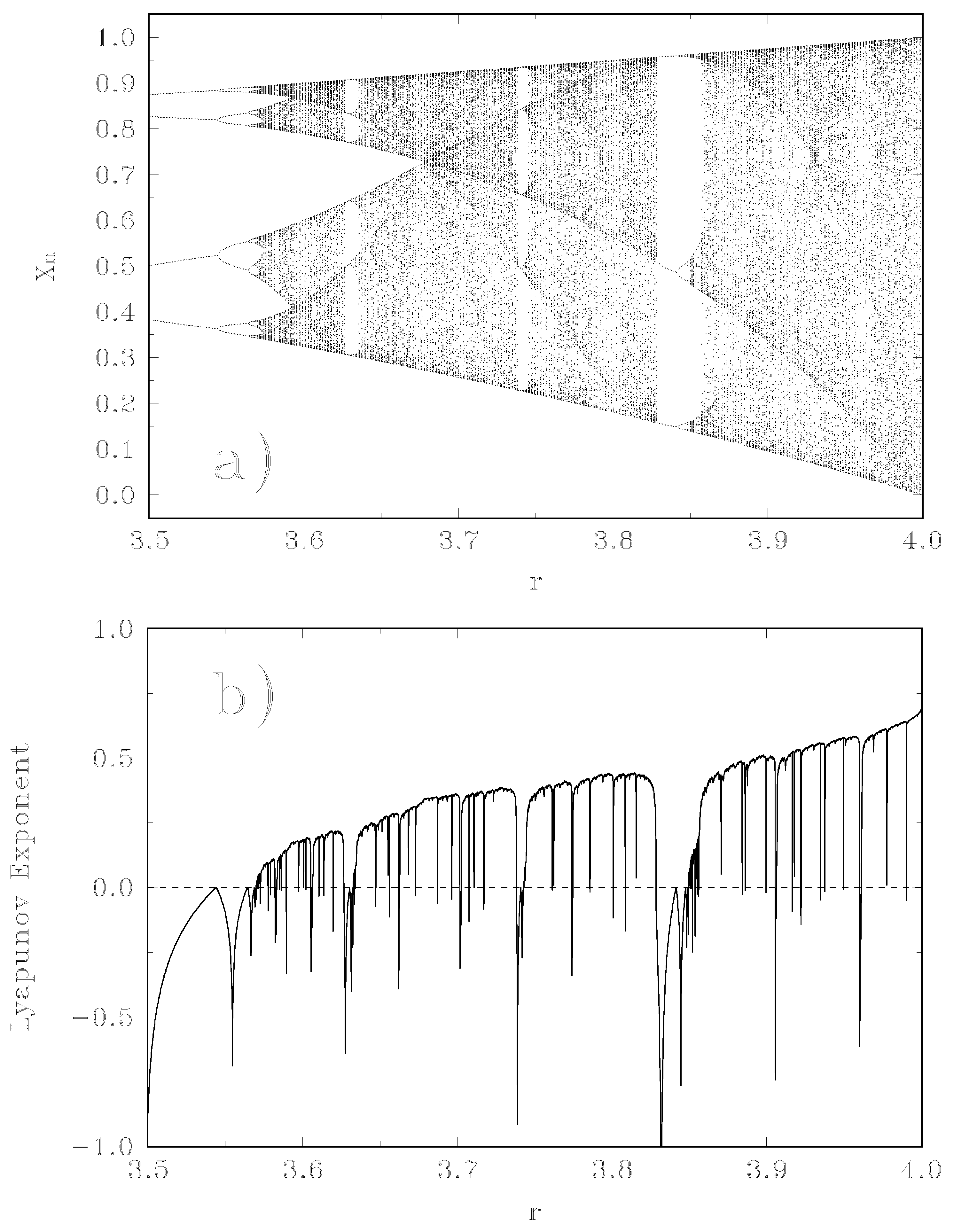
(1) At , cycles of period 2, 4, 8, 16, 32, … appear and we have chaos at , which is clearly displayed in the graph. The histogram results greatly differ from the “uniform-PDF" (blue line), which suggests that its information-content is significant. Notice that the BP line (black) is zero at the periodic windows. This is easily understood, since temporal causality (the important BP feature) is irrelevant for periodic motion.
(2) In the interval chaos reigns: now causality and ordinal patterns become of the essence. The time-series values for these values exhibit an almost uniform distribution. This means that the histogram PDF does not yield any information not possessed by the uniform PDF (blue line at zero)! This kind of behavior repeats itself as chaotic windows and periodic ones alternate one after the other, and the graph clearly depicts this effect. Intermittent behavior near the beginning and the end of a periodic window is also detected and the histogram and BP lines are different form zero. The histogram-technique “acquires" extra-information over the uniform PDF, whenever order prevails. Alternatively, when chaos prevails, BP gains information over histograms. With the above reported results in mind, we now turn to a physical scenario.
Figure 2.
I(B-P,histogram,1) and I(histogram,uniform,1) for the logistic map as a function of the parameter r.
Figure 2.
I(B-P,histogram,1) and I(histogram,uniform,1) for the logistic map as a function of the parameter r.
5.2. CR-physical Results
Signal
vs. time graphs pertaining to the physical model are presented in
Figure 3. Subplots 1–5 refer to solutions of the system Equation (
8) (semi-quantum signal), for representative fixed values of
. Subplots 6–10 refer to solutions of the classical counterpart of the system Equation (
8) (classical,
). We use (a)
and (b) the values
,
and
as the initial conditions. The uppermost-left plot corresponds to the “pure quantum" signal. At the bottom-right, we plot the classical signal
vs. time. The remaining plots refer to intermediate situations. All quantities are dimensionless. The results for our three PDFs are compared in
Figure 4, as we did earlier for the logistic map.
Figure 3.
Signal
vs. time graphs. Subplots 1–5: solutions of the system Equation (
8) (semi-quantum signal), for representative fixed values of
. Subplots 6–10: solutions of the classical counterpart of the system Equation (
8) (classical,
). We took
. Initial conditions:
,
and
. The uppermost-left plot corresponds to the “pure quantum" signal. At the bottom-right we plot the classical signal
vs. time. The remaining are intermediate situations. All quantities are dimensionless.
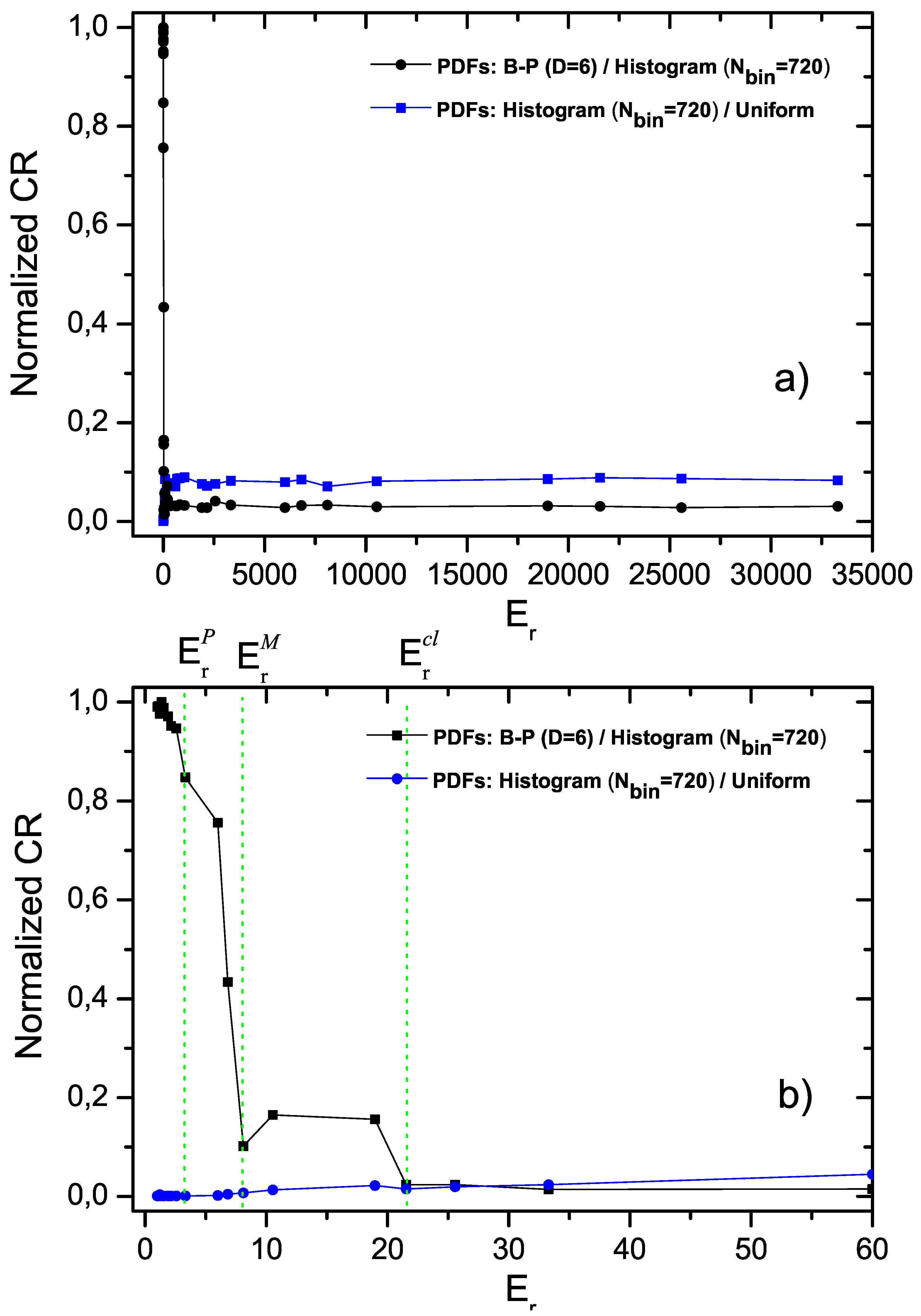
Figure 4.
Normalized Cressie–Read divergence (). I(B-P,histogram,1) and I(histogram,uniform,1) are plotted vs. .
Figure 4.
Normalized Cressie–Read divergence (). I(B-P,histogram,1) and I(histogram,uniform,1) are plotted vs. .
The CR results indicate that the performance of BP is so good that it makes consideration of the histogram PDF irrelevant. Notice that the horizontal coordinate in our graphs is, essentially, an effective Planck constant. At we have the actual Planck value. It vanishes as tends to infinity. We have a signal that represents the system’s state at a given . Sampling that signal we extracted several PDFs. One way of doing this is via histograms. Another way is using the B-P approach. What is suggested by the CR-divergence method is that the histogram-PDF does not provide any information about the physics at hand. This occurs because a uniform PDF contains as much information about the physics as the histogram one!
It seems important to emphasize the following point. Periodicity in the quantal zone is seen in this work to be quite different from that of the logistic map, as indicated by the behavior of the CR-divergence measure. In the logistic case we are concerned with just states, while in the physical example there exists an infinite number of periodic states for which causality turns out to be an important factor, because BP-values are significantly larger than the histogram values (the black lines touches the unity value!).
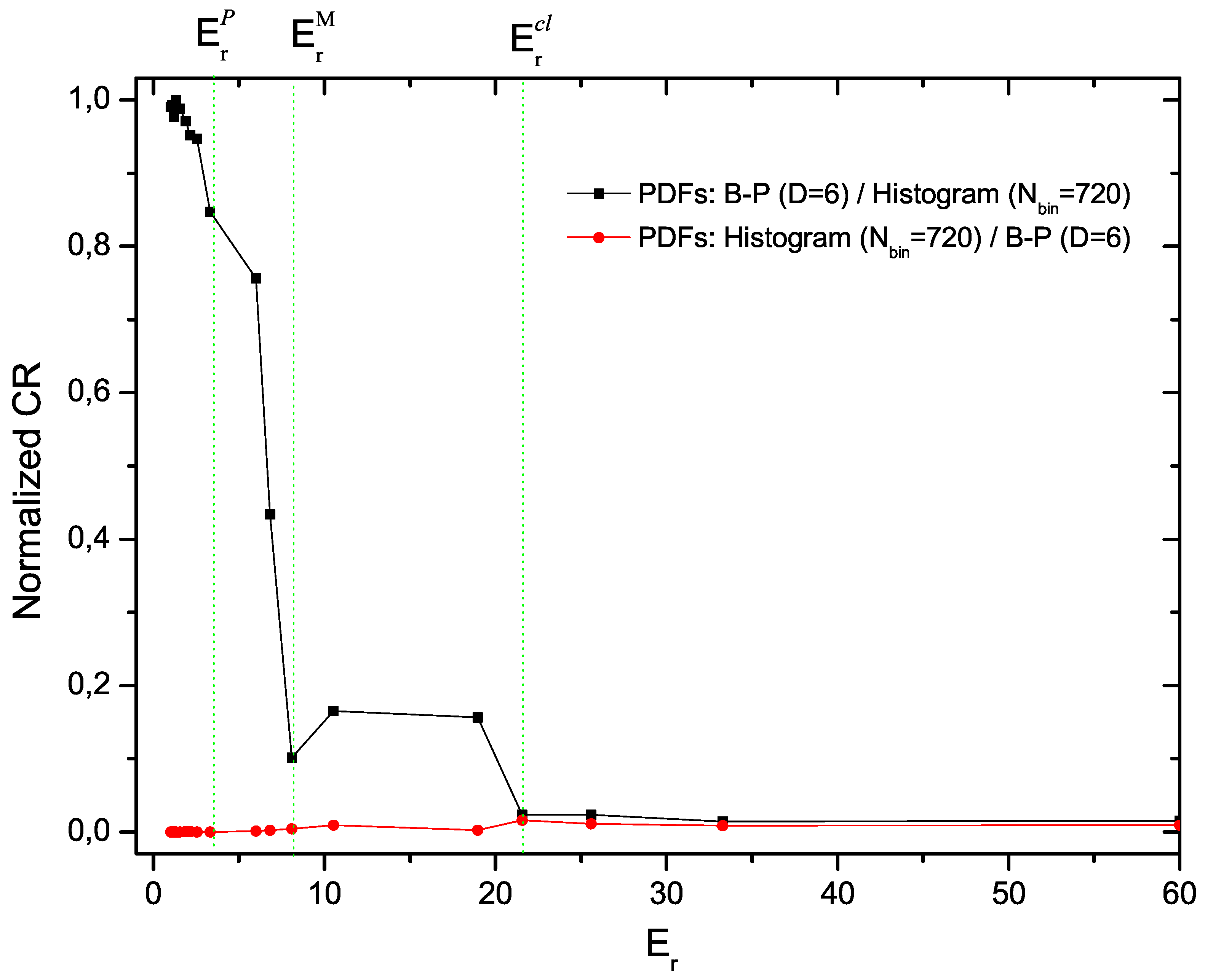
Finally, in
Figure 5 we compare the CR(BP-Histogram), in black, to the CR(Histogram - BP), in red. This comparison indicates that the histogram approach does not add any information to that provided by the BP-PDF.
Figure 5.
Normalized Cressie–Read divergence (). I(B-P,histogram,1) and I(histogram,B-P,1) are plotted vs. .
Figure 5.
Normalized Cressie–Read divergence (). I(B-P,histogram,1) and I(histogram,B-P,1) are plotted vs. .
6. Conclusions
The study and characterization of time series, by recourse to conventional parametric statistical theory tools, assumes that the underlying probability distribution function (PDF) is given. However, for extracting an unknown PDF from the data, a superior nonparametric procedure does not exist. Our present work involves the use of Bandt and Pompe’s methodology for the evaluation of the PDF associated with scalar time series data, using a symbolization technique. The symbolic data are created by ranking the values of the series and defined by reordering the embedded data in ascending order. This yields a phase space reconstruction with embedding dimension (pattern length) D and time lag τ. In this way it is possible to quantify the diversity of the ordering symbols (patterns) derived from a scalar time series, using Bandt–Pompe PDF. It is important to note that the appropriate symbol sequence arises naturally from the time series without any model-based assumptions.
We have employed the CR-divergence measures in order to obtain a definite, quantitative assessment of the superior performance of the BP-approach.
To this end, we have compared the PB approach, via CR-divergence measures, with two other PDFs obtained in different fashion, with reference to the Logistic Map and to a well-known physical problem. We have confirmed the BP-superiority relative to their counterparts and we have also gained some insights concerning details of the physical problem.
Previous papers have examined the relative merits of the histogram
vs. the BP approach (for instance, see the excellent review [
5] and the references therein). However, these approaches rely on visual inspection of the concomitant curves so as to compare signals with their PDF-representatives (for instance, see [
24]). Our work adds an objective assessment, via CR-divergences, that dominates visualization.


