Optimization of MIMO Systems Capacity Using Large Random Matrix Methods

Abstract

This paper provides a comprehensive introduction of large random matrix methods for input covariance matrix optimization of mutual information of MIMO systems. It is first recalled informally how large system approximations of mutual information can be derived. Then, the optimization of the approximations is discussed, and important methodological points that are not necessarily covered by the existing literature are addressed, including the strict concavity of the approximation, the structure of the argument of its maximum, the accuracy of the large system approach with regard to the number of antennas, or the justification of iterative water-filling optimization algorithms. While the existing papers have developed methods adapted to a specific model, this contribution tries to provide a unified view of the large system approximation approach.

1. Introduction

It is now recognized that multiple-input multiple-output (MIMO) systems have the potential to increase the capacity of wireless digital communication systems. If t and r denote the number of transmit and receive antennas, the channel capacity gain can be in fact of the order of $min(t,r)$ under certain (often rather unrealistic) assumptions [1]. Although the use of MIMO systems begins to be normalized, a number of related theoretical issues are still to be solved. This paper addresses the design of input covariance matrices chosen in order to maximize the (Gaussian) mutual information of the system.

This problem was extensively addressed in the past under various assumptions on the channel state information. In this paper, we assume that the channel is known at the receiver side, but that only its probability distribution, which is assumed complex Gaussian, is available at the transmitter side, a context recognized to be realistic in wireless communications, as the channels encountered are mostly fast fading whereas their statistics are slow fading. In this context of fast fading channels, we need to consider the expectation of the mutual information w.r.t. the channel probability distribution instead of the mutual information itself. The optimization of this average mutual information is of course more difficult than the optimization of the mutual information itself, because the analytical expressions of the cost function and of its first- and second-order derivatives are extremely complicated. The optimal input covariance matrix thus cannot be expressed in closed form, and one has to resort to descent algorithms in which the gradient and the Hessian of the cost function have to be evaluated using computationally intensive Monte-Carlo simulations (see e.g., [2] in the context of Rician channels). We note that for certain channel distributions (Rayleigh bi-correlated and uncorrelated Rician channels), the singular vectors of the optimal precoder have closed form expressions, which, of course, simplifies the optimization algorithms (see e.g., [3,4,5]).

Recently, it was proposed to use large random matrix tools to approximate the average mutual information by a large system approximation, and to optimize the approximation versus the input covariance matrix. This optimization problem is easier because the approximation can be very often nearly expressed in closed form so that its maximization does not need Monte-Carlo simulations. Large system approximations of average mutual information were derived in the past using the replica method (see e.g., [6] for bi-correlated MIMO Rayleigh channels, [7] for frequency selective Rayleigh channels, [8] for bi-correlated MIMO Ricean channels, [9] for jointly correlated Rician channel) or rigorous random matrix methods ( [10] for bi-correlated MIMO Rayleigh channels, [11] for bi-correlated MIMO Ricean channels, [12] for frequency selective Rayleigh channels, [13] for multiple access Rayleigh MIMO channels). Optimization algorithms of the large system approximation were first proposed in [14] in the context of bi-correlated MIMO Rayleigh channels. In [11,12] the authors addressed in more details the Rician bi-correlated channels and the frequency selective Rayleigh channels respectively, while [15] considered the Rician channel with interference. In [9] the authors considered the case of jointly correlated Rician channel. Finally, in the context of multiple access Rayleigh MIMO channels, the authors in [13] studied the multiple users input covariance matrices optimization of the related large system approximation. In [16] the authors generalized this analysis in the context of the multiple access jointly correlated Rician MIMO channels. Interestingly, the mutual information provided by the optimization of the approximation appears numerically to be quite close from the true optimum mutual information, even for realistic values of r and t. These observations were confirmed by the theoretical results of [11,12], which showed that the relative error is a $\mathcal{O}\left(\frac{1}{t^2}\right)$ term.

In this paper, we give a comprehensive introduction to the optimization of large system approximations of average mutual information of MIMO channels. We note that the main results of this paper were already presented in [11,12]. However, the focus of [11,12] is on the detailed derivation of the large system approximations, while the present paper concentrates on their optimization. In particular, we emphasize on methodological issues that are often partially—if at all—addressed. Another benefit of this paper is to provide, as much as possible, a unified view of the optimization of the large system approximation in the context of various kinds of MIMO channel, whereas the above referenced papers develop tools that seem specific to each particular model. Generally speaking, the writing style of this paper is rather informal, and hopefully easier to understand. The interested reader may refer to [11,12] for a rigorous presentation.

2. General Principles

2.1. Optimization of the Average Mutual Information

We consider a flat fading MIMO system equipped with t transmit antennas and r receive antennas. In this context, the received observation at time n is a r-variate signal $\mathbf{y}(n)$ given by:

$$\mathbf{y}(n)=\mathbf{H}\mathbf{x}(n)+\mathbf{v}(n)$$

(1)

where $\mathbf{x}(n)$ represents the t-dimensional signal sent at time n at the transmitter side, and where $\mathbf{H}$ is the $r\times t$ channel matrix. ${(\mathbf{v}(n))}_{n\in \mathbb{Z}}$ is a complex white Gaussian noise such that $\mathbb{E}(\mathbf{v}(n)\mathbf{v}{(n)}^H)={\sigma }^2{\mathbf{I}}_r$.

Channel matrix $\mathbf{H}$ is assumed to be a complex Gaussian random matrix (Matrix $\mathbf{H}$ is said complex Gaussian if the $rt$-dimensional vector $\mathbf{h}=\mathrm{vec}(\mathbf{H})$ is complex Gaussian, i.e., the probability distribution of ${(\mathrm{Re}{(\mathbf{h})}^T,\mathrm{Im}{(\mathbf{h})}^T)}^T$ is Gaussian and if $\mathbb{E}\left[(\mathbf{h}-\mathbb{E}(\mathbf{h})){(\mathbf{h}-\mathbb{E}(\mathbf{h}))}^T\right]=0$) whose current value is known at the receiver side and whose probability distribution is known at the transmitter side. If $\mathbf{Q}$ denotes the covariance matrix of $\mathbf{x}(n)$ normalized in such a way that $\frac{1}{t}\mathrm{Tr}(\mathbf{Q})=1$, the (Gaussian) average mutual information of model (1) is given by [1]:

$$I(\mathbf{Q})={\mathbb{E}}_{\mathbf{H}}log\det \left[{\mathbf{I}}_r+\frac{\mathbf{H}\mathbf{Q}{\mathbf{H}}^H}{{\sigma }^2}\right]$$

(2)

where ${\mathbb{E}}_{\mathbf{H}}$ represents the mathematical expectation operator w.r.t. the distribution of matrix $\mathbf{H}$.

In the following, we denote by $\mathcal{C}$ the cone of all non-negative (positive semi-definite) matrices $\mathbf{Q}$, and by ${\mathcal{C}}_1$ the set of all matrices $\mathbf{Q}\in \mathcal{C}$ for which $\frac{1}{t}\mathrm{Tr}(\mathbf{Q})=1$. The ergodic capacity of the channel model (1) is defined as the maximum of $I(\mathbf{Q})$ over the set ${\mathcal{C}}_1$, and is known to represent the maximum rate that can be transmitted reliably when $\mathbf{H}$ is known at the receiver and when its probability distribution is known at the transmitter side. In particular, using as input covariance matrix the argument of the maximum of $I(\mathbf{Q})$ allows to transmit reliably at the largest possible rate. This explains why the maximization of $I(\mathbf{Q})$ over the set ${\mathcal{C}}_1$ is important.

Function $\mathbf{Q}\to I(\mathbf{Q})$ is concave, and under some additional assumptions, strictly concave on the convex set ${\mathcal{C}}_1$. Therefore ([17]), the maximization of $I(\mathbf{Q})$ over ${\mathcal{C}}_1$ has a unique argument, which is denoted ${\mathbf{Q}}_{*}$ in the following. In general, ${\mathbf{Q}}_{*}$ has no closed form expression. Therefore, its evaluation needs the use of descent algorithms which, due to the concavity of I and the convexity of ${\mathcal{C}}_1$, are convergent. In order to implement such algorithms, it is necessary to be able to evaluate I and its first and second derivatives at each point. As the analytical expressions of these functions are in general extremely complicated, the simplest solution consists in using Monte-Carlo evaluations. This, of course, leads to computationally intensive algorithms.

2.2. Large System Approximation of $I(\mathbf{Q})$

2.2.1. The Case $\mathbf{Q}=\mathbf{I}$

In this paragraph, we first introduce informally how it is possible to derive a large system approximation of the mutual information $I(\mathbf{I})$ corresponding to the case where the covariance matrix of the transmitted signal is $\mathbf{Q}=\mathbf{I}$. In order to simplify the notations, we denote $I(\mathbf{I})$ by I.

Background on the behaviour of the eigenvalue distribution of $\mathbf{H}{\mathbf{H}}^H$ Let ${\mathbf{H}}_{r,t}$ be a $r\times t$ complex Gaussian random matrix representing the channel matrix of a MIMO system (we indicate that $\mathbf{H}$ is a $r\times t$ matrix by denoting $\mathbf{H}$ by ${\mathbf{H}}_{r,t}$), and consider its associated Gram matrix defined by ${\mathbf{H}}_{r,t}{\mathbf{H}}_{r,t}^H$. Under certain assumptions on the probability distribution of ${\mathbf{H}}_{r,t}$ (see the examples below), it appears that the empirical eigenvalue distribution ${\widehat{\mu }}_{r,t}$ of ${\mathbf{H}}_{r,t}{\mathbf{H}}_{r,t}^H$ defined as $\frac{1}{r}{\sum }_{i=1}^r\delta \left(\lambda -{\lambda }_i({\mathbf{H}}_{r,t}{\mathbf{H}}_{r,t}^H)\right)$ tends to have a deterministic behaviour when the dimensions r and t converge to $+\infty$ in such a way that $\frac{t}{r}\to c$, where $0<c<+\infty$. In order to shorten the notations, $t\to +\infty$ stands in the following for r and t converge to $+\infty$ in such a way that $\frac{t}{r}\to c$. This is equivalent to saying that it exists deterministic probability measures ${\mu }_{r,t}$ (which depend on the dimensions r and t) for which

$$\frac{1}{r}\sum _{i=1}^r\varphi \left({\lambda }_i({\mathbf{H}}_{r,t}{\mathbf{H}}_{r,t}^H)\right)-\int \varphi (\lambda )d{\mu }_{r,t}(\lambda )\to 0$$

(3)

almost surely when $t\to +\infty$ for each well chosen test function φ. Sometimes, the measures ${\mu }_{r,t}$ also converge towards a probability distribution ${\mu }_{*}$, which does not depend on the values of $(r,t)$ but only on $c=lim\frac{t}{r}$. In this case, the eigenvalue distribution converges towards ${\mu }_{*}$, which is called the limit eigenvalue distribution ${\mathbf{H}}_{r,t}{\mathbf{H}}_{r,t}^H$. In order to illustrate the above phenomenon, we consider the simplest situation in which the entries of ${\mathbf{H}}_{r,t}$ are independent identically distributed (i.i.d.) zero mean random variables of variance $\frac{1}{t}$, and where $c\le 1$. In this case, the measure ${\mu }_{r,t}$ is absolutely continuous, and its density $p_{r,t}(\lambda )$ is given by:

$$\begin{array}{ccc}\hfill p_{r,t}(\lambda )& =& \frac{r}{2\pi \lambda }\sqrt{[{(1+\sqrt{1/r})}^2-\lambda ][\lambda -{(1-\sqrt{1/r})}^2]}\hfill \\ & & if\lambda \in [{(1-\sqrt{1/r})}^2,{(1+\sqrt{1/r})}^2]\hfill \\ & =& 0\mathrm{otherwise}\hfill \end{array}$$

The corresponding distribution is called the Marčenko–Pastur distribution, and was introduced for the first time in [18].

In order to simplify the notations, we no longer mention the dimensions r and t in the following, and denote ${\mathbf{H}}_{r,t},{\widehat{\mu }}_{r,t},{\mu }_{r,t}$ by $\mathbf{H},\widehat{\mu },\mu$ respectively. In order to establish that $\widehat{\mu }$ has a deterministic behaviour when $t\to +\infty$, it is well known that it is sufficient to establish that (3) holds for $\varphi (\lambda )=\frac{1}{\lambda +{\sigma }^2}$ for each ${\sigma }^2>0$ (see e.g., [19,20]). In order to reformulate (3) for $\varphi (\lambda )=\frac{1}{\lambda +{\sigma }^2}$, we introduce the Stieltjes transform $s_{\nu }$ of a positive measure ν carried by ${\mathbb{R}}^{+}$, which is the function defined for each $z\in \mathbb{C}-{\mathbb{R}}^{-}$ as:

$$s_{\nu }(z)={\int }_{{\mathbb{R}}^{+}}\frac{1}{\lambda +z}d\nu (\lambda )$$

(4)

Equation (3) for $\varphi (\lambda )=\frac{1}{\lambda +{\sigma }^2}$ for each ${\sigma }^2>0$ is thus equivalent to:

$$\underset{t\to +\infty }{lim}\left[s_{\widehat{\mu }}({\sigma }^2)-s_{\mu }({\sigma }^2)\right]=0$$

(5)

for each ${\sigma }^2>0$ because

$$s_{\widehat{\mu }}({\sigma }^2)=\frac{1}{r}\sum _{i=1}^r\frac{1}{{\lambda }_i\left(\mathbf{H}{\mathbf{H}}^H\right)+{\sigma }^2}$$

and

$$s_{\mu }({\sigma }^2)={\int }_{{\mathbb{R}}^{+}}\frac{1}{\lambda +{\sigma }^2}d\mu (\lambda )$$

In order to prove (5), a possible approach is to establish that $s_{\widehat{\mu }}({\sigma }^2)$ has the same asymptotic behaviour as a deterministic quantity which appears to coincide with the value at point ${\sigma }^2$ of the Stieltjes transform of a certain probability measure μ carried by ${\mathbb{R}}^{+}$. For this, it is useful to introduce the resolvent of matrix $\mathbf{H}{\mathbf{H}}^H$ defined as the $r\times r$ matrix valued function $\mathbf{S}$ defined for each ${\sigma }^2>0$ by:

$$\mathbf{S}({\sigma }^2)={\left(\mathbf{H}{\mathbf{H}}^H+{\sigma }^2{\mathbf{I}}_r\right)}^{-1}$$

(6)

It is important to notice that

$$s_{\widehat{\mu }}({\sigma }^2)=\frac{1}{r}\mathrm{Tr}\mathbf{S}({\sigma }^2)$$

(7)

Under suitable hypotheses on $\mathbf{H}$, the random entries of $\mathbf{S}({\sigma }^2)$ turn out to have the same behaviour as the entries of a deterministic $r\times r$ matrix $\mathbf{T}({\sigma }^2)$, which, in particular, implies that

$$\frac{1}{r}\mathrm{Tr}\mathbf{S}({\sigma }^2)-\frac{1}{r}\mathrm{Tr}\mathbf{T}({\sigma }^2)\to 0$$

The entries of matrix $\mathbf{T}({\sigma }^2)$ can be expressed in closed form in terms of the (unique) positive solutions ${({\delta }_j({\sigma }^2))}_{j=1,\dots ,n},{({\tilde{\delta }}_i({\sigma }^2))}_{i=1,\dots ,m}$ of a nonlinear system of $n+m$ equations depending on $r,t$, ${\sigma }^2$, and the statistical properties of $\mathbf{H}$. This nonlinear system of equations is called in [21] the canonical equations associated to the random matrix model $\mathbf{H}$. The number of unknowns $m+n$ depends on $r,t$ and the statistics of $\mathbf{H}$. Then, it is shown that function ${\sigma }^2\to \frac{1}{r}\mathrm{Tr}\mathbf{T}({\sigma }^2)$ coincides with the Stieltjes transform of a certain probability measure μ, which, in turn, establishes that (5) holds for each ${\sigma }^2$. It is also useful to notice that the entries of matrix $\tilde{\mathbf{S}}({\sigma }^2)$ defined as

$$\tilde{\mathbf{S}}({\sigma }^2)={\left({\mathbf{H}}^H\mathbf{H}+{\sigma }^2{\mathbf{I}}_t\right)}^{-1}$$

(8)

have the same behaviour as the entries of a $t\times t$ deterministic matrix $\tilde{\mathbf{T}}({\sigma }^2)$. These entries can be evaluated in terms of the solutions of the above-mentioned canonical equations.

We also mention that it is often possible to evaluate the accuracy of the approximations. In the context of a number of complex Gaussian random matrix models, it holds that

$$\begin{array}{ccc}\hfill \mathbb{E}{\left|\frac{1}{r}\mathrm{Tr}\mathbf{S}({\sigma }^2)-\mathbb{E}\frac{1}{r}\mathrm{Tr}\mathbf{S}({\sigma }^2)\right|}^2& =& \mathcal{O}\left(\frac{1}{t^2}\right)\hfill \end{array}$$

(9)

$$\begin{array}{ccc}\hfill \mathbb{E}\left[\frac{1}{r}\mathrm{Tr}\mathbf{S}({\sigma }^2)\right]-\frac{1}{r}\mathrm{Tr}\mathbf{T}({\sigma }^2)& =& \mathcal{O}\left(\frac{1}{t^2}\right)\hfill \end{array}$$

(10)

Large system approximation of I We finally consider the problem of approximating $I=\mathbb{E}\left(log\det ({\mathbf{I}}_r+\frac{1}{{\sigma }^2}\mathbf{H}{\mathbf{H}}^H)\right)$. We first note that

$$\frac{1}{r}log\det ({\mathbf{I}}_r+\frac{1}{{\sigma }^2}\mathbf{H}{\mathbf{H}}^H)=\frac{1}{r}\sum _{i=1}^{r}log\left(1+{\lambda }_i(\mathbf{H}{\mathbf{H}}^H)/{\sigma }^2\right)$$

and thus coincides with a functional of the eigenvalues of $\mathbf{H}{\mathbf{H}}^H$. It can therefore be approximated by a deterministic term that can very often be expressed in an explicit way. In order to explain this, we use the following well-known identity:

$$\frac{1}{r}log\det \left(\mathbf{I}+\frac{1}{{\sigma }^2}\mathbf{H}{\mathbf{H}}^H\right)={\int }_{{\sigma }^2}^{+\infty }\left(\frac{1}{{\omega }^2}-\frac{1}{r}\mathrm{Tr}\mathbf{S}({\omega }^2)\right)d{\omega }^2$$

(11)

As $\frac{1}{r}\mathrm{Tr}\mathbf{S}({\omega }^2)$ can be approximated by $\frac{1}{r}\mathrm{Tr}\mathbf{T}({\omega }^2)$, it can be shown that

$$\frac{1}{r}log\det \left(\mathbf{I}+\frac{1}{{\sigma }^2}\mathbf{H}{\mathbf{H}}^H\right)-{\int }_{{\sigma }^2}^{+\infty }\left(\frac{1}{{\omega }^2}-\frac{1}{r}\mathrm{Tr}\mathbf{T}({\omega }^2)\right)d{\omega }^2\to 0$$

(12)

But, in the context of the various usual MIMO models, it turns out that

$${\int }_{{\sigma }^2}^{+\infty }\left(\frac{1}{{\omega }^2}-\frac{1}{r}\mathrm{Tr}\mathbf{T}({\omega }^2)\right)d{\omega }^2=\frac{1}{r}\left[log\det {\left({\sigma }^2\mathbf{T}({\sigma }^2)\right)}^{-1}+log\det {\left({\sigma }^2\tilde{\mathbf{T}}({\sigma }^2)\right)}^{-1}-g({\sigma }^2,\delta ({\sigma }^2),\tilde{\delta }({\sigma }^2))\right]$$

(13)

where $\delta ({\sigma }^2)={({\delta }_1({\sigma }^2),\dots ,{\delta }_n({\sigma }^2))}^T$ and $\tilde{\delta }({\sigma }^2)={({\tilde{\delta }}_1({\sigma }^2),\dots ,{\tilde{\delta }}_m({\sigma }^2))}^T$ represent the solutions of the nonlinear system of $m+n$ equations governing the entries of $\mathbf{T}({\sigma }^2)$ and where g is a well chosen function that is expressed in closed form. Taking the mathematical expectation of (12), and using that the error between $\mathbb{E}\left(\frac{1}{r}\mathrm{Tr}\mathbf{S}({\omega }^2)\right)$ and $\frac{1}{r}\mathrm{Tr}\mathbf{T}({\omega }^2)$ is a $\mathcal{O}\left(\frac{1}{t^2}\right)$ term for each ${\omega }^2$ (see Equation (10)), it can be shown that

$$\begin{array}{cc}\hfill I/r& =\mathbb{E}\left[\frac{1}{r}log\det \left(\mathbf{I}+\frac{1}{{\sigma }^2}\mathbf{H}{\mathbf{H}}^H\right)\right]\hfill \\ & =\frac{1}{r}\left[log\det {\left({\sigma }^2\mathbf{T}({\sigma }^2)\right)}^{-1}+log\det {\left({\sigma }^2\tilde{\mathbf{T}}({\sigma }^2)\right)}^{-1}-g({\sigma }^2,\delta ({\sigma }^2),\tilde{\delta }({\sigma }^2))\right]+\mathcal{O}\left(\frac{1}{t^2}\right)\hfill \end{array}$$

or equivalently

$$I=\overline{I}+\mathcal{O}\left(\frac{1}{t}\right)$$

(14)

where the large system approximation $\overline{I}$ of I is defined by:

$$\overline{I}=log\det {\left({\sigma }^2\mathbf{T}({\sigma }^2)\right)}^{-1}+log\det {\left({\sigma }^2\tilde{\mathbf{T}}({\sigma }^2)\right)}^{-1}-g({\sigma }^2,\delta ({\sigma }^2),\tilde{\delta }({\sigma }^2))$$

As I and $\overline{I}$ scale linearly with t when t increases, Ref (14) implies that the relative error between I and its large system approximation is a $\mathcal{O}\left(\frac{1}{t^2}\right)$ term, and thus decreases rather fast towards 0 when t increases. This explains partially why large system approximation of mutual information are very accurate even for moderate number of transmit and receive antennas.

Examples 

In order to illustrate these results, we provide the expressions of $\mathbf{T},\tilde{\mathbf{T}}$ and $\overline{I}$ in the context of useful random matrix models. We first consider the case where $\mathbf{H}$ can be written as:

$$\mathbf{H}=\frac{1}{\sqrt{t}}{\mathbf{C}}^{1/2}\mathbf{X}{\tilde{\mathbf{C}}}^{1/2}$$

(15)

where the entries of $\mathbf{X}$ are complex Gaussian i.i.d. random variables with zero mean and variance 1 and where $\mathbf{C}$ and $\tilde{\mathbf{C}}$ are $r\times r$ and $t\times t$ deterministic positive matrices such that

$$\underset{r}{sup}\parallel \mathbf{C}\parallel <+\infty ,\underset{t}{sup}\parallel \tilde{\mathbf{C}}\parallel <+\infty$$

(16)

Then, it can be shown that the nonlinear system of equations:

$$\begin{array}{ccc}\hfill \kappa & =& \frac{1}{t}\mathrm{Tr}\mathbf{C}{\left[{\sigma }^2({\mathbf{I}}_r+\tilde{\kappa }\mathbf{C})\right]}^{-1}\hfill \end{array}$$

(17)

$$\begin{array}{ccc}\hfill \tilde{\kappa }& =& \frac{1}{t}\mathrm{Tr}\tilde{\mathbf{C}}{\left[{\sigma }^2({\mathbf{I}}_t+\kappa \tilde{\mathbf{C}})\right]}^{-1}\hfill \end{array}$$

(18)

has a unique pair of positive solutions denoted $(\delta ({\sigma }^2),\tilde{\delta }({\sigma }^2))$. Matrices $\mathbf{T}({\sigma }^2)$ and $\tilde{\mathbf{T}}({\sigma }^2)$ introduced above are given by:

$$\begin{array}{ccc}\hfill \mathbf{T}({\sigma }^2)& =& {\left[{\sigma }^2({\mathbf{I}}_r+\tilde{\delta }({\sigma }^2)\mathbf{C})\right]}^{-1}\hfill \end{array}$$

(19)

$$\begin{array}{ccc}\hfill \tilde{\mathbf{T}}({\sigma }^2)& =& {\left[{\sigma }^2({\mathbf{I}}_t+\delta ({\sigma }^2)\tilde{\mathbf{C}})\right]}^{-1}\hfill \end{array}$$

(20)

The two canonical equations defining $(\delta ({\sigma }^2),\tilde{\delta }({\sigma }^2))$ can therefore be written as:

$$\begin{array}{ccc}\hfill \delta ({\sigma }^2)& =& \frac{1}{t}\mathrm{Tr}\mathbf{C}\mathbf{T}({\sigma }^2)\hfill \end{array}$$

(21)

$$\begin{array}{ccc}\hfill \tilde{\delta }({\sigma }^2)& =& \frac{1}{t}\mathrm{Tr}\tilde{\mathbf{C}}\tilde{\mathbf{T}}({\sigma }^2)\hfill \end{array}$$

(22)

The corresponding large system approximation $\overline{I}$ of I is given by:

$$\overline{I}=log\det \left(\mathbf{I}+\tilde{\delta }({\sigma }^2)\mathbf{C}\right)+log\det \left(\mathbf{I}+\delta ({\sigma }^2)\tilde{\mathbf{C}}\right)-t{\sigma }^2\delta ({\sigma }^2)\tilde{\delta }({\sigma }^2)$$

(23)

so that function g defined by Equation (13) is given by $g({\sigma }^2,\delta ,\tilde{\delta })=t{\sigma }^2\delta \tilde{\delta }$. It is useful to justify the above expression of $\overline{I}$ because the proof below extends in the context of other models. For this, it is necessary to establish that Equation (13) holds for the above function g. It can be shown that the right-hand side of (23) converges towards 0 when ${\sigma }^2\to +\infty$. Therefore, it remains to check that the derivative w.r.t. ${\sigma }^2$ of the right-hand side of (23) coincides with $-r\left(\frac{1}{{\sigma }^2}-\frac{1}{r}\mathrm{Tr}\mathbf{T}({\sigma }^2)\right)$. We introduce the following function $V({\sigma }^2,\kappa ,\tilde{\kappa })$ of three variables:

$$V({\sigma }^2,\kappa ,\tilde{\kappa })=log\det \left(\mathbf{I}+\tilde{\kappa }\mathbf{C}\right)+log\det \left(\mathbf{I}+\kappa \tilde{\mathbf{C}}\right)-t{\sigma }^2\kappa \tilde{\kappa }$$

(24)

which is obtained by replacing $(\delta ({\sigma }^2),\tilde{\delta }({\sigma }^2))$ with the fixed parameters $(\kappa ,\tilde{\kappa })$ into the expression of the right-hand side of (23). A very important property of function V is:

$$\begin{array}{ccc}\hfill {\left(\frac{\partial V}{\partial \kappa }\right)}_{\kappa =\delta ({\sigma }^2),\tilde{\kappa }=\tilde{\delta }({\sigma }^2)}& =& 0\hfill \end{array}$$

(25)

$$\begin{array}{ccc}\hfill {\left(\frac{\partial V}{\partial \tilde{\kappa }}\right)}_{\kappa =\delta ({\sigma }^2),\tilde{\kappa }=\tilde{\delta }({\sigma }^2)}& =& 0\hfill \end{array}$$

(26)

In fact, it is straightforward that

$${\left(\frac{\partial V}{\partial \kappa }\right)}_{\kappa =\delta ({\sigma }^2),\tilde{\kappa }=\tilde{\delta }({\sigma }^2)}=\mathrm{Tr}\left(\tilde{\mathbf{C}}{\left[\mathbf{I}+\delta ({\sigma }^2)\tilde{\mathbf{C}}\right]}^{-1}\right)-t{\sigma }^2\tilde{\delta }({\sigma }^2)$$

and vanishes because $\tilde{\delta }({\sigma }^2)$ satisfies the canonical Equation (22). We obtain similarly that (26) holds because $\delta ({\sigma }^2)$ is the solution of the canonical Equation (21). In sum, it appears that (25, 26) are equivalent to the canonical Equations 19 and 20.

The derivative w.r.t. ${\sigma }^2$ of the right-hand side of (23) is given by:

$${\left(\frac{\partial V}{\partial \kappa }\right)}_{\kappa =\delta ({\sigma }^2),\tilde{\kappa }=\tilde{\delta }({\sigma }^2)}\frac{d\delta }{d{\sigma }^2}+{\left(\frac{\partial V}{\partial \tilde{\kappa }}\right)}_{\kappa =\delta ({\sigma }^2),\tilde{\kappa }=\tilde{\delta }({\sigma }^2)}\frac{d\tilde{\delta }}{d{\sigma }^2}-t\delta ({\sigma }^2)\tilde{\delta }({\sigma }^2)$$

and thus coincides with $-t\delta ({\sigma }^2)\tilde{\delta }({\sigma }^2)$ by (25, 26). Using (21, 22) as well as the expressions (19, 20) of $\mathbf{T}({\sigma }^2)$ and $\tilde{\mathbf{T}}({\sigma }^2)$, this is easily seen to be equal to $-r\left(\frac{1}{{\sigma }^2}-\frac{1}{r}\mathrm{Tr}\mathbf{T}({\sigma }^2)\right)$; indeed,

$$\frac{r}{{\sigma }^2}-\mathrm{Tr}\mathbf{T}({\sigma }^2)=\mathrm{Tr}\left[\left({\left({\sigma }^2\mathbf{T}({\sigma }^2)\right)}^{-1}-{\mathbf{I}}_r\right)\mathbf{T}\right]=\mathrm{Tr}\left[\left(({\mathbf{I}}_r+\tilde{\delta }({\sigma }^2)\mathbf{C})-{\mathbf{I}}_r\right)\mathbf{T}\right]=t\delta ({\sigma }^2)\tilde{\delta }({\sigma }^2)$$

Hence, both sides of (13) have the same derivative w.r.t. ${\sigma }^2$. Moreover, both sides converge towards 0 when ${\sigma }^2\to +\infty$, thus Equation (13) is verified for $g({\sigma }^2,\delta ,\tilde{\delta })=t{\sigma }^2\delta \tilde{\delta }$. This, together with (12), establishes that (23) holds.

We now consider the case where channel $\mathbf{H}$ is given as:

$$\mathbf{H}=\sum _{l=1}^L\frac{1}{\sqrt{t}}{\mathbf{C}}_l^{1/2}{\mathbf{X}}_l{\tilde{\mathbf{C}}}_l^{1/2}$$

(27)

where matrices ${({\mathbf{X}}_l)}_{l=1,\dots ,L}$ are mutually independent complex Gaussian random matrices with i.i.d. entries of mean 0 and variance 1 and where ${\mathbf{C}}_l$ and ${\tilde{\mathbf{C}}}_l$ are $r\times r$ and $t\times t$ deterministic positive matrices such that

$$\underset{r}{sup}\parallel {\mathbf{C}}_l\parallel <+\infty ,\underset{t}{sup}\parallel {\tilde{\mathbf{C}}}_l\parallel <+\infty$$

(28)

for $l=1,\dots ,L$. It is important to notice that the parameter L is independent of r and t, and thus does not scale with the number of antennas. As shown in [7,12], model (27) is useful in the context of multipath channels with independent paths. Matrices $\mathbf{T}$ and $\tilde{\mathbf{T}}$ are given by:

$$\begin{array}{ccc}\hfill \mathbf{T}({\sigma }^2)& =& {\left[{\sigma }^2({\mathbf{I}}_r+\sum _{l=1}^L{\tilde{\delta }}_l({\sigma }^2){\mathbf{C}}_l)\right]}^{-1}\hfill \end{array}$$

(29)

$$\begin{array}{ccc}\hfill \tilde{\mathbf{T}}({\sigma }^2)& =& {\left[{\sigma }^2({\mathbf{I}}_t+\sum _{l=1}^L{\delta }_l({\sigma }^2){\tilde{\mathbf{C}}}_l)\right]}^{-1}\hfill \end{array}$$

(30)

where the ${({\delta }_l({\sigma }^2),{\tilde{\delta }}_l({\sigma }^2))}_{l=1,\dots ,L}$ are the unique positive solutions of the system of $2L$ equations:

$$\begin{array}{ccc}\hfill {\delta }_l({\sigma }^2)& =& \frac{1}{t}\mathrm{Tr}{\mathbf{C}}_l\mathbf{T}({\sigma }^2)\hfill \end{array}$$

(31)

$$\begin{array}{ccc}\hfill {\tilde{\delta }}_l({\sigma }^2)& =& \frac{1}{t}\mathrm{Tr}{\tilde{\mathbf{C}}}_l\tilde{\mathbf{T}}({\sigma }^2)\hfill \end{array}$$

(32)

for $l=1,\dots ,L$. The large system approximation of I is this time given by [7,12]:

$$\overline{I}=log\det \left(\mathbf{I}+\sum _{l=1}^L{\tilde{\delta }}_l({\sigma }^2){\mathbf{C}}_l\right)+log\det \left(\mathbf{I}+\sum _{l=1}^L{\delta }_l({\sigma }^2){\tilde{\mathbf{C}}}_l\right)-t{\sigma }^2\sum _{l=1}^L{\delta }_l({\sigma }^2){\tilde{\delta }}_l({\sigma }^2)$$

(33)

and thus corresponds to Equation (14) when $g({\sigma }^2,\delta ,\tilde{\delta })=t{\sigma }^2{\delta }^T\tilde{\delta }=t{\sigma }^2{\sum }_{l=1}^L{\delta }_l{\tilde{\delta }}_l$. (33) is proved in the same way as (23) by introducing the function of $2L+1$ variables $V({\sigma }^2,\kappa ,\tilde{\kappa })$ obtained by replacing into the right-hand side of (33) functions $\delta ({\sigma }^2)$, $\tilde{\delta }({\sigma }^2)$ by fixed vectors κ and $\tilde{\kappa }$, and by observing that the canonical Equations (31, 32) are equivalent to:

$$\begin{array}{ccc}\hfill {\left(\frac{\partial V}{\partial {\kappa }_l}\right)}_{\kappa =\delta ({\sigma }^2),\tilde{\kappa }=\tilde{\delta }({\sigma }^2)}& =& 0\hfill \end{array}$$

(34)

$$\begin{array}{ccc}\hfill {\left({\frac{\partial V}{\partial \tilde{\kappa }}}_l\right)}_{\kappa =\delta ({\sigma }^2),\tilde{\kappa }=\tilde{\delta }({\sigma }^2)}& =& 0\hfill \end{array}$$

(35)

We now consider a third random matrix model modeling bi-correlated Rician channels. We assume that $\mathbf{H}$ can be written as:

$$\mathbf{H}=\mathbf{A}+\frac{1}{\sqrt{t}}{\mathbf{C}}^{1/2}\mathbf{X}{\tilde{\mathbf{C}}}^{1/2}$$

(36)

where the entries of $\mathbf{X}$ are complex Gaussian i.i.d. random variables with zero mean and variance 1 and where $\mathbf{C}$ and $\tilde{\mathbf{C}}$ are $r\times r$ and $t\times t$ deterministic positive matrices such that

$$\underset{r}{sup}\parallel \mathbf{C}\parallel <+\infty ,\underset{t}{sup}\parallel \tilde{\mathbf{C}}\parallel <+\infty$$

(37)

Matrix $\mathbf{A}$ is a deterministic $r\times t$ matrix satisfying:

$$\underset{r,t}{sup}\parallel \mathbf{A}\parallel <+\infty$$

(38)

This time, matrices $\mathbf{T}({\sigma }^2)$ and $\tilde{\mathbf{T}}({\sigma }^2)$ are given by:

$$\begin{array}{ccc}\hfill \mathbf{T}({\sigma }^2)& =& {\left[{\sigma }^2({\mathbf{I}}_r+\tilde{\delta }({\sigma }^2)\mathbf{C})+\mathbf{A}{(\mathbf{I}+\delta ({\sigma }^2)\tilde{\mathbf{C}})}^{-1}{\mathbf{A}}^H\right]}^{-1}\hfill \end{array}$$

(39)

$$\begin{array}{ccc}\hfill \tilde{\mathbf{T}}({\sigma }^2)& =& {\left[{\sigma }^2({\mathbf{I}}_t+\delta ({\sigma }^2)\tilde{\mathbf{C}})+{\mathbf{A}}^H{(\mathbf{I}+\tilde{\delta }({\sigma }^2)\mathbf{C})}^{-1}\mathbf{A}\right]}^{-1}\hfill \end{array}$$

(40)

where $(\delta ({\sigma }^2),\tilde{\delta }({\sigma }^2))$ satisfy the same canonical Equations (21, 22) as in the case of the Rayleigh bi-correlated MIMO channels, i.e.,

$$\begin{array}{ccc}\hfill \delta ({\sigma }^2)& =& \frac{1}{t}\mathrm{Tr}\mathbf{C}\mathbf{T}({\sigma }^2)\hfill \end{array}$$

(41)

$$\begin{array}{ccc}\hfill \tilde{\delta }({\sigma }^2)& =& \frac{1}{t}\mathrm{Tr}\tilde{\mathbf{C}}\tilde{\mathbf{T}}({\sigma }^2)\hfill \end{array}$$

(42)

It can be shown as previously that the corresponding large system approximation $\overline{I}$ of I is now given by [11,22]:

$$\overline{I}=log\det \left(\mathbf{I}+\tilde{\delta }({\sigma }^2)\mathbf{C}\right)+log\det \left(\mathbf{I}+\delta ({\sigma }^2)\tilde{\mathbf{C}}+\frac{1}{{\sigma }^2}{\mathbf{A}}^H{(\mathbf{I}+\tilde{\delta }({\sigma }^2)\mathbf{C})}^{-1}\mathbf{A}\right)-t{\sigma }^2\delta ({\sigma }^2)\tilde{\delta }({\sigma }^2)$$

(43)

and corresponds to Equation (14) when $g({\sigma }^2,\delta ,\tilde{\delta })$ is equal to:

$$g({\sigma }^2,\delta ,\tilde{\delta })=log\det \left(\mathbf{I}+\frac{1}{{\sigma }^2}{(\mathbf{I}+\tilde{\delta }\mathbf{C})}^{-1}\mathbf{A}{(\mathbf{I}+\tilde{\delta }\mathbf{C})}^{-1}{\mathbf{A}}^H\right)+t{\sigma }^2\delta \tilde{\delta }$$

(44)

A slightly more general non-zero mean MIMO model is:

$$\mathbf{H}=\mathbf{A}+\frac{1}{\sqrt{t}}\mathbf{U}\left(\mathbf{D}\circ \mathbf{X}\right){\mathbf{V}}^H$$

(45)

where ∘ represents the Schur–Hadamard product, where $\mathbf{D}$ represents a $r\times t$ matrix such that ${\mathbf{D}}_{i,j}\ge 0$ and ${sup}_{r,t}\parallel \mathbf{D}\parallel <+\infty$, and where $\mathbf{U}$ and $\mathbf{V}$ are deterministic unitary $r\times r$ and $t\times t$ matrices. $\mathbf{A}$ and $\mathbf{X}$ have the same properties as in the context of model (36). This MIMO channel model was introduced in [23], studied in the large system regime in the zero mean case in [10] and in the non-zero mean case in [24] and, using the replica method, more recently in [9,16] in the context of the MIMO multi-access channel. As we are essentially interested by the functionals of the eigenvalues of $\mathbf{H}{\mathbf{H}}^H$, it is possible to assume without restrictions that $\mathbf{U}$ and $\mathbf{V}$ are reduced to ${\mathbf{I}}_r$ and ${\mathbf{I}}_t$ respectively. In this case, matrices $\mathbf{T}$ and $\tilde{\mathbf{T}}$ are given by:

$$\begin{array}{ccc}\hfill \mathbf{T}({\sigma }^2)& =& {\left[{\sigma }^2({\mathbf{I}}_r+\tilde{\Delta }({\sigma }^2))+\mathbf{A}{(\mathbf{I}+\Delta ({\sigma }^2))}^{-1}{\mathbf{A}}^H\right]}^{-1}\hfill \end{array}$$

(46)

$$\begin{array}{ccc}\hfill \tilde{\mathbf{T}}({\sigma }^2)& =& {\left[{\sigma }^2({\mathbf{I}}_t+\Delta ({\sigma }^2))+{\mathbf{A}}^H(\mathbf{I}+\tilde{\Delta }{({\sigma }^2)}^{-1})\mathbf{A}\right]}^{-1}\hfill \end{array}$$

(47)

where $\Delta ({\sigma }^2)=\mathrm{Diag}({\delta }_1({\sigma }^2),\dots ,{\delta }_t({\sigma }^2))$ and $\tilde{\Delta }({\sigma }^2)=\mathrm{Diag}({\tilde{\delta }}_1({\sigma }^2),\dots ,{\tilde{\delta }}_r({\sigma }^2))$ are two diagonal $t\times t$ and $r\times r$ matrices whose elements are the positive solutions of the equations:

$$\begin{array}{ccc}\hfill {\delta }_j({\sigma }^2)& =& \frac{1}{t}\mathrm{Tr}{\mathbf{E}}_j\mathbf{T}({\sigma }^2)\hfill \end{array}$$

(48)

$$\begin{array}{ccc}\hfill {\tilde{\delta }}_i({\sigma }^2)& =& \frac{1}{t}\mathrm{Tr}{\tilde{\mathbf{E}}}_i\tilde{\mathbf{T}}({\sigma }^2)\hfill \end{array}$$

(49)

for $i=1,\dots ,r$, and $j=1,\dots ,t$, where ${\mathbf{E}}_j=\mathrm{Diag}({\mathbf{D}}_{1,j}^2,\dots ,{\mathbf{D}}_{r,j}^2)$ and ${\tilde{\mathbf{E}}}_i=\mathrm{Diag}({\mathbf{D}}_{i,1}^2,\dots ,{\mathbf{D}}_{i,t}^2)$. The large system approximation $\overline{I}$ is now given by:

$$\overline{I}=log\det \left(\mathbf{I}+\tilde{\Delta }({\sigma }^2)\right)+log\det \left(\mathbf{I}+\Delta ({\sigma }^2)+\frac{1}{{\sigma }^2}{\mathbf{A}}^H{(\mathbf{I}+\tilde{\Delta }({\sigma }^2))}^{-1}\mathbf{A}\right)-{\sigma }^2\mathrm{Tr}\left(\tilde{\Delta }({\sigma }^2)\mathbf{T}({\sigma }^2)\right)$$

(50)

and corresponds to Equation (14) for a suitable function $g({\sigma }^2,\delta ,\tilde{\delta })$. We finally consider the model representing the MIMO multiple access channel addressed in [13]. $\mathbf{H}$ is now a $r\times Lt$ matrix given by:

$$\mathbf{H}=\left[\frac{1}{\sqrt{t}}{\mathbf{C}}_1^{1/2}{\mathbf{X}}_1{\tilde{\mathbf{C}}}_1^{1/2},\dots ,\frac{1}{\sqrt{t}}{\mathbf{C}}_L^{1/2}{\mathbf{X}}_L{\tilde{\mathbf{C}}}_L^{1/2}\right]$$

(51)

where the various matrices ${({\mathbf{C}}_l,{\tilde{\mathbf{C}}}_l,{\mathbf{X}}_l)}_{l=1,\dots ,L}$ satisfy the same conditions as in the context of model (27). $\mathbf{T}$ and $\tilde{\mathbf{T}}$ are the $r\times Lt$ and $Lt\times r$ matrices given respectively by:

$$\begin{array}{ccc}\hfill \mathbf{T}({\sigma }^2)& =& {\left[{\sigma }^2({\mathbf{I}}_r+\sum _{l=1}^L{\tilde{\delta }}_l({\sigma }^2){\mathbf{C}}_l)\right]}^{-1}\hfill \end{array}$$

(52)

$$\begin{array}{ccc}\hfill \tilde{\mathbf{T}}({\sigma }^2)& =& \mathrm{diag}\left({\tilde{\mathbf{T}}}_1({\sigma }^2),\dots ,{\tilde{\mathbf{T}}}_L({\sigma }^2)\right)\hfill \end{array}$$

(53)

where matrices ${({\tilde{\mathbf{T}}}_l({\sigma }^2))}_{l=1,\dots ,L}$ are defined by:

$${\tilde{\mathbf{T}}}_l({\sigma }^2)={\left[{\sigma }^2({\mathbf{I}}_t+{\delta }_l({\sigma }^2){\tilde{\mathbf{C}}}_l)\right]}^{-1}$$

(54)

and where the ${({\delta }_l({\sigma }^2),{\tilde{\delta }}_l({\sigma }^2))}_{l=1,\dots ,L}$ are the unique positive solutions of the system of $2L$ equations:

$$\begin{array}{ccc}\hfill {\delta }_l({\sigma }^2)& =& \frac{1}{t}\mathrm{Tr}{\mathbf{C}}_l\mathbf{T}({\sigma }^2)\hfill \end{array}$$

(55)

$$\begin{array}{ccc}\hfill {\tilde{\delta }}_l({\sigma }^2)& =& \frac{1}{t}\mathrm{Tr}{\tilde{\mathbf{C}}}_l{\tilde{\mathbf{T}}}_l({\sigma }^2)\hfill \end{array}$$

(56)

for each $l=1,\dots ,L$. The large system approximation $\overline{I}$ is equal to:

$$\overline{I}=log\det \left(\mathbf{I}+\sum _{l=1}^L{\tilde{\delta }}_l({\sigma }^2){\mathbf{C}}_l\right)+\sum _{l=1}^{L}log\det \left(\mathbf{I}+{\delta }_l({\sigma }^2){\tilde{\mathbf{C}}}_l\right)-t{\sigma }^2\sum _{l=1}^L{\delta }_l({\sigma }^2){\tilde{\delta }}_l({\sigma }^2)$$

(57)

and thus correspond to Equation (14) when $g({\sigma }^2,\delta ,\tilde{\delta })=t{\sigma }^2{\delta }^T\tilde{\delta }=t{\sigma }^2{\sum }_{l=1}^L{\delta }_l{\tilde{\delta }}_l$.

Note that this model can be obtained from model (27), which provides a unified view. If we consider ${\mathbf{T}}_l^{1/2}=\mathrm{diag}\left(\mathbf{0},\dots ,\mathbf{0},{\tilde{\mathbf{C}}}_l^{1/2},\mathbf{0},\dots ,\mathbf{0}\right)$ and ${\mathbf{X}}_l\in {\mathbb{C}}^{r\times tL}$ then $\mathbf{H}={\sum }_l\frac{1}{\sqrt{t}}{\mathbf{C}}_l^{1/2}{\mathbf{X}}_l{\mathbf{T}}_l^{1/2}$ gets the same expression as Equation (51); the large system approximation (57) is then easily obtained from (33).

2.2.2. The General Case $\mathbf{Q}\ne \mathbf{I}$

In order to address the general case $\mathbf{Q}\ne \mathbf{I}$, it is sufficient to exchange random matrix model $\mathbf{H}$ by random matrix model $\mathbf{H}{\mathbf{Q}}^{1/2}$, and to evaluate the large system approximation $\overline{I}(\mathbf{Q})$ of the corresponding average mutual information $I(\mathbf{Q})$. This is straightforward if the right multiplication of $\mathbf{H}$ by ${\mathbf{Q}}^{1/2}$ leads to a random matrix model for which the large system approximations are easy to evaluate. This turns out to be the case in the context of models (15, 27 and 36) and also in the context of model (51) if $Lt\times Lt$ matrix $\mathbf{Q}$ is block diagonal, i.e., $\mathbf{Q}=\mathrm{Diag}({\mathbf{Q}}_1,\dots ,{\mathbf{Q}}_L)$, a condition that fortunately holds in the multiuser precoding schemes presented in [13]. For these models, $\mathbf{H}$ and $\mathbf{H}{\mathbf{Q}}^{1/2}$ belong to the same class of random matrix model and it is then sufficient to replace:

• for model (15), matrix $\tilde{\mathbf{C}}$ by ${\mathbf{Q}}^{1/2}\tilde{\mathbf{C}}{\mathbf{Q}}^{1/2}$,
• for model (27), matrices ${({\tilde{\mathbf{C}}}_l)}_{l=1,\dots ,L}$ by ${({\mathbf{Q}}^{1/2}{\tilde{\mathbf{C}}}_l{\mathbf{Q}}^{1/2})}_{l=1,\dots ,L}$,
• for model (36), matrices $\mathbf{A}$ and $\tilde{\mathbf{C}}$ by $\mathbf{A}{\mathbf{Q}}^{1/2}$ and ${\mathbf{Q}}^{1/2}\tilde{\mathbf{C}}{\mathbf{Q}}^{1/2}$ respectively,
• for model (51), matrices ${({\tilde{\mathbf{C}}}_l)}_{l=1,\dots ,L}$ by ${({\mathbf{Q}}_l^{1/2}{\tilde{\mathbf{C}}}_l{\mathbf{Q}}_l^{1/2})}_{l=1,\dots ,L}$ (where $\mathbf{Q}=\mathrm{Diag}({\mathbf{Q}}_1,\dots ,{\mathbf{Q}}_L)$)

in the various equations defining the large system approximations of I (note that the various matrices $\tilde{\mathbf{C}}$ are multiplied from both sides by ${\mathbf{Q}}^{1/2}$ as they are covariance matrices; e.g., the matrix $\tilde{\mathbf{C}}$ is the transmit covariance matrix of channel $\mathbf{H}$, therefore the transmit covariance matrix of the channel $\mathbf{H}{\mathbf{Q}}^{1/2}$ is ${\mathbf{Q}}^{1/2}\tilde{\mathbf{C}}{\mathbf{Q}}^{1/2}$). In the context of model (45) the right multiplication by ${\mathbf{Q}}^{1/2}$ unfortunately modifies the structure of the model. Using the replica trick [9] nevertheless derived a large system approximation $\overline{I}(\mathbf{Q})$ of $I(\mathbf{Q})$ (see also [16] in the case of the corresponding multi-user MIMO channel). It is however not clear that the optimization of $\overline{I}(\mathbf{Q})$ completely fits with the unified presentation of the present paper. Therefore, we will not elaborate on the model (45) in the following.

In the context of models (15, 27 and 36), matrices $\mathbf{T}$ and $\tilde{\mathbf{T}}$ as well as solutions of the canonical equations $\delta ,\tilde{\delta }$ still depend on ${\sigma }^2$, but also on the covariance matrix $\mathbf{Q}$. As the dependence versus ${\sigma }^2$ does not play any role in the following, we now denote $\mathbf{T}$, $\tilde{\mathbf{T}}$, δ and $\tilde{\delta }$ by $\mathbf{T}(\mathbf{Q})$, $\tilde{\mathbf{T}}(\mathbf{Q})$, $\delta (\mathbf{Q})$ and $\tilde{\delta }(\mathbf{Q})$ respectively. It is easily seen that for the above 3 models the large system approximation of $I(\mathbf{Q})$ can be written as:

$$\overline{I}(\mathbf{Q})=log\det \left(\mathbf{I}+\mathbf{Q}\mathbf{G}(\delta (\mathbf{Q}),\tilde{\delta }(\mathbf{Q}))\right)+\overline{i}(\delta (\mathbf{Q}),\tilde{\delta }(\mathbf{Q}))$$

(58)

where $\mathbf{G}(\delta ,\tilde{\delta })$ is a certain $t\times t$ positive matrix valued function given in closed form, and $\overline{i}(\delta ,\tilde{\delta })$ is a function also given in closed form. As previously, it is useful to introduce the function $\mathcal{V}(\mathbf{Q},\kappa ,\tilde{\kappa })$ defined by:

$$\mathcal{V}(\mathbf{Q},\kappa ,\tilde{\kappa })=log\det \left(\mathbf{I}+\mathbf{Q}\mathbf{G}(\kappa ,\tilde{\kappa })\right)+\overline{i}(\kappa ,\tilde{\kappa })$$

(59)

and which corresponds to the expression (58) of $\overline{I}(\mathbf{Q})$ but in which $(\delta (\mathbf{Q}),\tilde{\delta }(\mathbf{Q}))$ is replaced by the fixed parameter $(\kappa ,\tilde{\kappa })$. In others words, $\overline{I}(\mathbf{Q})$ can be written as:

$$\overline{I}(\mathbf{Q})=\mathcal{V}(\mathbf{Q},\delta (\mathbf{Q}),\tilde{\delta }(\mathbf{Q}))$$

(60)

In the context of models (15, 27 and 36), it holds that

$$\begin{array}{c}\hfill {\left(\frac{\partial \mathcal{V}}{\partial {\kappa }_i}\right)}_{\kappa =\delta (\mathbf{Q}),\tilde{\kappa }=\tilde{\delta }(\mathbf{Q})}=0\end{array}$$

(61)

$$\begin{array}{c}\hfill {\left(\frac{\partial \mathcal{V}}{\partial {\tilde{\kappa }}_j}\right)}_{\kappa =\delta (\mathbf{Q}),\tilde{\kappa }=\tilde{\delta }(\mathbf{Q})}=0\end{array}$$

(62)

for each pair $(i,j)$. As previously, these relations follow directly from the canonical equations verified by the components of $\delta (\mathbf{Q})$ and $\tilde{\delta }(\mathbf{Q})$. It is important to notice that the boundedness assumptions (28, 38) imply that $\overline{I}(\mathbf{Q})$ represents a valid large system approximation of $I(\mathbf{Q})$ provided that the mean and the covariance matrices associated to model $\mathbf{H}{\mathbf{Q}}^{1/2}$ satisfy such assumptions. For this, it is sufficient to assume that matrix $\mathbf{Q}$ satisfies:

$$\underset{t}{sup}\parallel \mathbf{Q}\parallel <+\infty$$

(63)

In particular, property $\overline{I}(\mathbf{Q})-I(\mathbf{Q})=\mathcal{O}\left(\frac{1}{t}\right)$ holds if matrix $\mathbf{Q}$ satisfies (63). As explained below, this induces some technical difficulties to justify the relevance of the approach consisting in replacing the optimization of $I(\mathbf{Q})$ by the optimization of $\overline{I}(\mathbf{Q})$.

We finally mention that in the context of model (51), if $\mathbf{Q}$ is block-diagonal, it holds that

$$\overline{I}(\mathbf{Q})=\sum _{l=1}^{L}log\det \left(\mathbf{I}+{\mathbf{Q}}_l{\mathbf{G}}_l(\delta (\mathbf{Q}),\tilde{\delta }(\mathbf{Q}))\right)+\overline{i}(\delta (\mathbf{Q}),\tilde{\delta }(\mathbf{Q}))$$

(64)

for certain matrix valued functions ${({\mathbf{G}}_l)}_{l=1,\dots ,L}$. In [13], it is proposed to optimize (64) w.r.t. matrices ${({\mathbf{Q}}_l)}_{l=1,\dots ,L}$ under the constraints $\frac{1}{t}\mathrm{Tr}({\mathbf{Q}}_l)=1$ for each $l=1,\dots ,L$. As the formulation of this problem slightly differs from the optimization of $\overline{I}$ in models (15, 27 and 36), we will not discuss this issue in the next sections. However, the results presented below can easily be adapted to the context of model (51).

3. Concavity of the Large System Approximation

As the general approach of this paper is to optimize $\overline{I}(\mathbf{Q})$ w.r.t. $\mathbf{Q}$, it is crucial to be able to prove that $\mathbf{Q}\to \overline{I}(\mathbf{Q})$ is a strictly concave function defined on ${\mathcal{C}}_1$. We point out that this important point was not addressed in [7,14,15]. While the strict concavity needs rather intricate arguments, specific to each model, the concavity of $\overline{I}$ in the context of (15, 27 and 36) can be derived in a unified way. For this, we use the scheme proposed in [11,12], and introduce for each integer m an augmented $mr\times mt$-dimensional model ${\mathbf{H}}^{(m)}$ of the same kind in which the various covariance matrices and mean matrices are exchanged by their Kronecker product by matrix ${\mathbf{I}}_m$ (the new matrices are denoted ${\mathbf{C}}_l^{(m)},{\tilde{\mathbf{C}}}_l^{(m)},{\mathbf{A}}^{(m)}$), and in which the mutually independent i.i.d. $r\times t$ complex Gaussian random matrices ${({\mathbf{X}}_l)}_{l=1,\dots ,L}$ are replaced by mutually independent i.i.d. $mr\times mt$ complex Gaussian random matrices ${({\mathbf{X}}_l^{(m)})}_{l=1,\dots ,L}$. If $\mathbf{Q}$ is a $t\times t$ covariance matrix defined on the usual cone $\mathcal{C}$, we consider the function $I_m$ defined on $\mathcal{C}$ by:

$$I_m(\mathbf{Q})=\mathbb{E}\left[log\det \left({\mathbf{I}}_{mr}+\frac{1}{{\sigma }^2}{\mathbf{H}}^{(m)}(\mathbf{Q}\otimes {\mathbf{I}}_m){\mathbf{H}}^{(m)H}\right)\right]$$

(65)

When $m\to +\infty$ while r and t remain fixed, the dimensions $mr$ and $mt$ of matrix ${\mathbf{H}}^{(m)}$ both converge to $+\infty$ in such a way that $\frac{mt}{mr}=\frac{t}{r}$ remains constant. For each model, the mutual information $I_m(\mathbf{Q})$ has a large system approximation ${\overline{I}}_m(\mathbf{Q}\otimes {\mathbf{I}}_m)$, which can be expressed explicitly in terms of $\mathbf{Q}$ and of the solutions of the associated canonical equations denoted ${\delta }^{(m)}(\mathbf{Q}\otimes {\mathbf{I}}_m)$ and ${\tilde{\delta }}^{(m)}(\mathbf{Q}\otimes {\mathbf{I}}_m)$. However, looking at the canonical equations characterizing models (15, 27 and 36), it is easy to check that ${\delta }^{(m)}(\mathbf{Q}\otimes {\mathbf{I}}_m)$ and ${\tilde{\delta }}^{(m)}(\mathbf{Q}\otimes {\mathbf{I}}_m)$ coincide with the solutions $\delta (\mathbf{Q})$ and $\tilde{\delta }(\mathbf{Q})$ of the canonical equation associated to the non-augmented model, and that

$${\overline{I}}_m(\mathbf{Q})=m\overline{I}(\mathbf{Q})$$

(66)

for each m. Moreover, it is clear that

$$\underset{m\to +\infty }{lim}\frac{1}{m}\left(I_m(\mathbf{Q})-{\overline{I}}_m(\mathbf{Q})\right)=0$$

which implies that for each $\mathbf{Q}\in \mathcal{C}$, it holds that

$$\underset{m\to +\infty }{lim}\frac{I_m(\mathbf{Q})}{m}=\overline{I}(\mathbf{Q})$$

(67)

Function $\mathbf{Q}\to \frac{1}{m}{I}_m(\mathbf{Q})$ is clearly concave on $\mathcal{C}$. As the pointwise limit of concave functions is still concave, (67) implies that $\overline{I}$ is concave on $\mathcal{C}$.

As mentioned above, the strict concavity of the large system approximation is much more difficult, and was proved in [11,12] in the context of the models (15, 27 and 36). Therefore, function $\overline{I}$ is maximized on ${\mathcal{C}}_1$ by a unique matrix denoted ${\overline{\mathbf{Q}}}_{*}$ in the following.

4. Properties of $\overline{I}({\overline{\mathbf{Q}}}_{*})$

4.1. Comparison between $I({\mathbf{Q}}_{*})$ and $I({\overline{\mathbf{Q}}}_{*})$

The optimization of $\overline{I}$ in place of I is justified if it is possible to establish that the optimum mutual information $I({\mathbf{Q}}_{*})$ has the same asymptotic behaviour as $I({\overline{\mathbf{Q}}}_{*})$ when t increases. As function $\overline{I}$ is an approximation of function I, it seems reasonable to expect that the argument of the maximum of both functions behave similarly, and thus that $I({\mathbf{Q}}_{*})-I({\overline{\mathbf{Q}}}_{*})\to 0$ when $t\to +\infty$. We however recall that $\overline{I}(\mathbf{Q})$ is a valid approximation of $I(\mathbf{Q})$ provided that ${sup}_t\parallel \mathbf{Q}\parallel <+\infty$. It is therefore intuitive that if ${\mathbf{Q}}_{*}$ and/or ${\overline{\mathbf{Q}}}_{*}$ do not satisfy this condition, then the approach consisting in approximating ${\mathbf{Q}}_{*}$ by ${\overline{\mathbf{Q}}}_{*}$ may not be successful. Fortunately, the following result was established in [11,12] in the context of models (15, 27 and 36).

Theorem 1

In the context of models (15, 27 and 36), under certain extra assumptions on the second order statistics of $\mathbf{H}$, it holds that

(1)

${sup}_t\parallel {\mathbf{Q}}_{*}\parallel <+\infty$

(2)

${sup}_t\parallel {\overline{\mathbf{Q}}}_{*}\parallel <+\infty$

(3)

$I({\mathbf{Q}}_{*})-I({\overline{\mathbf{Q}}}_{*})=\mathcal{O}\left(\frac{1}{t}\right)$

This result is proved in [11,12], where the above-mentioned technical extra assumptions are specified (they are related to the infima over the considered matrix dimension of the second order statistics smallest eigenvalue—these infima need to be greater than 0). The proofs of items (1) and (2) are not obvious, and the interested reader may refer to [11,12] for more details. We here only justify that item (3) holds if (1) and (2) are verified. We write that

$$\left[I({\mathbf{Q}}_{*})-I({\overline{\mathbf{Q}}}_{*})\right]+\left[\overline{I}({\overline{\mathbf{Q}}}_{*})-\overline{I}({\mathbf{Q}}_{*})\right]=\left[I({\mathbf{Q}}_{*})-\overline{I}({\mathbf{Q}}_{*})\right]+\left[\overline{I}({\overline{\mathbf{Q}}}_{*})-I({\overline{\mathbf{Q}}}_{*})\right]$$

(68)

As (1) and (2) hold, $I({\mathbf{Q}}_{*})-\overline{I}({\mathbf{Q}}_{*})$ and $\overline{I}({\overline{\mathbf{Q}}}_{*})-I({\overline{\mathbf{Q}}}_{*})$ are both $\mathcal{O}\left(\frac{1}{t}\right)$ terms. Moreover, $I({\mathbf{Q}}_{*})-I({\overline{\mathbf{Q}}}_{*})$ and $\overline{I}({\overline{\mathbf{Q}}}_{*})-\overline{I}({\mathbf{Q}}_{*})$ are both positive terms by the very definition of ${\mathbf{Q}}_{*}$ and ${\overline{\mathbf{Q}}}_{*}$. Therefore, both terms are $\mathcal{O}\left(\frac{1}{t}\right)$, which, in particular, implies that item (3) holds.

4.2. Structure of $I({\overline{\mathbf{Q}}}_{*})$

In the context of model (15), it is well known that the eigenvectors of the optimal matrix ${\mathbf{Q}}_{*}$ coincide with the eigenvectors of matrix $\tilde{\mathbf{C}}$. Models (27, 36) are more complicated, and the structure of ${\mathbf{Q}}_{*}$ is unknown. The asymptotic approach presented in this paper allows to obtain insights on matrix ${\overline{\mathbf{Q}}}_{*}$, and thus on an approximate capacity achieving covariance matrix. In order to present the corresponding result, we recall that in the context of models (27, 36), $\overline{I}(\mathbf{Q})$ is given by (58). We denote by ${\delta }_{*}$ and ${\tilde{\delta }}_{*}$ the vectors $\delta ({\overline{\mathbf{Q}}}_{*})$ and $\tilde{\delta }({\overline{\mathbf{Q}}}_{*})$, and by ${\mathbf{G}}_{*}$ the matrix $\mathbf{G}({\delta }_{*},{\tilde{\delta }}_{*})$. Then, the following result holds.

Theorem 2

Matrix ${\overline{\mathbf{Q}}}_{*}$ coincides with the maximizer of the following classical optimization problem:

$$\underset{\mathbf{Q}\in {\mathcal{C}}_1}{sup}log\det \left(\mathbf{I}+{\mathbf{G}}_{*}\mathbf{Q}\right)$$

(69)

Before giving the proof, we provide some comments on Theorem 2. It is first important to notice that this result cannot in practice be used in order to evaluate matrix ${\overline{\mathbf{Q}}}_{*}$ because the parameters ${\delta }_{*}$ and ${\tilde{\delta }}_{*}$, which depend on ${\overline{\mathbf{Q}}}_{*}$, are of course unknown. However, Theorem 2 is useful in that it gives some insights on the structure of the nearly capacity achieving covariance matrix ${\overline{\mathbf{Q}}}_{*}$. More precisely, it is well known that the eigenvectors of the maximizer of (69) coincide with the eigenvectors of ${\mathbf{G}}_{*}$ and that its eigenvalues are solutions of a water-filling algorithm based on the eigenvalues of ${\mathbf{G}}_{*}$. It is useful to express matrix ${\mathbf{G}}_{*}$ in the context of models (27, 36). In the first case (27), ${\mathbf{G}}_{*}$ is equal to:

$${\mathbf{G}}_{*}=\sum _{l=1}^L{\delta }_{l,*}{\tilde{\mathbf{C}}}_l$$

If model (27) reduces to the Rayleigh bi-correlated MIMO channel, i.e., $L=1$, one obtains that the eigenvectors of ${\overline{\mathbf{Q}}}_{*}$ coincide with the eigenvectors of the transmit correlation matrix, a result consistent with what is known on ${\mathbf{Q}}_{*}$ in this context. Interestingly, if $L>1$, we obtain that the eigenvectors of the approximate capacity achieving covariance matrix ${\overline{\mathbf{Q}}}_{*}$ coincide with the eigenvectors of a weighted sum of the covariance matrices ${({\tilde{\mathbf{C}}}_l)}_{l=1,\dots ,L}$. Moreover, the eigenvalues of ${\overline{\mathbf{Q}}}_{*}$ are the solutions of a classical water-filling algorithm based on the eigenvalues of ${\sum }_{l=1}^L{\delta }_{l,*}{\tilde{\mathbf{C}}}_l$.

In the context of model (36), matrix ${\mathbf{G}}_{*}$ is given by:

$${\mathbf{G}}_{*}=\mathbf{I}+{\delta }_{*}\tilde{\mathbf{C}}+\frac{1}{{\sigma }^2}{\mathbf{A}}^H{(\mathbf{I}+{\tilde{\delta }}_{*}\mathbf{C})}^{-1}\mathbf{A}$$

In the case of an uncorrelated Rician channel ($\mathbf{C}$ and $\tilde{\mathbf{C}}$ are both reduced to $\mathbf{I}$), matrix ${\mathbf{G}}_{*}$ is a linear combination of $\mathbf{I}$ and of matrix ${\mathbf{A}}^H\mathbf{A}$. The eigenvectors of ${\overline{\mathbf{Q}}}_{*}$ thus coincide with the right singular vectors of $\mathbf{A}$, a result in accordance with the structure of ${\mathbf{Q}}_{*}$ in this context (see [5]). If $\mathbf{C}=\mathbf{I}$, the eigenvectors of ${\overline{\mathbf{Q}}}_{*}$ coincide with the eigenvectors of a linear combination of $\tilde{\mathbf{C}}$ and ${\mathbf{A}}^H\mathbf{A}$, which is an intuitively pleasant result. However, in the general case where $\mathbf{C}\ne \mathbf{I}$, this is no longer true, and a linear combination of $\tilde{\mathbf{C}}$ and the surprising matrix ${\mathbf{A}}^H{(\mathbf{I}+{\tilde{\delta }}_{*}\mathbf{C})}^{-1}\mathbf{A}$ comes into play.

Proof of Theorem 2.

We first introduce some classical concepts and results needed for the optimization of $\mathbf{Q}\mapsto \overline{I}(\mathbf{Q})$.

Definition 1

Let φ be a function defined on the convex set ${\mathcal{C}}_1$. Let $\mathbf{P},\mathbf{Q}\in {\mathcal{C}}_1$. Then φ is said to be differentiable in the Gâteaux sense (or Gâteaux differentiable) at point $\mathbf{Q}$ in the direction $\mathbf{P}-\mathbf{Q}$ if the following limit exists:

$$\underset{\lambda \to 0^{+}}{lim}\frac{\varphi (\mathbf{Q}+\lambda (\mathbf{P}-\mathbf{Q}))-\varphi (\mathbf{Q})}{\lambda }$$

In this case, this limit is noted $\langle {\varphi }^{\prime }(\mathbf{Q}),\mathbf{P}-\mathbf{Q}\rangle$.

Note that $\varphi (\mathbf{Q}+\lambda (\mathbf{P}-\mathbf{Q}))$ makes sense for $\lambda \in [0,1]$, as $\mathbf{Q}+\lambda (\mathbf{P}-\mathbf{Q})=(1-\lambda )\mathbf{Q}+\lambda \mathbf{P}$ naturally belongs to ${\mathcal{C}}_1$.

Proposition 1

Let $\varphi :{\mathcal{C}}_1\to \mathbb{R}$ be a strictly concave function. Then,

• φ is Gâteaux differentiable at $\mathbf{Q}$ in the direction $\mathbf{P}-\mathbf{Q}$ for each $\mathbf{P},\mathbf{Q}\in {\mathcal{C}}_1$,
• ${\mathbf{Q}}_{opt}$ is the unique maximizer of φ on ${\mathcal{C}}_1$ if and only if it verifies:

  $$\forall \mathbf{Q}\in {\mathcal{C}}_1,\langle {\varphi }^{\prime }({\mathbf{Q}}_{opt}),\mathbf{Q}-{\mathbf{Q}}_{opt}\rangle \le 0$$

  (70)

This proposition is standard (see for example Chapter 2 of [25]).

In order to prove Theorem 2, we apply the above proposition to function $\overline{I}$. For this, we use function $\mathcal{V}$ introduced in Equation (59). It is clear that maximizing over ${\mathcal{C}}_1$ function $\mathbf{Q}\to log\det \left(\mathbf{I}+\mathbf{Q}{\mathbf{G}}_{*}\right)$ is equivalent to maximizing function $\mathbf{Q}\to \mathcal{V}(\mathbf{Q},{\delta }_{*},{\tilde{\delta }}_{*})$ because $\overline{i}({\delta }_{*},\widetilde{{\delta }_{*}})$ does not depend on $\mathbf{Q}$. We denote by $\langle {\mathcal{V}}^{\prime }({\overline{\mathbf{Q}}}_{*},{\delta }_{*},{\tilde{\delta }}_{*}),\mathbf{P}-{\overline{\mathbf{Q}}}_{*}\rangle$ the Gâteaux differential of function $\mathbf{Q}\mapsto \mathcal{V}(\mathbf{Q},{\delta }_{*},\widetilde{{\delta }_{*}})$ at point ${\overline{\mathbf{Q}}}_{*}$ in direction $\mathbf{P}-{\overline{\mathbf{Q}}}_{*}$. The proof then relies on the observation hereafter proven that, for each $\mathbf{P}\in {\mathcal{C}}_1$,

$$\langle {\overline{I}}^{\prime }({\overline{\mathbf{Q}}}_{*}),\mathbf{P}-{\overline{\mathbf{Q}}}_{*}\rangle =\langle {\mathcal{V}}^{\prime }({\overline{\mathbf{Q}}}_{*},{\delta }_{*},{\tilde{\delta }}_{*}),\mathbf{P}-{\overline{\mathbf{Q}}}_{*}\rangle$$

(71)

Assuming (71) is verified, it holds that the left-hand side of (71) is negative for each $\mathbf{P}$ because ${\overline{\mathbf{Q}}}_{*}$ maximizes $\overline{I}$ over ${\mathcal{C}}_1$. Therefore, we obtain that $\langle {\mathcal{V}}^{\prime }({\overline{\mathbf{Q}}}_{*},{\delta }_{*},{\tilde{\delta }}_{*}),\mathbf{P}-{\overline{\mathbf{Q}}}_{*}\rangle \le 0$ for each matrix $\mathbf{P}\in {\mathcal{C}}_1$. As the function $\mathbf{Q}\mapsto \mathcal{V}(\mathbf{Q},{\delta }_{*},{\tilde{\delta }}_{*})$ is strictly concave on ${\mathcal{C}}_1$, its unique maximizer on ${\mathcal{C}}_1$ coincides with ${\overline{\mathbf{Q}}}_{*}$.

It now remains to prove (71). We first mention that functions $\mathbf{Q}\to \delta (\mathbf{Q})$ and $\mathbf{Q}\to \tilde{\delta }(\mathbf{Q})$ are Gâteaux differentiable (this is proved in [11,12] in the context of models (27, 36)). Consider $\mathbf{P}$ and $\mathbf{Q}$$\in {\mathcal{C}}_1$. Then, (60) implies that

$$\begin{array}{cc}\hfill \langle {\overline{I}}^{\prime }(\mathbf{Q}),\mathbf{P}-\mathbf{Q}\rangle =& \langle {\mathcal{V}}^{\prime }(\mathbf{Q},\delta (\mathbf{Q}),\tilde{\delta }(\mathbf{Q})),\mathbf{P}-\mathbf{Q}\rangle +\sum _{l=1}^L{\left(\frac{\partial \mathcal{V}}{\partial {\kappa }_l}\right)}_{\kappa =\delta (\mathbf{Q}),\tilde{\kappa }=\tilde{\delta }(\mathbf{Q})}\langle {\delta }_l^{\prime }(\mathbf{Q}),\mathbf{P}-\mathbf{Q}\rangle \hfill \end{array}$$

(72)

$$\begin{array}{cc}& +\sum _{l=1}^L{\left(\frac{\partial \mathcal{V}}{\partial {\tilde{\kappa }}_l}\right)}_{\kappa =\delta (\mathbf{Q}),\tilde{\kappa }=\tilde{\delta }(\mathbf{Q})}\langle {\tilde{\delta }}_l^{\prime }(\mathbf{Q}),\mathbf{P}-\mathbf{Q}\rangle \hfill \end{array}$$

Using relations (61, 62) and letting $\mathbf{Q}={\overline{\mathbf{Q}}}_{*}$ in Equation (72) yields, as expected,

$$\langle {\overline{I}}^{\prime }({\overline{\mathbf{Q}}}_{*}),\mathbf{P}-{\overline{\mathbf{Q}}}_{*}\rangle =\langle {\mathcal{V}}^{\prime }({\overline{\mathbf{Q}}}_{*},\delta ({\overline{\mathbf{Q}}}_{*}),\tilde{\delta }({\overline{\mathbf{Q}}}_{*})),\mathbf{P}-{\overline{\mathbf{Q}}}_{*}\rangle$$

We mention that a number of authors used, at least implicitly, the result stated in Theorem 2, but sometimes with partial or non-convincing justifications. We hope that the above proof is more convincing.

5. Optimization Algorithms of $\overline{I}(\mathbf{Q})$

The most straightforward way to optimize the strictly concave function $\mathbf{Q}\to \overline{I}(\mathbf{Q})$ on ${\mathcal{C}}_1$ consists in implementing a descent algorithm. The constraint $\mathbf{Q}\ge 0$ may be taken into account by using, e.g., barrier interior point methods ([26]). However, an alternative tempting choice consists in proposing an iterative water-filling algorithm based on the observation that for fixed $(\kappa ,\tilde{\kappa })$, the optimization w.r.t. $\mathbf{Q}$ of $\mathbf{Q}\to \mathcal{V}(\mathbf{Q},\kappa ,\tilde{\kappa })$ can be achieved by a classical water-filling. On the other hand, for fixed $\mathbf{Q}$, the solutions of the canonical equations $(\delta (\mathbf{Q}),\tilde{\delta }(\mathbf{Q}))$ can be easily evaluated. Therefore, a tempting choice is to adapt $\mathbf{Q}$ and $(\delta (\mathbf{Q}),\tilde{\delta }(\mathbf{Q}))$ separately. In order to present the corresponding algorithms, we assume that the canonical equations defining $(\delta (\mathbf{Q}),\tilde{\delta }(\mathbf{Q}))$ can be written as:

$$\begin{array}{c}\hfill \delta (\mathbf{Q})=f(\mathbf{Q},\delta (\mathbf{Q}),\tilde{\delta }(\mathbf{Q}))\end{array}$$

(73)

$$\begin{array}{c}\hfill \tilde{\delta }(\mathbf{Q})=\tilde{f}(\mathbf{Q},\delta (\mathbf{Q}),\tilde{\delta }(\mathbf{Q}))\end{array}$$

(74)

In order to evaluate numerically the solutions of system (73, 74), it is possible to use the fixed-point algorithm:

• Initialization: choose ${\delta }^{(0)}$ and ${\tilde{\delta }}^{(0)}$ as vectors with strictly positive components
• Evaluation of $({\delta }^{(k+1)},{\tilde{\delta }}^{(k+1)})$ from $({\delta }^{(k)},{\tilde{\delta }}^{(k)})$:

  $$\begin{array}{c}\hfill {\delta }^{(k+1)}=f(\mathbf{Q},{\delta }^{(k)},{\tilde{\delta }}^{(k)})\end{array}$$

  (75)

  $$\begin{array}{c}\hfill {\tilde{\delta }}^{(k+1)}=\tilde{f}(\mathbf{Q},{\delta }^{(k)},{\tilde{\delta }}^{(k)})\end{array}$$

  (76)

It is proved in [12] that this algorithm converges towards $(\delta (\mathbf{Q}),\tilde{\delta }(\mathbf{Q}))$ in the context of model (27). However, the approach used in [12], based on analytic continuation methods, can be extended to the other kinds of canonical equations.

The iterative water-filling algorithm proposed in [11,12] is a follows:

• Initialization: ${\mathbf{Q}}^{(0)}=\mathbf{I}$
• Evaluation of ${\mathbf{Q}}^{(m+1)}$ from ${\mathbf{Q}}^{(m)}$: ${\delta }^{(m+1)}$ and ${\tilde{\delta }}^{(m+1)}$ are defined as the solutions of the canonical Equation (73, 74) when $\mathbf{Q}={\mathbf{Q}}^{(m)}$, and ${\mathbf{Q}}^{(m+1)}$ coincides with the argument of the maximum w.r.t. $\mathbf{Q}$ of $log\det \left(\mathbf{I}+\mathbf{Q}\mathbf{G}({\delta }^{(m+1)},{\tilde{\delta }}^{(m+1)})\right)$.

It is proved in [11,12] that if this algorithm is convergent, then it converges towards the optimal matrix ${\overline{\mathbf{Q}}}_{*}$. We do not reproduce the proof here, but mention that it is again based on Equation (71). While the algorithm seems to converge very often, in [15] an example was quite cleverly found for which sequence ${({\mathbf{Q}}^{(m)})}_{m\ge 0}$ may oscillate between two non-full rank positive matrices ${\mathbf{Q}}_1$ and ${\mathbf{Q}}_2$ such that $\mathrm{Rank}({\mathbf{Q}}_1)\ne \mathrm{Rank}({\mathbf{Q}}_2)$. Interestingly, [15] suggested a very simple modification of the above scheme and proved its convergence in the context of model (15):

• Initialization: choose ${\delta }^{(0)}$ and ${\tilde{\delta }}^{(0)}$ as vectors with strictly positive components
• Evaluation of ${\delta }^{(n+1)}$ and ${\tilde{\delta }}^{(n+1)}$ from ${\delta }^{(n)}$ and ${\tilde{\delta }}^{(n)}$: ${\mathbf{Q}}^{(n)}$ coincides with the argument of the maximum w.r.t. $\mathbf{Q}$ of $log\det \left(\mathbf{I}+\mathbf{Q}\mathbf{G}({\delta }^{(n)},{\tilde{\delta }}^{(n)})\right)$ and ${\delta }^{(n+1)}$ and ${\tilde{\delta }}^{(n+1)}$ are defined by:

  $$\begin{array}{c}\hfill {\delta }^{(n+1)}=f({\mathbf{Q}}^{(n)},{\delta }^{(n)},{\tilde{\delta }}^{(n)})\end{array}$$

  (77)

  $$\begin{array}{c}\hfill {\tilde{\delta }}^{(n+1)}=\tilde{f}({\mathbf{Q}}^{(n)},{\delta }^{(n)},{\tilde{\delta }}^{(n)})\end{array}$$

  (78)

The two schemes differ in that [15] does not solve the canonical equations at each iteration, but implements (77, 78), which is somewhat similar to an iteration of the fixed point algorithm.

We finally provide here some simulation results to evaluate the performance of the optimization algorithms in the context of model (27) with $L=5$. In order to generate the matrices ${\mathbf{C}}^{(l)}$ and ${\tilde{\mathbf{C}}}^{(l)}$, we use the propagation model introduced in [27]; for every l, the matrices ${\mathbf{C}}^{(l)}$ and ${\tilde{\mathbf{C}}}^{(l)}$ correspond to a path, which is characterized by a mean angle of departure, a mean angle of arrival and an angle spread for each of these two angles (these parameters are given in Table 1 in radians).

Table 1. Paths angular parameters (in radians).

	$l=1$	$l=2$	$l=3$	$l=4$	$l=5$
mean departure angle	4.44	0.20	1.74	0.29	0.61
departure angle spread	0.09	0.08	0.04	0.11	0.01
mean arrival angle	4.12	0.22	5.34	5.87	4.26
arrival angle spread	0.09	0.08	0.05	0.08	0.03

Table 1. Paths angular parameters (in radians).

	$l=1$	$l=2$	$l=3$	$l=4$	$l=5$
mean departure angle	4.44	0.20	1.74	0.29	0.61
departure angle spread	0.09	0.08	0.04	0.11	0.01
mean arrival angle	4.12	0.22	5.34	5.87	4.26
arrival angle spread	0.09	0.08	0.05	0.08	0.03

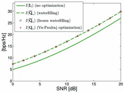
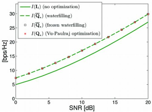
In the simulations featured in Figure 1(a) (respectively in Figure 1(b)), we consider a MIMO system with $r=t=4$ (respectively $r=t=8$). In both figures, we have represented the average mutual information $I({\mathbf{I}}_t)$ (i.e., without optimization), the optimal average mutual information $I({\overline{\mathbf{Q}}}_{*})$ (i.e., with an input covariance matrix maximizing the approximation $\overline{I}$) obtained by the iterative water-filling introduced in [11,12] (also called frozen water-filling [15]) and the same quantity $I({\overline{\mathbf{Q}}}_{*})$ obtained this time by the water-filling introduced by [15]. All the mutual information are evaluated by Monte-Carlo simulations with $20000$ channel realizations. All the values given by iterative algorithms are calculated with a relative precision of ${10}^{-3}$. The average mutual information $I({\mathbf{Q}}_{*})$ obtained with the Vu–Paulraj direct approach [2] is also represented as a reference.

Figure 1. Comparison with Vu–Paulraj algorithm.

Figure 1. Comparison with Vu–Paulraj algorithm.

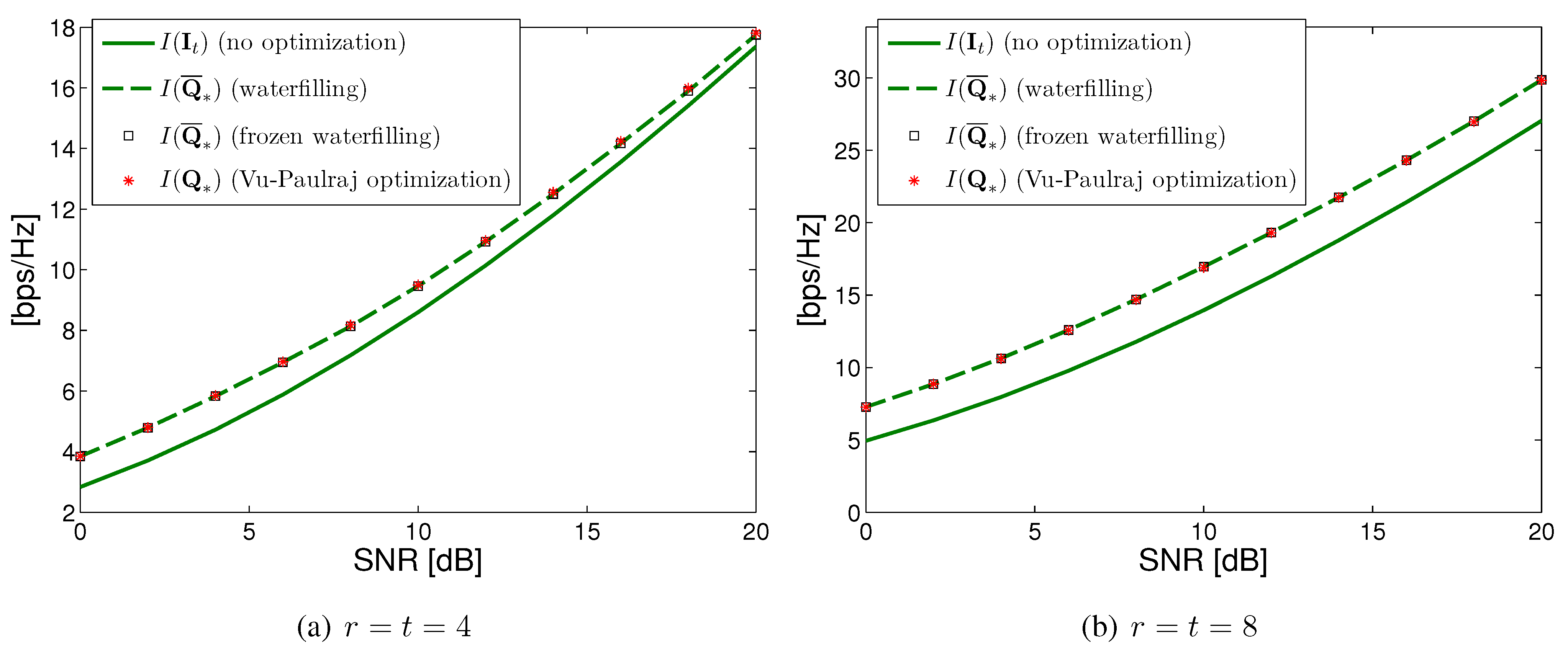
Vu–Paulraj’s algorithm is a direct approach to optimize $I(\mathbf{Q})$. It is composed of two nested iterative loops. The inner loop evaluates ${\mathbf{Q}}_{*}^{(n)}=\mathrm{argmax}\left\{I(\mathbf{Q})+k_{\mathrm{barrier}}log\det \mathbf{Q}\right\}$ thanks to the Newton algorithm with the constraint $\frac{1}{t}\mathrm{Tr}\mathbf{Q}=1$, for a given value of $k_{\mathrm{barrier}}$ and a given starting point ${\mathbf{Q}}_0^{(n)}$. Maximizing $I(\mathbf{Q})+k_{\mathrm{barrier}}log\det \mathbf{Q}$ instead of $I(\mathbf{Q})$ ensures that $\mathbf{Q}$ remains positive semi-definite through the steps of the Newton algorithm; this is the so-called barrier interior-point method. The outer loop then decreases $k_{\mathrm{barrier}}$ by a certain constant factor μ and gives the inner loop the next starting point ${\mathbf{Q}}_0^{(n+1)}={\mathbf{Q}}_{*}^{(n)}$. The algorithm stops when the desired precision is obtained, or, as the Newton algorithm requires heavy Monte-Carlo simulations for the evaluation of the gradient and of the Hessian of $I(\mathbf{Q})$, when the number of iterations of the outer loop reaches a given number $N_{max}$. As in [2], we chose $N_{max}=10$, $\mu =100$, $20000$ trials for the Monte-Carlo simulations, and we started with $k_{\mathrm{barrier}}=\frac{1}{100}$.

Both Figure 1(a) and Figure 1(b) show that maximizing $\overline{I}(\mathbf{Q})$ over the input covariance leads to significant improvement of $I(\mathbf{Q})$. All the approaches provide the same results: the two water-filling procedures presented in this section and the Vu–Paulraj’s direct approach all produce the same results, confirming the stated results.

Nonetheless, the execution times differ considerably from one algorithm to another. The indirect approaches are computationally much more efficient: in Vu–Paulraj’s algorithm, the evaluation of the gradient and of the Hessian of $I(\mathbf{Q})$ needs heavy Monte-Carlo simulations, thus slowing down drastically the calculations. Besides, the water-filling introduced by [8] is computationally slightly more efficient than the so-called frozen water-filling. Instead of two nested iterative loops (the outer to optimize the input covariance matrix $\mathbf{Q}$, the inner to solve the canonical equations), there is only one loop performing both calculations. For the present case with $r=t=8$, an average of 39.7 fixed point iterations is needed for the frozen water-filling to converge, whereas the water-filling introduced by [8] needs only 7.9 fixed point iterations on average. Table 2 illustrates these comparisons; for the three algorithms the average execution time to obtain the input covariance matrix is given, on a 2.93 GHz Intel Core 2 Duo CPU with 4 GB of RAM, for both $r=t=4$ and $r=t=8$.

Table 2. Average execution time.

	$r=t=4$	$r=t=8$
Vu–Paulraj	$503s$	$1877s$
Frozen Water-filling	$17.3ms$	$20.1ms$
Water-filling of [8]	$5.10ms$	$7.13ms$

Table 2. Average execution time.

	$r=t=4$	$r=t=8$
Vu–Paulraj	$503s$	$1877s$
Frozen Water-filling	$17.3ms$	$20.1ms$
Water-filling of [8]	$5.10ms$	$7.13ms$

6. Concluding Remarks

In this paper, we have given a comprehensive introduction to the evaluation of the capacity achieving covariance matrices of MIMO channels using large system approximation approaches. When the MIMO channel is available at the receiver and its probability distribution is available at the transmitter, the direct maximization of the mutual information w.r.t. the input covariance matrix leads to high complexity algorithms using intensive Monte-Carlo simulations. An alternative approach consists in approximating the mutual information in the large number of antennas regime and optimizing the approximation. We have recalled how it is possible to derive the large system approximations in the context of a number of MIMO channels, and have addressed their optimization. We have emphasized on important methodological points that are not necessarily covered by the existing literature, such as the strict concavity of the approximation, the structure of the argument of its maximum, the accuracy of the large system approach w.r.t. the number of antennas, and the justification of iterative water-filling optimization algorithms. We finally mention that the mutual information considered in this paper allow to obtain insights on the performances of MIMO systems equipped with maximum likelihood receivers. As these receivers may be complex to implement, reduced complexity schemes such as the minimum mean squares (MMSE) receivers are often considered. In this context, the relevant mutual information to be optimized versus the input precoder is different, and is defined as the sum over the transmit antennas of terms $\mathbb{E}(log(1+{\beta }_j))$ where ${\beta }_j$ represents the output MMSE signal to interference plus noise ratio associated to the stream sent by antenna j. The corresponding optimization problems are more difficult because they are not convex as in the context of the present paper. However, high accuracy large system approximation techniques can still be developed (see e.g., [28,29]), and provide both insights on the optimal precoders and low complexity maximization algorithms. The case of Rayleigh bi-correlated MIMO channels was recently addressed in [30] where the structure of the optimal precoders was analyzed. However, an important work remains to be done in the context of the other usual MIMO channels.

References

- Telatar, E. Capacity of multi-antenna gaussian channels. Eur. Trans. Telecommun. 1999, 10, 585–595. [Google Scholar] [CrossRef]
- Vu, M.; Paulraj, A. Capacity Optimization for Rician Correlated MIMO Wireless Channels. In Proceedings of the Thirty-Ninth Asilomar Conference on the Signals, Systems and Computers, Pacific Grove, CA, USA, November 2005; pp. 133–138.
- Goldsmith, A.; Jafar, S.; Jindal, N.; Vishwanath, S. Capacity limits of MIMO channels. IEEE J. Select. Areas Commun. 2003, 21, 684–702. [Google Scholar] [CrossRef]
- Jafar, S.; Goldsmith, A. Transmitter optimization and optimality of beamforming for multiple antenna systems. IEEE Trans. Wirel. Commun. 2004, 3, 1165–1175. [Google Scholar] [CrossRef]
- Hosli, D.; Kim, Y.; Lapidoth, A. Monotonicity results for coherent MIMO Rician channels. IEEE Trans. Inform. Theory 2005, 51, 4334–4339. [Google Scholar] [CrossRef]
- Moustakas, A.; Simon, S.; Sengupta, A. MIMO capacity through correlated channels in the presence of correlated interferers and noise: A (not so) large N analysis. IEEE Trans. Inf. Theory 2003, 49, 2545–2561. [Google Scholar] [CrossRef]
- Moustakas, A.; Simon, S. On the outage capacity of correlated multiple-path MIMO channels. IEEE Trans. Inf. Theory 2007, 53, 3887. [Google Scholar] [CrossRef]
- Taricco, G. Asymptotic mutual information statistics of separately correlated Rician fading MIMO channels. IEEE Trans. Inf. Theory 2008, 54, 3490–3504. [Google Scholar] [CrossRef]
- Wen, C.; Jin, S.; Wong, K.; Chen, J.; Ting, P. On the Ergodic Capacity of Jointly-Correlated Rician Fading MIMO Channels. In Proceedings of IEEE International Conference on Acoustics, Speech and Signal, Prague, Czech Republic, May 2011; pp. 3224–3227.
- Tulino, A.; Verdú, S. Random Matrix Theory and Wireless Communications; Now Publishers Inc: Hanover, MA, USA, 2004. [Google Scholar]
- Dumont, J.; Hachem, W.; Lasaulce, S.; Loubaton, P.; Najim, J. On the capacity achieving covariance matrix for Rician MIMO channels: An asymptotic approach. IEEE Trans. Inf. Theory 2010, 56, 1048–1069. [Google Scholar] [CrossRef]
- Dupuy, F.; Loubaton, P. On the capacity achieving covariance matrix for frequency selective MIMO channels using the asymptotic approach. Inf. Theory IEEE Trans. 2011, 57, 5737–5753. [Google Scholar] [CrossRef] [Green Version]
- Couillet, R.; Debbah, M.; Silverstein, J. A deterministic equivalent for the analysis of correlated MIMO multiple access channels. IEEE Trans. Inf. Theory 2011, 57, 3493–3514. [Google Scholar] [CrossRef]
- Wen, C.; Ting, P.; Chen, J. Asymptotic analysis of MIMO wireless systems with spatial correlation at the receiver. IEEE Trans. Commun. 2006, 54, 349–363. [Google Scholar] [CrossRef]
- Taricco, G.; Riegler, E. On the ergodic capacity of correlated Rician fading MIMO channels with interference. IEEE Trans. Inf. Theory 2011, 57, 4123–4137. [Google Scholar] [CrossRef]
- Wen, C.; Jin, S.; Wong, K. On the sum-rate of multiuser MIMO uplink channels with jointly-correlated Rician fading. IEEE Trans. Commun. 2011, 59, 2883–2895. [Google Scholar] [CrossRef]
- Luenberger, D. Optimization by Vector Space Methods; John Wiley and Sons: New York, NY, USA, 1969. [Google Scholar]
- Marčenko, V.; Pastur, L. Distribution of eigenvalues for some sets of random matrices. Math. USSR Sb. 1967, 1, 457. [Google Scholar] [CrossRef]
- Pastur, L.; Shcherbina, M. Eigenvalue Distribution of Large Random Matrices. In Mathematical Surveys and Monographs; American Mathematical Society: Providence, RI, USA, 2011. [Google Scholar]
- Bai, Z.; Silverstein, J. Spectral Analysis of Large Dimensional Random Matrices (Springer Series in Statistics), 2nd ed.; Springer: Heidelberg, Germnay, 2009. [Google Scholar]
- Girko, V. Theory of Stochastic Canonical Equations, Volume I; Kluwer Academic Publishers: Dordrecht, The Netherlands, 2001; Chapter 7. [Google Scholar]
- Taricco, G. On the Capacity of Separately-Correlated MIMO Rician Channels. In Proceedings of Global Telecommunications Conference, San Francisco, CA, USA, December 2006.
- Sayeed, A. Deconstructing multiantenna fading channels. IEEE Trans. Signal Process. 2002, 50, 2563–2579. [Google Scholar] [CrossRef]
- Hachem, W.; Loubaton, P.; Najim, J. Deterministic equivalents for certain functionals of large random matrices. Ann. Appl. Probab. 2007, 17, 875–930. [Google Scholar] [CrossRef]
- Borwein, J.; Lewis, A. Convex Analysis and Nonlinear Optimization : Theory and Examples; Springer: Verlag, Germany, 2000. [Google Scholar]
- Boyd, S.; Vandenberghe, L. Convex Optimization; Cambridge University Press: Cambridge, UK, 2004. [Google Scholar]
- Bolcskei, H.; Gesbert, D.; Paulraj, A. On the capacity of OFDM-based spatial multiplexing systems. IEEE Trans. Commun. 2002, 50, 225–234. [Google Scholar] [CrossRef]
- Kumar, K.; Caire, G.; Moustakas, A. Asymptotic performance of linear receivers in MIMO fading channels. IEEE Trans. Inf. Theory 2009, 55, 4398–4418. [Google Scholar] [CrossRef]
- Moustakas, A.; Kumar, K.; Caire, G. Performance of MMSE MIMO Receivers: A Large N analysis for Correlated Channels. In Proceedings of IEEE Vehicular Technology Conference, Barcelona, Spain, 2009.
- Artigue, C.; Loubaton, P. On the precoder design of flat fading MIMO systems equipped with MMSE receivers: A large system approach. IEEE Trans. Inf. Theory 2011, 57, 4138–4155. [Google Scholar] [CrossRef]
© 2012 by the authors licensee MDPI, Basel, Switzerland. This article is an open access article distributed under the terms and conditions of the Creative Commons Attribution license ( http://creativecommons.org/licenses/by/3.0/).
Share and Cite
MDPI and ACS Style
Dupuy, F.; Loubaton, P. Optimization of MIMO Systems Capacity Using Large Random Matrix Methods. Entropy 2012, 14, 2122-2142. https://doi.org/10.3390/e14112122
AMA Style
Dupuy F, Loubaton P. Optimization of MIMO Systems Capacity Using Large Random Matrix Methods. Entropy. 2012; 14(11):2122-2142. https://doi.org/10.3390/e14112122
Chicago/Turabian StyleDupuy, Florian, and Philippe Loubaton. 2012. "Optimization of MIMO Systems Capacity Using Large Random Matrix Methods" Entropy 14, no. 11: 2122-2142. https://doi.org/10.3390/e14112122