The Extension of Statistical Entropy Analysis to Chemical Compounds

Abstract

Statistical entropy analysis (SEA) quantifies the dilution and concentration of conservative substances (e.g., heavy metals) in a system. In this paper, the SEA concept is extended (eSEA) to make it applicable to systems in which the chemical speciation is of particular importance. The eSEA is applied to a simplified region used for crop farming. The extent to which the region concentrates or dilutes nitrogen compounds is expressed as the change in statistical entropy (ΔH). A detailed derivation for the calculation of ΔH is provided. The results are discussed for four variations of the crop farming system, showing that the efficiency of crop farming can be expressed by eSEA.

1. Introduction

Developed in the 1980s, material flow analysis (MFA) is a technique that tracks the flows of goods and substances between processes and through a defined system [1]. Processes that transform input goods into different output goods concentrate and dilute various substances. Concentration usually occurs when products and byproducts are manufactured from raw materials, wastes are collected or materials are recovered from waste. Dilution occurs when materials are mixed (as in the fabrication of complex products) or emissions are released to the environment. With regard to material management, concentration is generally considered as a positive and beneficial process because it increases the availability of a material. Dilution, however, is easier to accomplish than concentration, although it represents a disadvantage due to increased expenses for material recovery. On the other hand, a certain degree of dilution is acceptable as long as it complies with environmental protection regulations. Such concentration and dilution phenomena can be quantified by Statistical Entropy Analysis (SEA) [2,3]. SEA is based on Shannon’s definition for statistical entropy in information technology [4]. The probability of an event is transformed into the probability of appearance of a chemical element, expressed by its concentration. Therewith, statistical entropy becomes a tool used to quantify the distribution of conservative substances (e.g., particular chemical elements such as heavy metals) and it is a tailor-made evaluation tool for MFA studies (in the following, we use MFA terminology; term definitions can be found in [5]).

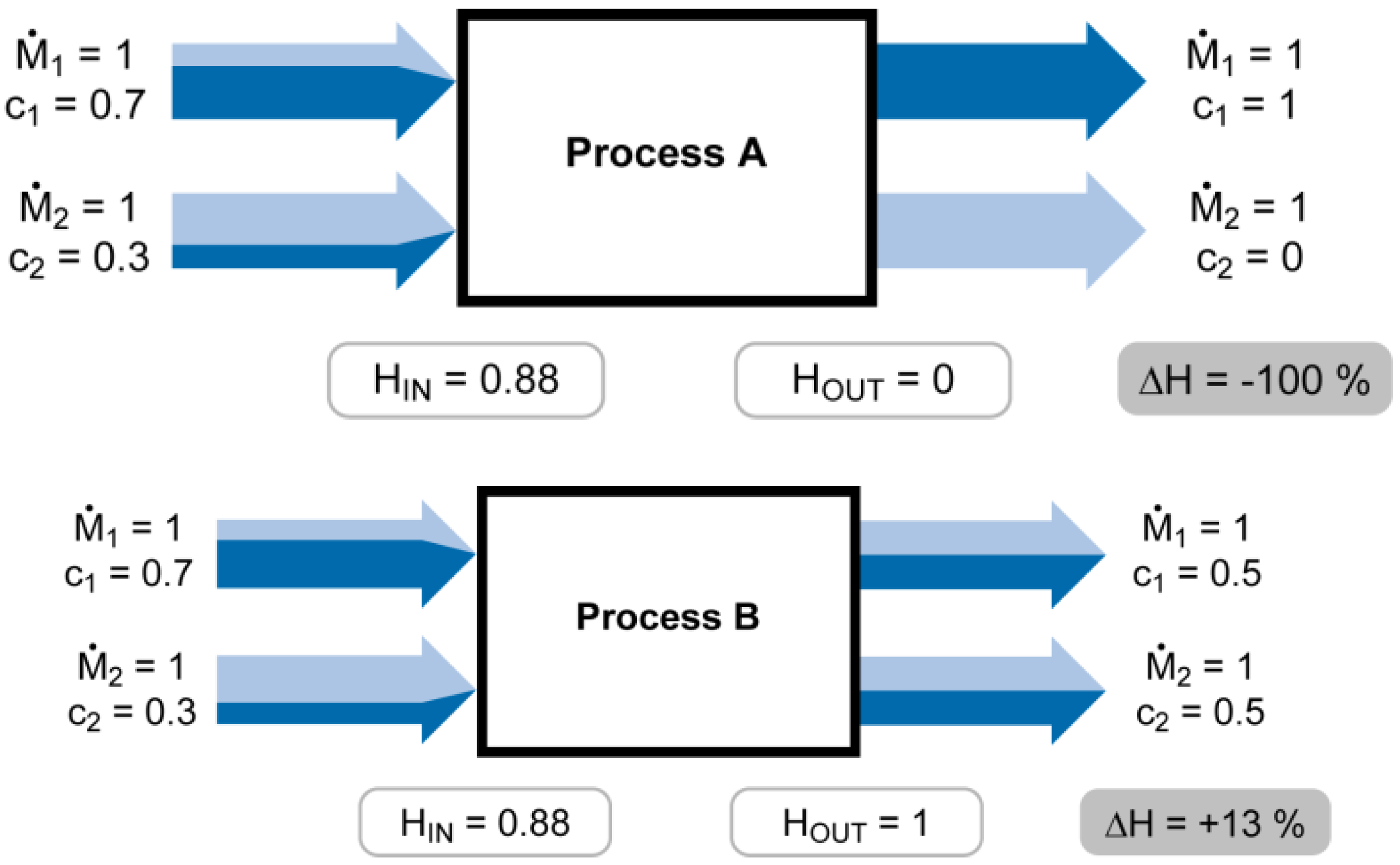
SEA can be illustrated through a simple cadmium budget of a process with two input flows that are transformed into two output flows (see Figure 1). Each flow is described by a mass flow rate ($\dot{\mathrm{M}}$) and the respective concentration of cadmium (c). In a first step we assume $\dot{\mathrm{M}}=1$ and replace the probabilities in Shannon’s entropy formula [Equations (1) and (2)] by concentrations [Equations (3) and (4)]. If the concentration in a flow is 100%, then the probability to find cadmium in it is 100%. Equation 3 is applied to the input (H_IN) and the output (H_OUT) of the process and the change is expressed as $\Delta \mathrm{H}={\mathrm{H}}_{\text{OUT}}-{\mathrm{H}}_{\text{IN}}$(in Thermodynamics the letter “H” is used for enthalpy while “S” designates entropy. However, we use “H” to make clear that entropy as applied here is derived from statistical entropy where “H” is used):

$$\mathrm{H}=-{\displaystyle \sum _{\mathrm{i}=1}^{\mathrm{k}}{\mathrm{P}}_{\mathrm{i}}*{\log }_2\left({\mathrm{P}}_{\mathrm{i}}\right)}$$

(1)

$${\displaystyle \sum _{\mathrm{i}=1}^{\mathrm{k}}{\mathrm{P}}_{\mathrm{i}}=1}$$

(2)

$$\mathrm{H}({\mathrm{c}}_{\mathrm{i}})=-{\displaystyle \sum _{\mathrm{i}=1}^{\mathrm{k}}{\mathrm{c}}_{\mathrm{i}}*{\log }_2({\mathrm{c}}_{\mathrm{i}})}$$

(3)

$${\displaystyle \sum _{\mathrm{i}=1}^{\mathrm{k}}{\mathrm{c}}_{\mathrm{i}}=1}$$

(4)

According to Shannon the maximum entropy is given for the equiprobability of all possible configurations:

$${\mathrm{H}}_{\max }={\log }_2(\mathrm{k})$$

(5)

Transferred to the simple example in Figure 1, maximum entropy occurs if cadmium is equally distributed among the output flows (cf. Figure 1, Process B).

Figure 1. Simple cadmium budget of a process with two input flows that are transformed into two output flows. All mass flow rates $\dot{\mathrm{M}}=1$, the colors indicate the concentrations of cadmium. Process A achieves maximum concentrating of cadmium (H_OUT = 0). Process B realizes the equal distribution of cadmium to both flows and H_OUT = H_max = 1.

Figure 1. Simple cadmium budget of a process with two input flows that are transformed into two output flows. All mass flow rates $\dot{\mathrm{M}}=1$, the colors indicate the concentrations of cadmium. Process A achieves maximum concentrating of cadmium (H_OUT = 0). Process B realizes the equal distribution of cadmium to both flows and H_OUT = H_max = 1.

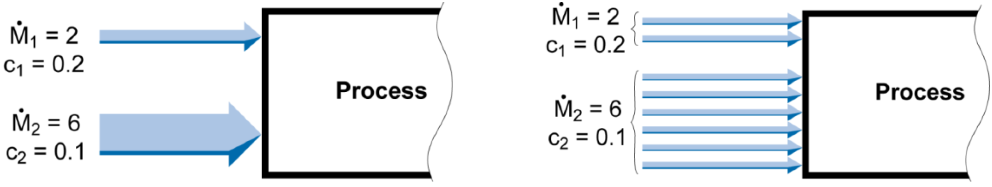
However, for real processes $\dot{\mathrm{M}}\ne 1$ and the mass flow rates of the flows have to be considered, as it makes a difference if it is high or low. To consider $\dot{\mathrm{M}}$ the mass flow rate is interpreted as a frequency of occurrence: From a materials point of view a flow with $\dot{\mathrm{M}}=6$ is the same as 6 flows with $\dot{\mathrm{M}}=1$ (cf. Figure 2). The basic statistical entropy formula for the distribution of a substance in different material flows is then:

$$\mathrm{H}({\dot{\mathrm{M}}}_{\mathrm{i}},{\mathrm{c}}_{\mathrm{i}})=-{\displaystyle \sum _{\mathrm{i}=1}^{\mathrm{k}}{\dot{\mathrm{M}}}_{\mathrm{i}}*{\mathrm{c}}_{\mathrm{i}}*{\log }_2({\mathrm{c}}_{\mathrm{i}})}$$

(6)

$${\displaystyle \sum _{\mathrm{i}=1}^{\mathrm{k}}{\dot{\mathrm{M}}}_{\mathrm{i}}*{\mathrm{c}}_{\mathrm{i}}=1}$$

(7)

$${\mathrm{H}}_{\max }={\log }_2\left({\displaystyle \sum _{\mathrm{i}=1}^{\mathrm{k}}{\dot{\mathrm{M}}}_{\mathrm{i}}}\right)$$

(8)

Figure 2. The real mass flow rates are interpreted as the frequency of occurrence of flows with $\dot{\mathrm{M}}=1$.

Figure 2. The real mass flow rates are interpreted as the frequency of occurrence of flows with $\dot{\mathrm{M}}=1$.

SEA has been applied to the European copper cycle, demonstrating that SEA can be applied to systems consisting of several processes, that a real system is a succession of concentration and dilution processes, and finally, that SEA is a powerful indicator for quantifying the quality of material management of processes and systems [3]. Further applications of SEA are reported in [7] and [8].

Classical MFA addresses chemical elements (e.g., heavy metals or nutrients such as nitrogen or phosphorous). However, the chemical speciation of an element is often important to model. For instance, a simple nitrogen (N) balance of a Waste-to-Energy (WtE) plant is of limited value because it is important to know whether the nitrogen leaves the plant as molecular nitrogen (N₂), nitrous oxide (NO, NO₂), ammonia (NH₃), nitrate (NO₃⁻) or some other form. Therefore, in this paper, we want to extend the “classical” SEA to make it applicable to chemical compounds. To demonstrate how the extended Statistical Entropy Analysis (eSEA) is calculated and how the results can be used, we apply the method to a simplified hypothetical system consisting of a crop farming region that transforms nitrogen compounds. The aim of this paper is to introduce the extended SEA and demonstrate its application to a simple system. The focus is not on an actual crop farming region.

2. Description of the Investigated System and Data

The investigated system is simple and consists of one process (crop farming), four input material flows (mineral fertilizer, seeds, deposition, and N-fixation), and four output material flows (plant-based agricultural product, losses to the atmosphere, groundwater, and surface water) transforming various nitrogen compounds (e.g., CO(NH₂)₂, NO₃, NH₄, N₂, NO_x, and N₂O), as shown in Figure 3a (base system S0). The system represents a hypothetical region where crop farming is practiced. This farming region yields a product (plant-derived protein expressed as organically bound nitrogen, N_org). Different processes are used to describe the nitrogen transformation and transport. Deposition in the form of rain and snow usually brings nitrate (NO₃⁻) and ammonium (NH₄⁺) into the region. N₂ is adsorbed and then oxidized by microorganisms, resulting in higher nitrogen availability in the soil (N-fixation). Emissions to ground and surface water typically occur as nitrate (NO₃⁻), ammonium (NH₄⁺), and organic nitrogen (N_org). Mineral fertilizer is assumed to be a mixture of urea [CO(NH₂)₂] and ammonium nitrate (NH₄NO₃), and seeds contain organically bound nitrogen (N_org) in the form of protein. Gaseous losses are mostly ammonia (NH₃), elemental nitrogen (N₂) and, to a lesser extent, nitrous oxide (N₂O) and other oxides of nitrogen (NO_x) (see Figure 3).

Data are taken from a study on nutrient balances for Austria and Hungary [9]. All data correspond to an area of 1 hectare and a time scale of 1 year. In this way, regions of different dimensions can be compared to each other.

In this paper, three explicit system variations are selected to demonstrate how the eSEA works. Practical implications of these emissions scenarios are not the focus of this work. In variations V1 and V2, the gaseous emissions are modified. In variation V3, the emissions to surface and groundwater are changed. However, the system’s total nitrogen throughput always remains the same. Figure 3b presents variation V1. In this variation, the gaseous emissions of NH₃, N₂O and NO_x are each reduced by 50% relative to the original system S0 for the benefit of N₂ (cf. Figure 3a). In the second variation (V2), the gaseous emissions of NH₃, N₂O and NO_x are each increased by 50% relative to the base system S0, and the emission of N₂ is reduced accordingly (cf. Figure 3c). Finally, a variation is created (V3) in which the emissions to surface and groundwater are decreased by 50% for the benefit of the product (cf. 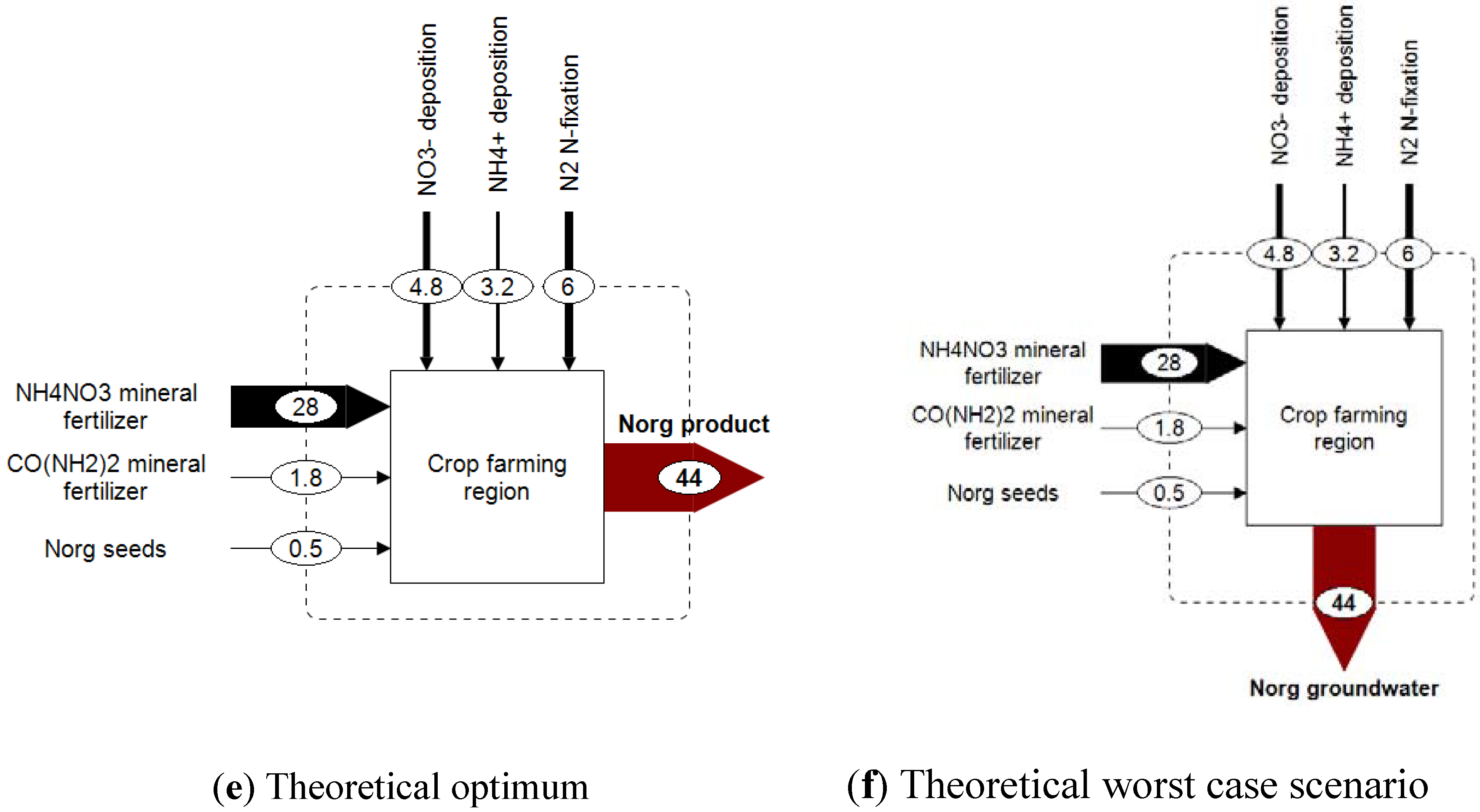Figure 3d). To classify the eSEA results, both an optimal and a worst case scenario are introduced as well. Both scenarios are highly fictitious, but they serve as a reference. Optimal nitrogen management in our exemplary region would mean that all nitrogen is transferred into the farming product (cf. Figure 3e). In this case, the eSEA yields the best result, which is minimal entropy production or, in other words, minimal dilution. In the theoretical worst case scenario, the nitrogen that comes into the region is transformed to organic nitrogen and emitted to groundwater (Figure 3f). This scenario yields the worst result, which is equivalent to maximum entropy generation or maximum dilution. High entropy generation occurs if a nitrogen compound is emitted into an environmental compartment with a low natural background concentration of that particular nitrogen compound (see Section 3.3).

Figure 3. Nitrogen budgets for a hypothetical and simplified crop farming region based on Austrian data (data rounded); all values are given in kgN/ha/yr.

Figure 3. Nitrogen budgets for a hypothetical and simplified crop farming region based on Austrian data (data rounded); all values are given in kgN/ha/yr.

3. Extension of the Statistical Entropy Analysis (eSEA)

For a comprehensive derivation of the SEA (formulas and assumptions), see Rechberger and colleagues [2,3,10]. The extension of the SEA to chemical compounds (eSEA) is based on the equations given in [2] and [10] and is explained on the basis of the hypothetical crop farming system presented above (cf. Figure 3). Therefore, the most important principles of the SEA are addressed in this paper and the main equations are contrasted with the equations of the extended SEA (see Table 1).

The mass balance principle requires that the total amount of incoming nitrogen equals the total amount of nitrogen that is leaving the system, assuming that there is no storage of nitrogen compounds in the region (i.e., steady-state conditions; storage phenomena are not considered here but could be considered as shown in [3]). The mass flows (such as the amounts of rainwater, fertilizer, and product) indicated by ${\dot{\mathrm{m}}}_{\text{i}}$ (index i for flows), and the concentrations of the individual nitrogen compounds (c_im, index m for compounds) are the required basic data. Concentrations of nitrogen compounds are used as concentrations of pure nitrogen in a particular mass flow. A description of all indices and parameters (including their physical units) is given at the end of the paper. Before the statistical entropy can be calculated, some simple normalization steps are required to convert these data (${\dot{\mathrm{m}}}_{\text{i}}$, c_im) into corresponding dimensionless values. This allows for a comparison of systems of different sizes. First, the nitrogen loads (${\dot{\mathrm{X}}}_{\text{im}}$) for all nitrogen compounds in a particular material flow in the input and output are computed according to Equation (9):

$${\dot{\mathrm{X}}}_{\mathrm{i}\mathrm{m}}={\dot{\mathrm{M}}}_{\mathrm{i}}*{\mathrm{c}}_{\mathrm{i}\mathrm{m}}$$

(9)

$${\mathrm{m}}_{\mathrm{i}}=\frac{{\dot{\mathrm{M}}}_{\mathrm{i}}}{{\displaystyle \sum _{\mathrm{i}=1}^{\mathrm{k}}{\displaystyle \sum _{\mathrm{m}=1}^{\mathrm{r}}{\dot{\mathrm{X}}}_{\mathrm{i}\mathrm{m}}}}}$$

(10)

where k is the number of input material flows (here, k = 4: fertilizer, seeds, deposition, N-fixation), and r is the number of different nitrogen compounds that appear in the input flows [here, r=6: NH₄⁺, NO₃⁻, CO(NH₂)₂, NH₄NO₃, N_org, N₂].

The denominator of Equation (10) is the total flow of nitrogen through the system, so the specific masses m_i are related to one mass-unit of nitrogen (e.g., kg fertilizer input per kg total nitrogen throughput).

Next, the specific loads X_im that describe the fractions of each nitrogen compound with respect to the total nitrogen in the different material flows are calculated as:

$${\mathrm{X}}_{\mathrm{i}\mathrm{m}}={\mathrm{m}}_{\mathrm{i}}*{\mathrm{c}}_{\mathrm{i}\mathrm{m}}$$

(11)

The sum of all specific nitrogen loads for each nitrogen compound must be 100% for both the input and output (mass balance principle). In mathematical terms, we have:

$${\displaystyle \sum _{\mathrm{i}=1}^{\mathrm{k}}{\displaystyle \sum _{\mathrm{m}=1}^{\mathrm{r}}{\mathrm{X}}_{\mathrm{i}\mathrm{m}}^{\mathrm{I}\mathrm{N}}=1}}$$

(12)

$${\displaystyle \sum _{\mathrm{i}=1}^{\mathrm{l}}{\displaystyle \sum _{\mathrm{m}=1}^{\mathrm{s}}{\mathrm{X}}_{\mathrm{i}\mathrm{m}}^{\mathrm{O}\mathrm{U}\mathrm{T}}=1}}$$

(13)

where $\text{l}$ is the number of all outgoing material flows (here, $\text{l }$= 4: product and losses to the atmosphere, groundwater, and surface water), and s represents the number of nitrogen compounds in the output (here, s = 7: NO₃⁻, NH₄⁺, N_org, NH₃, NO_x, N₂O, N₂). The definitions of k and r are as given above.

3.1. Estimation of the Statistical Entropy of the Input (H_IN)

The extended statistical entropy is first calculated for the nitrogen input into the system. In reference to the system presented in this work, statistical entropy of the input is the sum of the statistical entropy values for CO(NH₂)₂ and NH₄NO₃ in the mineral fertilizer, N_org in the seeds, NH₄⁺ and NO₃⁻ from deposition, and N₂ from N-fixation. The equivalent for the SEA would be the sum of the statistical entropy values for the total nitrogen from the mineral fertilizer, seeds, deposition, and N-fixation with no differentiation among N species (see Table 1).

Table 1. Calculation of the statistical entropy for the input; left side: classical SEA; right side: extended SEA.

SEA	eSEA
$${\mathrm{H}}_{\mathrm{I}\mathrm{N},\mathrm{N}}({\mathrm{m}}_{\mathrm{i}},{\mathrm{c}}_{\mathrm{i}\mathrm{N}})=-{\displaystyle \sum _{\mathrm{i}=1}^{\mathrm{k}}{\mathrm{m}}_{\mathrm{i}}*{\mathrm{c}}_{\mathrm{i}\mathrm{N}}*{\log }_2({\mathrm{c}}_{\mathrm{i}\mathrm{N}})}$$ (14)	$${\mathrm{H}}_{\mathrm{I}\mathrm{N}}({\mathrm{m}}_{\mathrm{i}},{\mathrm{c}}_{\mathrm{i}\mathrm{m}})=-{\displaystyle \sum _{\mathrm{i}=1}^{\mathrm{k}}{\displaystyle \sum _{\mathrm{m}=1}^{\mathrm{r}}{\mathrm{m}}_{\mathrm{i}}*{\mathrm{c}}_{\mathrm{i}\mathrm{m}}*{\log }_2({\mathrm{c}}_{\mathrm{i}\mathrm{m}})}}$$ (15)
Entropy is a function of the total nitrogen load (N) in the different input flows	Entropy is a function of the load of all nitrogen compounds (m) that appear in the different input flows

Table 1. Calculation of the statistical entropy for the input; left side: classical SEA; right side: extended SEA.

SEA	eSEA
$${\mathrm{H}}_{\mathrm{I}\mathrm{N},\mathrm{N}}({\mathrm{m}}_{\mathrm{i}},{\mathrm{c}}_{\mathrm{i}\mathrm{N}})=-{\displaystyle \sum _{\mathrm{i}=1}^{\mathrm{k}}{\mathrm{m}}_{\mathrm{i}}*{\mathrm{c}}_{\mathrm{i}\mathrm{N}}*{\log }_2({\mathrm{c}}_{\mathrm{i}\mathrm{N}})}$$ (14)	$${\mathrm{H}}_{\mathrm{I}\mathrm{N}}({\mathrm{m}}_{\mathrm{i}},{\mathrm{c}}_{\mathrm{i}\mathrm{m}})=-{\displaystyle \sum _{\mathrm{i}=1}^{\mathrm{k}}{\displaystyle \sum _{\mathrm{m}=1}^{\mathrm{r}}{\mathrm{m}}_{\mathrm{i}}*{\mathrm{c}}_{\mathrm{i}\mathrm{m}}*{\log }_2({\mathrm{c}}_{\mathrm{i}\mathrm{m}})}}$$ (15)
Entropy is a function of the total nitrogen load (N) in the different input flows	Entropy is a function of the load of all nitrogen compounds (m) that appear in the different input flows

3.2. Estimation of the Statistical Entropy of the Output (H_OUT)

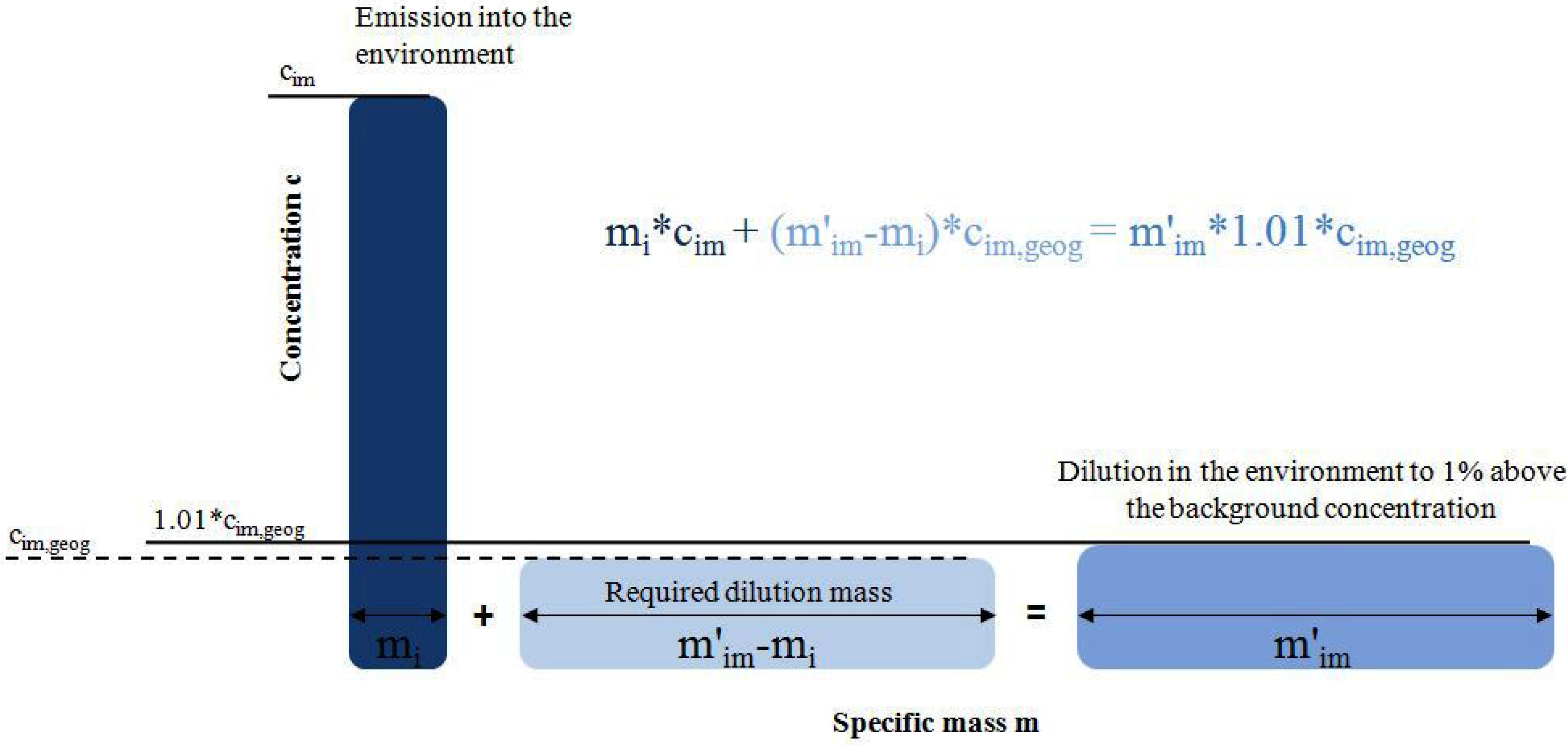
Nitrogen that is not transferred to a solid product is either diluted in the atmosphere (gaseous losses) or in the hydrosphere (surface and groundwater) in the form of different nitrogen compounds. Dilution leads to an entropy increase. This is considered in the calculations by the assumption that the emissions are diluted up to a concentration that is 1% above the corresponding background concentration (c_im,geog) in the receiving environmental compartment (cf. Figure 4; see Equations 18–21 in Table 2). It has been shown that this assumption represents the real dilution process with sufficient accuracy [10].

Figure 4. Illustration of the dilution process of an emission.

Figure 4. Illustration of the dilution process of an emission.

Table 2. Calculation of the statistical entropy for the output; left side: classical SEA; right side: extended SEA.

SEA	eSEA
$${\mathrm{H}}_{\text{OUT},\mathrm{N}}=({\mathrm{m}}_{\mathrm{i}}^{\prime },{\mathrm{c}}_{\mathrm{i}\mathrm{N}}^{\prime })=-{\displaystyle \sum _{\mathrm{i}=1}^{\mathrm{l}}{\mathrm{m}}_{\mathrm{i}}^{\prime }*{\mathrm{c}}_{\mathrm{i}\mathrm{N}}^{\prime }*{\log }_2({\mathrm{c}}_{\mathrm{i}\mathrm{N}}^{\prime })}$$ (16)	$${\mathrm{H}}_{\mathrm{O}\mathrm{U}\mathrm{T}}({\mathrm{m}}_{\mathrm{i}\mathrm{m}}^{\prime },{\mathrm{c}}_{\mathrm{i}\mathrm{m}}^{\prime })=-{\displaystyle \sum _{\mathrm{i}=1}^{\mathrm{l}}{\displaystyle \sum _{\mathrm{m}=1}^{\mathrm{s}}{\mathrm{m}}_{\mathrm{i}\mathrm{m}}^{\prime }*{\mathrm{c}}_{\mathrm{i}\mathrm{m}}^{\prime }*{\log }_2({\mathrm{c}}_{\mathrm{i}\mathrm{m}}^{\prime })}}$$ (17)
Entropy for the output depends on total nitrogen loads (N) in the different output flows	Entropy depends on the load of all nitrogen compounds (m) that appear in the different output flows
CALCULATION OF THE DILUTING TERMS
$${\mathrm{m}}_{\mathrm{i}}^{\prime }={\mathrm{m}}_{\mathrm{i}}*\frac{{\mathrm{c}}_{\mathrm{i}\mathrm{N}}-{\mathrm{c}}_{\mathrm{i}\mathrm{N},\mathrm{g}\mathrm{e}\mathrm{o}\mathrm{g}}}{{\mathrm{c}}_{\mathrm{i}\mathrm{N},\mathrm{g}\mathrm{e}\mathrm{o}\mathrm{g}}}*100+{\mathrm{m}}_{\mathrm{i}}$$ (18)	$${\mathrm{m}}_{\mathrm{i}\mathrm{m}}^{\prime }={\mathrm{m}}_{\mathrm{i}}*\frac{{\mathrm{c}}_{\mathrm{i}\mathrm{m}}-{\mathrm{c}}_{\mathrm{i}\mathrm{m},\mathrm{g}\mathrm{e}\mathrm{o}\mathrm{g}}}{{\mathrm{c}}_{\mathrm{i}\mathrm{m},\mathrm{g}\mathrm{e}\mathrm{o}\mathrm{g}}}*100+{\mathrm{m}}_{\mathrm{i}}$$ (19)
$${\mathrm{c}}_{\mathrm{i}\mathrm{N}}^{\prime }=\frac{{\mathrm{c}}_{\mathrm{i}\mathrm{N}}*{\mathrm{c}}_{\mathrm{i}\mathrm{N},\mathrm{g}\mathrm{e}\mathrm{o}\mathrm{g}}}{{\mathrm{c}}_{\mathrm{i}\mathrm{N}}-0.99*{\mathrm{c}}_{\mathrm{i}\mathrm{N},\mathrm{g}\mathrm{e}\mathrm{o}\mathrm{g}}}*0.01$$ (20)	$${\mathrm{c}}_{\mathrm{i}\mathrm{m}}^{\prime }=\frac{{\mathrm{c}}_{\mathrm{i}\mathrm{m}}*{\mathrm{c}}_{\mathrm{i}\mathrm{m},\mathrm{g}\mathrm{e}\mathrm{o}\mathrm{g}}}{{\mathrm{c}}_{\mathrm{i}\mathrm{m}}-0.99*{\mathrm{c}}_{\mathrm{i}\mathrm{m},\mathrm{g}\mathrm{e}\mathrm{o}\mathrm{g}}}*0.01$$ (21)

Table 2. Calculation of the statistical entropy for the output; left side: classical SEA; right side: extended SEA.

SEA	eSEA
$${\mathrm{H}}_{\text{OUT},\mathrm{N}}=({\mathrm{m}}_{\mathrm{i}}^{\prime },{\mathrm{c}}_{\mathrm{i}\mathrm{N}}^{\prime })=-{\displaystyle \sum _{\mathrm{i}=1}^{\mathrm{l}}{\mathrm{m}}_{\mathrm{i}}^{\prime }*{\mathrm{c}}_{\mathrm{i}\mathrm{N}}^{\prime }*{\log }_2({\mathrm{c}}_{\mathrm{i}\mathrm{N}}^{\prime })}$$ (16)	$${\mathrm{H}}_{\mathrm{O}\mathrm{U}\mathrm{T}}({\mathrm{m}}_{\mathrm{i}\mathrm{m}}^{\prime },{\mathrm{c}}_{\mathrm{i}\mathrm{m}}^{\prime })=-{\displaystyle \sum _{\mathrm{i}=1}^{\mathrm{l}}{\displaystyle \sum _{\mathrm{m}=1}^{\mathrm{s}}{\mathrm{m}}_{\mathrm{i}\mathrm{m}}^{\prime }*{\mathrm{c}}_{\mathrm{i}\mathrm{m}}^{\prime }*{\log }_2({\mathrm{c}}_{\mathrm{i}\mathrm{m}}^{\prime })}}$$ (17)
Entropy for the output depends on total nitrogen loads (N) in the different output flows	Entropy depends on the load of all nitrogen compounds (m) that appear in the different output flows
CALCULATION OF THE DILUTING TERMS
$${\mathrm{m}}_{\mathrm{i}}^{\prime }={\mathrm{m}}_{\mathrm{i}}*\frac{{\mathrm{c}}_{\mathrm{i}\mathrm{N}}-{\mathrm{c}}_{\mathrm{i}\mathrm{N},\mathrm{g}\mathrm{e}\mathrm{o}\mathrm{g}}}{{\mathrm{c}}_{\mathrm{i}\mathrm{N},\mathrm{g}\mathrm{e}\mathrm{o}\mathrm{g}}}*100+{\mathrm{m}}_{\mathrm{i}}$$ (18)	$${\mathrm{m}}_{\mathrm{i}\mathrm{m}}^{\prime }={\mathrm{m}}_{\mathrm{i}}*\frac{{\mathrm{c}}_{\mathrm{i}\mathrm{m}}-{\mathrm{c}}_{\mathrm{i}\mathrm{m},\mathrm{g}\mathrm{e}\mathrm{o}\mathrm{g}}}{{\mathrm{c}}_{\mathrm{i}\mathrm{m},\mathrm{g}\mathrm{e}\mathrm{o}\mathrm{g}}}*100+{\mathrm{m}}_{\mathrm{i}}$$ (19)
$${\mathrm{c}}_{\mathrm{i}\mathrm{N}}^{\prime }=\frac{{\mathrm{c}}_{\mathrm{i}\mathrm{N}}*{\mathrm{c}}_{\mathrm{i}\mathrm{N},\mathrm{g}\mathrm{e}\mathrm{o}\mathrm{g}}}{{\mathrm{c}}_{\mathrm{i}\mathrm{N}}-0.99*{\mathrm{c}}_{\mathrm{i}\mathrm{N},\mathrm{g}\mathrm{e}\mathrm{o}\mathrm{g}}}*0.01$$ (20)	$${\mathrm{c}}_{\mathrm{i}\mathrm{m}}^{\prime }=\frac{{\mathrm{c}}_{\mathrm{i}\mathrm{m}}*{\mathrm{c}}_{\mathrm{i}\mathrm{m},\mathrm{g}\mathrm{e}\mathrm{o}\mathrm{g}}}{{\mathrm{c}}_{\mathrm{i}\mathrm{m}}-0.99*{\mathrm{c}}_{\mathrm{i}\mathrm{m},\mathrm{g}\mathrm{e}\mathrm{o}\mathrm{g}}}*0.01$$ (21)

To calculate the statistical entropy for gaseous (NH₃, N₂, NO_x, N₂O) and aqueous emissions (NH₄⁺, NO₃⁻, N_org), the specific masses m_i from Equation (10) are replaced by so-called diluting masses (see Equation (19) in Table 2). The corresponding specific concentrations are given by Equation (21). The atmospheric background concentrations used in this paper are taken as the mean values from the ESPERE Climate Encyclopedia [11]. Both the NO₃⁻ and NH₄⁺ background concentrations in surface and groundwater are set in accordance with the good ecological status of water bodies according to the Austrian Water Act [12,13,14]. Organically bound nitrogen is rarely present in the hydrosphere, so its background concentration is assumed to be approximately four orders of magnitude smaller than the background concentration for NH₄⁺. In principle, other reference concentrations could be used to perform the eSEA, such as eco-toxicological safety values. In this case, the result could be interpreted as eco-toxicological harming potential. Such an approach has not yet been systematically investigated. For nitrogen in the product, no further dilution is considered because consumption and use are not part of the investigated system.

3.3. Estimation of the Maximum Statistical Entropy of the Output (H_max)

To rank the results, a maximum entropy (H_max) is defined according to the theoretical worst case scenario (cf. Figure 3f when all N is transferred into the groundwater). The statistical entropy values (H_IN, H_OUT) are then divided by H_max to obtain normalized values between 0 and 1.

Table 3. Calculation of the maximum statistical entropy H_MAX.

SEA	eSEA
$${\mathrm{H}}_{\max }={\log }_2\left({\mathrm{m}}_{\mathrm{i},\max }^{\prime }\right)={\log }_2\left(\frac{1}{\min ({\mathrm{c}}_{\mathrm{N},\mathrm{g}\mathrm{e}\mathrm{o}\mathrm{g}})}*100\right)$$ (22)	$${\mathrm{H}}_{\max }={\log }_2\left({\mathrm{m}}_{\mathrm{i}\mathrm{m},\max }^{\prime }\right)={\log }_2\left(\frac{1}{\min ({\mathrm{c}}_{\mathrm{m},\mathrm{g}\mathrm{e}\mathrm{o}\mathrm{g}})}*100\right)$$ (23)
With min(cN,geog)=1E-05 kgN/kg (1)	With min(cm,geog).=7E-11 kgN/kg (2)

⁽¹⁾ Approximates the total nitrogen concentration in groundwater

⁽²⁾ Approximates the nitrogen concentration of N_org in groundwater

Table 3. Calculation of the maximum statistical entropy H_MAX.

SEA	eSEA
$${\mathrm{H}}_{\max }={\log }_2\left({\mathrm{m}}_{\mathrm{i},\max }^{\prime }\right)={\log }_2\left(\frac{1}{\min ({\mathrm{c}}_{\mathrm{N},\mathrm{g}\mathrm{e}\mathrm{o}\mathrm{g}})}*100\right)$$ (22)	$${\mathrm{H}}_{\max }={\log }_2\left({\mathrm{m}}_{\mathrm{i}\mathrm{m},\max }^{\prime }\right)={\log }_2\left(\frac{1}{\min ({\mathrm{c}}_{\mathrm{m},\mathrm{g}\mathrm{e}\mathrm{o}\mathrm{g}})}*100\right)$$ (23)
With min(cN,geog)=1E-05 kgN/kg (1)	With min(cm,geog).=7E-11 kgN/kg (2)

⁽¹⁾ Approximates the total nitrogen concentration in groundwater

⁽²⁾ Approximates the nitrogen concentration of N_org in groundwater

3.4. Estimation of the Concentrating Power/Diluting Extent, ΔH

If the output entropy is lower than the input entropy, concentration takes place. With regard to the crop farming region, this means that nitrogen in its various chemical compositions is concentrated through different processes. If the output entropy equals the input entropy, the nitrogen is neither diluted nor concentrated. The region dilutes nitrogen if the output entropy is higher than the input entropy. This dilution / concentration can be expressed as a % difference in statistical entropy, ΔH:

$$\Delta \mathrm{H}=\frac{{\mathrm{H}}_{\text{OUT}}-{\mathrm{H}}_{\mathrm{I}\mathrm{N}}}{{\mathrm{H}}_{\mathrm{I}\mathrm{N}}}*100$$

(24)

3.5. SEA vs. eSEA

In a next step the requirement for the extension of the SEA to chemical compounds is demonstrated by a comparison between SEA and eSEA. Both SEA and eSEA are applied to the presented crop farming system, and different evaluation results are obtained from the eSEA compared to the SEA (cf. Figure 5 and Table 4).

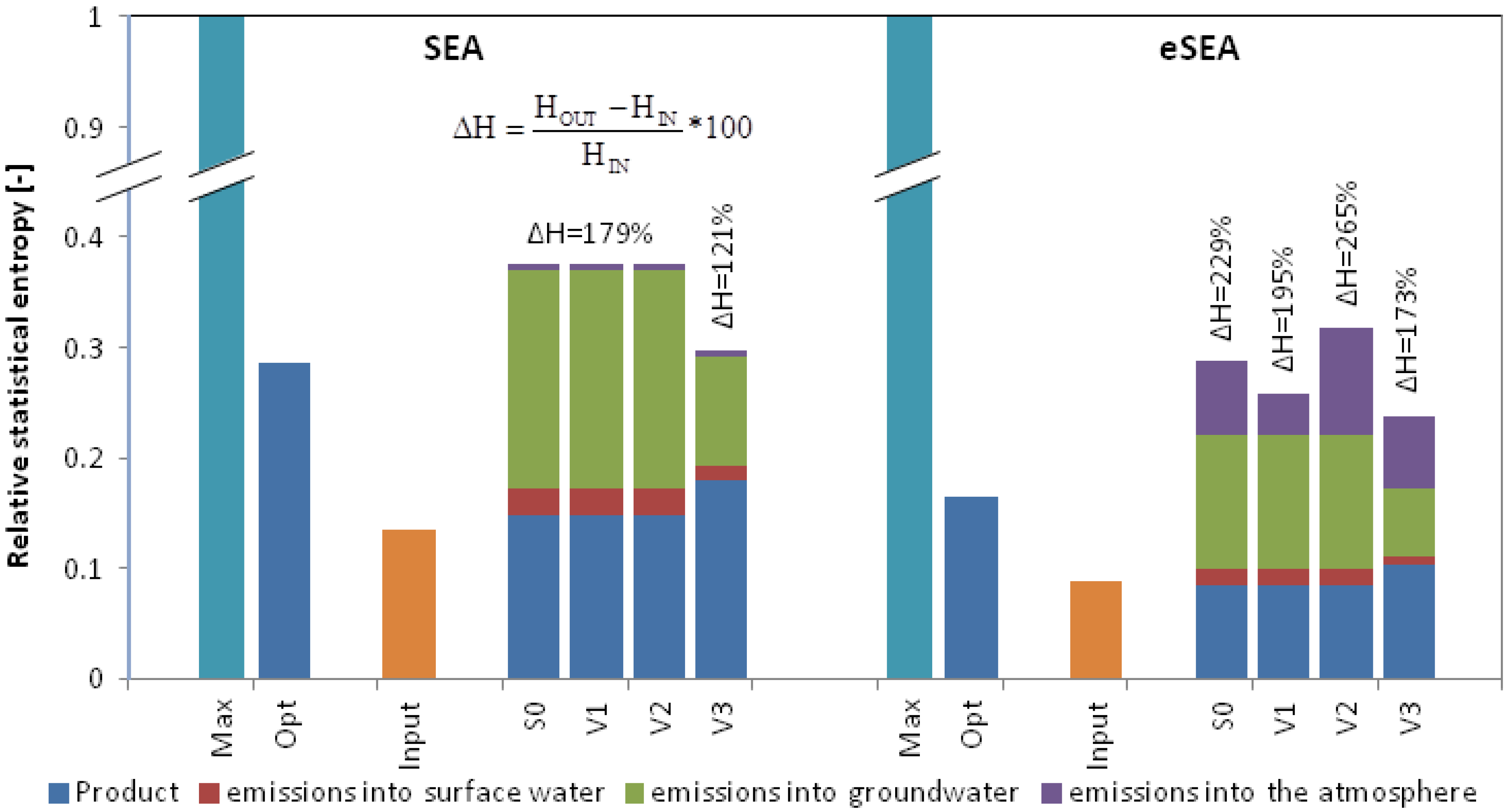
Figure 5. Relative statistical entropy values for the input and output of the base system (S0) and all variations (V1–V3) according to SEA and eSEA for the hypothetical crop farming region; entropy values are divided into entropy contributions from product yield and losses to the atmosphere, surface water, and groundwater.

Figure 5. Relative statistical entropy values for the input and output of the base system (S0) and all variations (V1–V3) according to SEA and eSEA for the hypothetical crop farming region; entropy values are divided into entropy contributions from product yield and losses to the atmosphere, surface water, and groundwater.

Both the SEA and eSEA confirm that nitrogen is diluted through the crop farming region (ΔH > 0). This is the case because the nitrogen in the fertilizer is more concentrated than that in the product: a typical result for a system where products are consumed or used. For both methods, the dilution lies in the range between the theoretical optimum and the theoretical worst case scenario (H_rel = 1). Note that the entropy results for the theoretical optimum are different for the SEA (H_opt,rel = 0.25) and eSEA (H_opt,rel = 0.16). This is due to the different input entropy values because, in contrast to the eSEA, the individual nitrogen compounds are not differentiated in SEA. In general, the SEA shows more preferential results (lower ΔH, less dilution) for systems S0–V3. However, neither a 50% reduction in gaseous emissions according to scenario V1 nor a 50% emission increase as described in scenario V2 are rewarded by the SEA because the total gaseous nitrogen emission does not change. Scenario V1 is clearly preferable due to its lower emissions of NH₃, N₂O and NO_x. The eSEA accounts for this result by calculating a lower extent of dilution (ΔH = 195%) in comparison to the original state (ΔH = 229%). Variation V2 is assessed with a higher ΔH of 265%. Lower ΔH values are obtained from both SEA and eSEA if emissions into the hydrosphere (surface and groundwater) are each decreased by 50% (V3). The SEA achieves a significantly better result for V3 (ΔH = 121%) than the eSEA (ΔH = 173%) because the SEA calculates the entropy generation from the sum of nitrogen being released into surface and groundwater while referring to a single corresponding nitrogen background concentration. On the other hand, the eSEA quantifies the entropy contribution from each nitrogen compound that is emitted into the hydrosphere with respect to the different corresponding background concentrations.

4. Application of the eSEA: A Numerical Example

In this section, a calculation for the system S0 (cf. Figure 3a) is given. Table 4a shows all relevant data along with intermediate results. Table 4b displays the final results.

Table 4. (a) Intermediate results for the eSEA on nitrogen compounds in the hypothetical crop farming region based on Austrian data (data rounded) and base system S0.

					(9)	(10)	(11)	(12,13)
		${\dot{\mathrm{M}}}_{\text{i}}$	cim	cim,geog	${\dot{\mathrm{X}}}_{\text{im}}$	mi	Xim	∑Xim
		kg/ha/yr	kgN/kg	kgN/kg	kgN/a	kg/kgN	kgN/kgN	kgN/kgN
INPUT	Fertilizer	211				4.74		1
	NH4NO3		0.13		28.20		0.63
	CO(NH2)2		0.01		1.80		0.04
	Seeds	25				0.56
	Norg		0.02		0.50		0.01
	Deposition	571				12.84
	NO3−		0.01		4.80		0.11
	NH4+		0.01		3.20		0.07
	N-fixation	8	0.76		6.00	0.18	0.13
OUTPUT	Product	2300				51.68		1
	Norg		0.01		23.00		0.52
	Off-gas	11				0.24
	N2		0.7553	0.7553	8.19		0.18
	NH3		0.16	4.1 E-9	1.75		0.04
	N2O		0.14	2.0 E-8	1.50		0.03
	NOx		0.02	2.5 E-10	0.20		4.5 E-03
	Surface water	42				0.94
	NO3−		2.0 E-02	3.0 E-06	0.85		0.02
	NH4+		2.4 E-03	1.2 E-06	0.10		2.3 E-03
	Norg		1.2 E-03	1.0 E-10	0.05		1.1 E-03
	Groundwater	373				8.37
	NO3−		2.0 E-02	1.0 E-05	7.52		0.17
	NH4+		2.4 E-03	3.5 E-07	0.90		0.02
	Norg		1.2 E-03	7.0 E-11	0.45		0.01

Table 4. (a) Intermediate results for the eSEA on nitrogen compounds in the hypothetical crop farming region based on Austrian data (data rounded) and base system S0.

					(9)	(10)	(11)	(12,13)
		${\dot{\mathrm{M}}}_{\text{i}}$	cim	cim,geog	${\dot{\mathrm{X}}}_{\text{im}}$	mi	Xim	∑Xim
		kg/ha/yr	kgN/kg	kgN/kg	kgN/a	kg/kgN	kgN/kgN	kgN/kgN
INPUT	Fertilizer	211				4.74		1
	NH4NO3		0.13		28.20		0.63
	CO(NH2)2		0.01		1.80		0.04
	Seeds	25				0.56
	Norg		0.02		0.50		0.01
	Deposition	571				12.84
	NO3−		0.01		4.80		0.11
	NH4+		0.01		3.20		0.07
	N-fixation	8	0.76		6.00	0.18	0.13
OUTPUT	Product	2300				51.68		1
	Norg		0.01		23.00		0.52
	Off-gas	11				0.24
	N2		0.7553	0.7553	8.19		0.18
	NH3		0.16	4.1 E-9	1.75		0.04
	N2O		0.14	2.0 E-8	1.50		0.03
	NOx		0.02	2.5 E-10	0.20		4.5 E-03
	Surface water	42				0.94
	NO3−		2.0 E-02	3.0 E-06	0.85		0.02
	NH4+		2.4 E-03	1.2 E-06	0.10		2.3 E-03
	Norg		1.2 E-03	1.0 E-10	0.05		1.1 E-03
	Groundwater	373				8.37
	NO3−		2.0 E-02	1.0 E-05	7.52		0.17
	NH4+		2.4 E-03	3.5 E-07	0.90		0.02
	Norg		1.2 E-03	7.0 E-11	0.45		0.01

Table 4. (b) Final results for the eSEA on nitrogen compounds in the hypothetical crop farming region based on Austrian data (data rounded) and base system S0.

		(19)	(21)	(15), (17)		(23)	(24)
		m'im	c'im	HIN / HOUT	HIN,rel / HOUT,rel	Hmax	ΔH
		[-]	[-]	[-]	[-]	[-]	[%]
INPUT	Fertilizer			3.52	0.09	40.38	229
	NH4NO3
	CO(NH2)2
	Seeds
	Norg
	Deposition
	NO3-
	NH4+
	N-fixation
OUTPUT	Product			11.60	0.29
	Norg
	Off-gas
	N2	2.4 E-01	7.553 E-01
	NH3	9.6 E+08	4.1 E-11
	N2O	1.7 E+08	2.0 E-10
	NOx	1.8 E+08	2.0 E-12
	Surface water
	NO3−	6.4 E+05	3.0 E-08
	NH4+	1.9 E+05	1.2 E-08
	Norg	1.1 E+09	1.0 E-12
	Groundwater
	NO3−	1.7 E+06	1.0 E-07
	NH4+	5.8 E+06	3.5 E-09
	Norg	1.4 E+10	7.0 E-13

Table 4. (b) Final results for the eSEA on nitrogen compounds in the hypothetical crop farming region based on Austrian data (data rounded) and base system S0.

		(19)	(21)	(15), (17)		(23)	(24)
		m'im	c'im	HIN / HOUT	HIN,rel / HOUT,rel	Hmax	ΔH
		[-]	[-]	[-]	[-]	[-]	[%]
INPUT	Fertilizer			3.52	0.09	40.38	229
	NH4NO3
	CO(NH2)2
	Seeds
	Norg
	Deposition
	NO3-
	NH4+
	N-fixation
OUTPUT	Product			11.60	0.29
	Norg
	Off-gas
	N2	2.4 E-01	7.553 E-01
	NH3	9.6 E+08	4.1 E-11
	N2O	1.7 E+08	2.0 E-10
	NOx	1.8 E+08	2.0 E-12
	Surface water
	NO3−	6.4 E+05	3.0 E-08
	NH4+	1.9 E+05	1.2 E-08
	Norg	1.1 E+09	1.0 E-12
	Groundwater
	NO3−	1.7 E+06	1.0 E-07
	NH4+	5.8 E+06	3.5 E-09
	Norg	1.4 E+10	7.0 E-13

5. Conclusions

This paper presents an evaluation method based on statistical entropy (eSEA) for assessing the concentration and dilution of chemical compounds in a system. It demonstrates how the eSEA can be applied to assess the nitrogen performance of a hypothetical crop farming region based on data from Austria. The results show that the optimal utilization of nitrogen (maximum yield) occurs with low entropy production and that significant losses of nitrogen to the environment produce entropy. Therefore, eSEA may have the potential to become a meaningful indicator for the quality of regional substance management. In our ongoing work, we will apply eSEA to real (and more complex) Austrian regions to test its relevance for decision-making in regional nutrient management.