Control Parameters for Boundary-Layer Instabilities in Unsteady Shock Interactions

Abstract

This article presents the computation of a set of control parameters for the deterministic prediction of laminar boundary-layer instabilities induced by an imposed unsteady shock interaction. The objective of the study is exploratory in nature by computing a supersonic flight environment for flow over a blunt body and the deterministic prediction of the spectral entropy rates for the boundary layer subjected to an unsteady pressure disturbance. The deterministic values for the spectral entropy rate within the instabilities are determined for each control parameter. Computational results imply that the instabilities are of a span-wise vortex form, that the maximum vertical velocity wave vector components are produced in the region nearest the wall and that extended transient coherent structures are produced in the boundary layer at a vertical location slightly below the mid-point of the boundary layer.

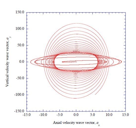
1. Introduction

Considerable progress has been made in understanding the role that different values of the control parameters play in determining the computational output from nonlinear deterministic equations. Klimontovich and Bonitz [1] studied the self-organization process resulting from two control parameters. Kapitaniak [2] presents a discussion of the various feedback parameters in controlling chaos. [2] also presents reprints of thirteen important contributions to the study of the effects of parameter values on controlling chaos. Two papers by Pyragas [3,4] are of particular interest in our study of the effects of control parameters on the prediction of instabilities arising in boundary layers subjected to external disturbances. In these two papers, Pyragas discusses the roles of both internal and external feedback control parameters in providing continuous control of chaotic behavior.

In the approach that we describe here, a set of coupled, nonlinear deterministic equations for fluctuating velocity wave vectors (see [5]) is embedded in the Falkner-Skan boundary-layer profiles calculated in both the axial-vertical velocity plane and the span wise-vertical velocity plane. This approach requires three internal control parameters and two externally applied control parameters.

The first internal control parameter is the set of mean velocity gradients computed in the boundary layer profiles in both the axial velocity plane and the span wise velocity plane. These gradients are evaluated at each vertical station in the respective velocity profiles and serve as input for the required coefficients in the coupled, nonlinear deterministic equations. The coupled, nonlinear deterministic equations are solved for selected vertical stations within the boundary layers, with the resulting nonlinear time series serving as the source for the analysis of possible boundary-layer instabilities.

The second internal control parameter consists of the span wise location of the determination of the velocity gradients in the span-wise, vertical velocity plane. The third internal control parameter is a weighted, linearization factor determining the degree of coupled nonlinearity incorporated within the set of deterministic equations.

The externally imposed unsteady pressure disturbance provides two additional feedback control parameters. These are, first, the frequency factor for the unsteady imposed wave, and, second, the amplification factor for the wave.

The environment for the analysis of this computational approach consists of the supersonic to hypersonic flow of air around a flight vehicle that produces an upstream oblique shock wave that intersects a down stream detached bow shock wave. The model configuration for this flow is the spiked-blunt body flow field, consisting of an attached conical oblique shock wave that impinges on the detached bow shock wave of the blunt body surface. Panaras and Drikakis [6] have presented a recent review of the progress made in understanding the unsteady flow around spiked-blunt bodies in high-speed flow. Drikakis and Rider [7] present the computational tools used in the mathematical modeling of these flows.

For hypersonic propulsion flight vehicles, the inlet to the propulsion system may consist of a rectangular shape, with an upper plate forward of the lower, engine inlet cowl. In this supersonic flow environment, a bow shock wave is produced forward of the lower engine cowl. An oblique shock wave, produced by the upper plate, impinges on the lower detached bow shock wave. Lind and Lewis [8] and Lind [9] have numerically mapped the resulting flow field and demonstrated the production of an imposed pressure disturbance on the engine cowl boundary layer.

The first section in this paper determines the thermodynamic and transport properties for this flow environment at a selected flight Mach number and flight altitude. These properties determine the kinematic viscosity used in the boundary layer calculations.

The second section of the paper presents the computational basis for the evaluation of the axial-vertical plane velocity gradients and the span wise-vertical velocity gradients. To facilitate the utilization of appropriate boundary layer results for the computation of boundary layer instabilities, we have included tables of the appropriate velocity gradients for each of the boundary layer velocity profiles.

A modified form [5] of the flow equations developed by Townsend [10], describing the fluctuating velocity components, is presented in the third section. The integration in time of these coupled, nonlinear deterministic equations, with the incorporation of the various control parameters, yields the nonlinear time series output for each of the respective fluctuating velocity wave vectors.

The fourth section of the paper discusses Burg’s method [11,12] for the extraction of the power spectral density of the sum of the squares of the axial and vertical velocity wave vectors from the nonlinear time series data. A key part of the paper is presented is this section to clarify the differences between Burg’s method for the extraction of the power spectral density from nonlinear time series data, and the determination of the spectral entropy rate characteristics which are inherent within the power spectral density data sets. It is especially important to draw attention to the meaning of the phase “spectral entropy rate pulses” as it is used in this paper.

The spectral entropy rate [13] is described as a concept to distinguish “regular” from “irregular” trajectories as predicted in the solution of nonlinear deterministic differential equations. We employ the concept of the spectral entropy rate to identify “coherent’ structures within the power spectral density time series from “chaotic” structures within the same time series data. Thus, when we discuss the “spectral entropy rate pulse”, we are using the phase to describe whether the computed power spectral density time series is in a conceptual “chaotic structure” mode (high values of the spectral entropy rate approaching the value of 0.345 1/s for possible chaotic behavior) or whether it is in a “coherent structure” mode (low values of the spectral entropy rate, approaching the value of 0.0 for possible span wise periodic vortex structures).

Putting all of this together, we are in a position to examine the effects of each of the control parameters on the production of “coherent” or “chaotic” structures at various locations in the vertical velocity profiles as a function of the time integration of the coupled, nonlinear deterministic modified Townsend equations.

The results of these computations are presented in a series of graphs representing the behavior of the spectral entropy rate pulses for a set of values for each of the respective control parameters. It is observed that for the prediction of the presence of boundary layer instabilities, velocity gradients of the span wise-vertical velocity profiles must be included in the internal set of control parameters. Further, the span wise location for the evaluation of the span wise vertical velocity gradients has a direct bearing on the prediction of the rate of production of the pulses in the spectral entropy content of the time series. Additional observations are presented in the discussion of the results.

From the computational results, we may observe first, that for the imposed pressure disturbances, significant vertical velocity wave vector fluctuations occur in the region next to the wall beneath the imposed pressure disturbance. This has significant implications for the evaluation of wall heat transfer at higher flight Mach numbers. Second, significant “coherent” structures (vortices?) occur within the boundary layer just below the mid-point of the normalized vertical thickness of the boundary layer.

2. Supersonic Flight Environment

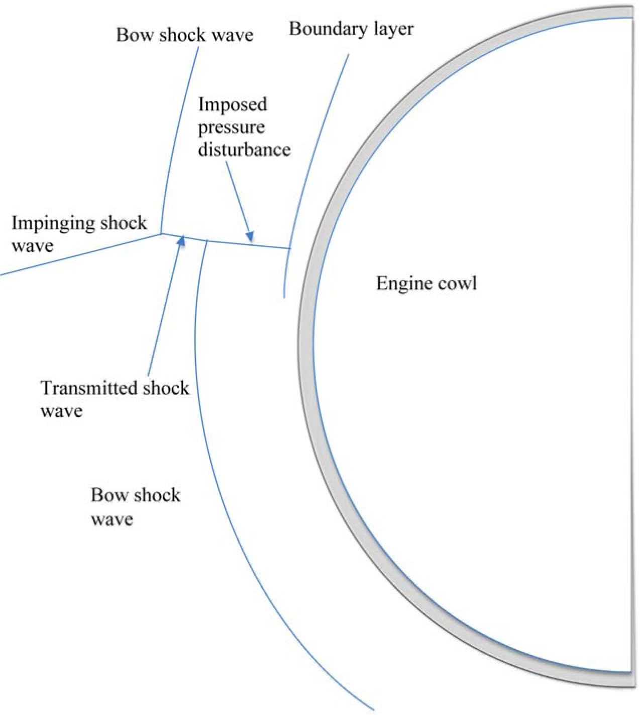
Considerable progress has been made in the development of hypersonic flight propulsion. Present configurations of hypersonic propulsion systems include an engine-integrated airframe in which the forebody acts as the engine compression surface and the afterbody serves as the engine nozzle [14,15]. [8,9] report the results of extensive numerical evaluations of the interactions of the inlet oblique shock wave with the bow shock wave produced by the engine cowl. The flow configuration that we are approximating in this exploratory study is shown in Figure 1, modeled after Figure 9 of [9]. In this approximate flow environment, the oblique shock wave from the forward inlet structure impinges on the engine cowl bow shock wave. This shock wave interaction results in a transmitted shock wave and an imposed pressure disturbance acting on the subsonic boundary layer formed over the surface of the engine cowl structure. The results presented in [9] indicate that this imposed pressure disturbance may be unsteady in nature. Our objectives here are to explore a possible mechanism for the time-dependent formation of vortex-like coherent structures within the boundary layer and to present a set of control parameters which yield the numerical results predicting such transient ordered structures.

The flight conditions considered in this study are a modest flight Mach number of M₁ = 1.44 at an altitude of approximately 21,300 m. For these conditions, the atmospheric temperature is taken as t₁ = 217.76 K and the atmospheric pressure is p₁ = 4.54 × 10³ N/m² [16]. At this altitude, flight Mach numbers between 1.44 and 2.50 yield static temperatures behind the bow shock wave between 279.1 K and 458.7 K. In this range of temperatures, the ratio of specific heats for air is essentially constant at 1.40. As the flight Mach number increases beyond 2.50, variation in the thermodynamic properties of the air behind the bow shock wave will need to be taken into account.

Figure 1. Two-dimensional supersonic flow indicating an impingement shock wave on the bow shock wave of an engine cowl. Note the development of an imposed pressure disturbance on the cowl boundary layer.

Figure 1. Two-dimensional supersonic flow indicating an impingement shock wave on the bow shock wave of an engine cowl. Note the development of an imposed pressure disturbance on the cowl boundary layer.

The thermodynamic properties that are required for the calculation of the boundary layer development are obtained from standard gas dynamic relations for normal shock waves [17]. The Mach number immediately downstream of the normal bow shock wave ahead of the engine cowl is given by:

$$M_2^2=\frac{M_1^2+\frac{2}{\gamma +1}}{\frac{2\gamma }{\gamma -1}{M}_1^2-1}$$

(1)

In this expression, M₁ is the upstream Mach number, M₂ is the shock wave downstream Mach number, and γ is the ratio of specific heats for air at these conditions. For the flight conditions given, the downstream Mach number is M₂ = 0.723, the static temperature is t₂ = 278.88 K, and the static pressure is p₂ = 1.019154 × 10⁴ N/m².

The thermodynamic and transport properties, required for the determination of the effects of the control parameters, are sensitive to the choice of temperature and pressure values for their evaluation. For example, the kinematic viscosity of the air is required for the evaluation of the boundary-layer velocity gradients. This parameter is dependent upon both the temperature and the pressure of the air in the boundary layer environment. Assuming that the surface of the blunt body is insulated, the adiabatic wall temperature and the static pressure behind the bow shock wave are used as the reference thermodynamic conditions for the evaluation of this parameter. The adiabatic wall temperature, T_aw, is define as [18]:

$$T_{aw}=t_2[1+R_c\frac{\gamma -1}{2}{M}_2^2]$$

(2)

In this expression, R_c is the recovery factor, which is closely determined by the rule:

$$R_c=\sqrt{{\mathrm{Pr}}_f}$$

(3)

where Pr_f is the Prandtl number for the flowing gas mixture. The Prandtl number, Pr_f, is defined by the equation:

$${\mathrm{Pr}}_f=\frac{C_{pf}{\mu }_f}{{\kappa }_f}$$

(4)

The specific heat at constant pressure, C_pf is the specific heat of the mixture of the molecular species making up the gas, μ_f is the dynamic viscosity of the gas mixture, and κ_f is the thermal conductivity of the gas mixture.

Since the various properties in the Prandtl number are temperature dependent, an iterative solution is required to determine the appropriate value of the adiabatic wall temperature. A mixture of 0.002% CO₂, 0.002% H₂O, 21.052% O₂, and 78.944% N₂, with percent by volume, was used as the working gas. Empirical expressions for the specific heats of the various components were obtained from Heywood [19], corresponding expressions for the dynamic viscosity of the components were obtained from [20], and the thermal conductivity expressions were obtained by polynomial fit to the data presented by Mills [21].

The thermodynamic and transport properties for mixtures of polyatomic gases are determined by the procedures presented by Dorrance [22]. It should be noted that as flight Mach numbers increase into the hypersonic range, the gas temperatures become sufficiently high that variations of these properties must be taken into account. Also, active methods of cooling the surface may be necessary, such as the transpiration of hydrogen, H₂ into the boundary layer. Gas mixtures, such as H₂ into air (O₂ and N₂), produce mixture Prandtl numbers significantly lower than those predicted for polyatomic gas mixtures. This effect will change the value of the adiabatic wall temperature used in the calculation of the kinematic viscosity, which is the primary transport property used in the calculation of the effects of the control parameters on the boundary-layer instabilities.

The results for the various thermodynamic and transport properties for the flight Mach number of M₁ = 1.44 at an altitude of 21.3 km are as follows:

Adiabatic wall temperature, T_aw; 303.64 K

(5)

Static pressure, p₂: 1.019154 × 10⁴ N/m²

(6)

Mixture Prandtl number, Pr_f: 0.7101

(7)

The kinematic viscosity for air has been calculated using an expression from [20] for the dynamic viscosity of air as a function of temperature. For the resulting adiabatic wall temperature and the given static pressure behind the shock wave, the kinematic viscosity for air is determined to be:

Air kinematic viscosity, ν: 1.599 × 10⁻⁴ m²/s

(8)

This value for the kinematic viscosity for air is used for the evaluation of the various boundary layer velocity gradients and for the prediction of boundary layer instabilities

3. Boundary-Layer Flow Environment

The basic objective of this study is to use the boundary layer flow environments computed with well-established computational tools to establish a basis for the determination of a set of spectral entropy rate production values calculated at an upstream location of a laminar boundary layer flow subjected to an externally imposed pressure disturbance. Cebeci and Bradshaw [23] have developed a set of computer source codes for the computation of various wall shear environments. These source codes have been used to create computer programs required to compute the desired boundary layer flows, including the necessary gradients in the mean velocities in a three-dimensional configuration.

3.1. Computational Model for the Boundary-Layer Flow

The flow configuration we wish to model is the three-dimensional wall shear layer downstream of an initial starting plane, as indicated in Figure 2. The flow is from left to right and is assumed to be an ideal gas moving at subsonic velocity over a flat plate with laminar flow.

The computational procedure developed in [23] is used as the basis for our computations of the boundary layer flow. The flow is of the Falkner-Skan type with an adverse pressure gradient in the axial direction only. The modification, which we introduce, is to impose an initial free stream velocity of unity, making the boundary layer edge velocity dimensionless. The main computer program in the computational procedure developed in [23] establishes “nx” as the station number for the axial direction and the symbol “j” for the vertical grid number for the calculation of the vertical profiles at a given axial station. Following the nomenclature used in the computer program development, we will use “nx” throughout this article to identify the axial station calculations and the vertical grid number “j” to specify the values of the appropriate vertical parameters. We also will include the corresponding axial distance with the nx value and the corresponding η value with the vertical station number j.

Figure 2. The three-dimensional flow model and the coordinate system for the boundary layer flow environment. Note the location for the laminar flow velocity profile computations.

Figure 2. The three-dimensional flow model and the coordinate system for the boundary layer flow environment. Note the location for the laminar flow velocity profile computations.

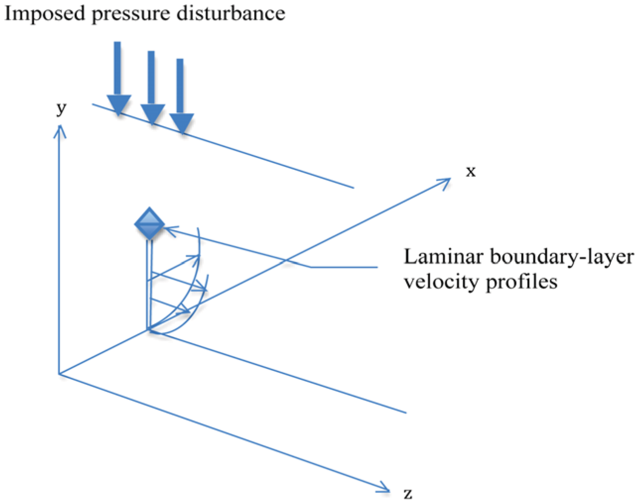
In an analysis of the conditions for similarity in boundary layer flows, Hansen [24] indicates that both the Blasius profile of the axial velocity in the x-y plane and the Blasius profile in the z-y plane along the original starting planes are similar. Hence, we apply the computer methods of [23] to the computation of the laminar velocity profile in the x-y plane at the axial station, nx = 4 (x = 0.08), along the x-axis, and the same computer methods to the computation of the laminar velocity profile in the z-y plane at the span wise station, nz = 4 (z = 0.003), along the z-axis, with no pressure gradient in the z direction.

The implementation of the calculations for the effect of the control parameters within the boundary-layer flow requires the evaluation of velocity gradients in a three-dimensional format. We have again followed the procedure of [23] in implementing a computational procedure for the development of the boundary layer along the z-y plane as indicated in Figure 2. Here, however, we uncouple the x-y plane boundary-layer development from the z-y plane and apply the same computer procedure as outlined above to the flow along the z-y plane at the initial laminar region of nx = 4 (x = 0.08), where nx is the axial station number for the development of the initial laminar flow in the axial direction and nz = 4 as the corresponding location in the z-direction. This procedure thus yields the necessary velocity gradients in the z-y plane for the computation of the unsteady velocity fluctuations in the unstable region of the boundary-layer flow. Since the mathematical and computational procedures for the computation of the boundary layer flow are fully developed and described in [23], only an outline of the boundary-layer computational procedure is presented here. Where we have used expressions for mean velocity gradients that do not appear in these references, we provide more detail. The momentum equations for the boundary-layer flow may be written as:

$$u\frac{\partial u}{\partial x}+v\frac{\partial u}{\partial y}=-\frac{1}{\rho }\frac{dp}{dx}+\frac{1}{\rho }\frac{\partial }{\partial y}\left[\mu \frac{\partial u}{\partial y}\right]$$

(9)

(the meaning of each of the symbols is given in the Nomenclature).

The boundary conditions are:

$$y=0, u=v=0$$

(10)

$$y=\delta (x), u=u_e\left(x\right)$$

(11)

Following [23], the Falkner-Skan transformation is defined by:

$$\eta ={\left(\frac{u_e}{\nu x}\right)}^{1/2}y$$

(12)

The velocity at the edge of the boundary layer, $u_e=u_e\left(x\right)$, is assumed to vary with distance x. A dimensionless stream function, $f(x,\eta )$, is introduced and is given by:

$$\Psi (x,y)={\left(u_e\nu x\right)}^{1/2}f(x,\eta )$$

(13)

These definitions yield the results for velocities u and v as [23]:

$$u=u_e{f}^{\prime }, v=-\frac{\partial }{\partial }\frac{}{x}[(u_e\nu {x)}^{1/2}f]+\frac{\eta }{2}{\left(\frac{u_e\nu }{x}\right)}^{1/2}{f}^{\prime }$$

(14)

In these expressions, the prime indicates differentiation with respect to $\eta$.

The velocity gradients in both the x-y plane and the z-y plane are required for the evaluation of instabilities produced within the boundary layer by the imposed pressure disturbances. These values thus form the first set of internal control parameters. The set of velocity gradients required are the following:

$$\frac{\partial u}{\partial x}\frac{\partial u}{\partial y}\frac{\partial u}{\partial z}$$

(15)

$$\frac{\partial v}{\partial x}\frac{\partial v}{\partial y}\frac{\partial v}{\partial z}$$

(16)

$$\frac{\partial w}{\partial x}\frac{\partial w}{\partial y}\frac{\partial w}{\partial z}$$

(17)

With the assumption that the velocity profiles in the z-y plane are independent of the profiles in the x-y plane, we may write:

$$\frac{\partial u}{\partial z}=\frac{\partial w}{\partial x}=0$$

(18)

From the continuity equations in both the x-y plane and in the z-y plane, we may write:

$$\frac{\partial v}{\partial y}=-\frac{\partial u}{\partial x};\frac{\partial w}{\partial y}=-\frac{\partial v}{\partial z}$$

(19)

Utilizing the transformed variables from [23], the appropriate velocity gradients are obtained from the computational output with the following equations [5]:

$$\frac{\partial u}{\partial x}=-f^{″}\left(\frac{u}{x}\right)\left(\frac{\eta }{2}\right)$$

(20)

$$\frac{\partial u}{\partial y}=f^{″}\frac{u}{x}\sqrt{\frac{ux}{\nu }}$$

(21)

$$\frac{\partial v}{\partial x}=-\frac{1}{4}\left(\frac{u}{x}\right)\frac{1}{\sqrt{\frac{ux}{\nu }}}[{\eta }^2{f}^{″}+\left(\eta f^{\prime }-f\right)]$$

(22)

$$\frac{\partial v}{\partial y}=f^{″}\left(\frac{u}{x}\right)\left(\frac{\eta }{2}\right)$$

(23)

In these expressions, the prime indicates differentiation with respect to η. Corresponding expressions are used to determine similar velocity gradients in the z-y plane.

The flow conditions that correspond to a kinematic viscosity of 1.599 × 10⁻⁴ m²/s are an adiabatic wall temperature T_aw = 303.64 K and a boundary layer edge pressure p₂ = 10191.54 N/m². These values are considered applicable as the flow temperature and pressure for the boundary layer and are used for the boundary layer calculations. The density is calculated from the ideal gas equation of state and the dynamic viscosity for air is calculated from the expression given in [20].

We assume for convenience that the basic flow environment corresponds to a flow with the boundary-layer edge velocity given by:

$$u_e=\left(1-\frac{x}{8}\right)$$

(24)

In this expression, u_e is the dimensionless boundary layer edge velocity and x is the dimensionless axial distance. The corresponding dimensionless pressure gradient parameter, m, is given by:

$$m=\left(\frac{x}{u_e}\right)\left(\frac{-1}{8}\right)$$

(25)

The velocity profiles are obtained from the computational procedure at nx = 4 (x = 0.08), thus initially computing the boundary layer as laminar. The length and width of the plate are each taken as 1.0 m.

For the flow in the z direction, we take the external velocity w_e = 0.01, with a pressure gradient of zero in the z direction. The z-y plane laminar velocity gradients are obtained at a span wise station of nz = 4 (z = 0.003), at the axial station of nx = 4 (x = 0.08). This procedure allows us to estimate the required velocity gradients in the initially laminar region in a three-dimensional configuration, as indicated in Figure 2.

The computational results for the velocity gradients in the x-y plane are presented in Table 1. The corresponding velocity gradients in the z-y plane are presented in Table 2. These values for the velocity gradients form the first set of internal control parameters required for the solution of the modified Townsend equations. The values presented in these tables allow the computation of the boundary-layer instabilities independently of boundary-layer computations.

Table 1. Boundary-layer x-y plane velocity gradients. Kinematic viscosity, ν = 1.599 × 10⁻⁴ m²/s, x = 0.08.

j	η	$\partial U/\partial x$	$\partial U/\partial y$	$\partial V/\partial x$	$\partial V/\partial y$
1	0.0000
2	0.2000	−0.3953	87.9648	0.0018	0.3953
3	0.4000	−0.7921	88.1166	0.0098	0.7921
4	0.6000	−1.1855	87.9006	0.0231	1.1855
5	0.8010	−1.5686	87.2045	0.0415	1.5686
6	1.0010	−1.9325	85.9288	0.0647	1.9325
7	1.2020	−2.2673	83.9931	0.0919	2.2673
8	1.4020	−2.5624	81.3431	0.1223	2.5624
9	1.6030	−2.8073	77.9565	0.1548	2.8073
10	1.8040	−2.9925	73.8486	0.1881	2.9925
11	2.0050	−3.1108	69.0742	0.2207	3.1108
12	2.2060	−3.1578	63.7273	0.2512	3.1578
13	2.4070	−3.1326	57.9367	0.2784	3.1326
14	2.6080	−3.0384	51.8577	0.3010	3.0384
15	2.8090	−2.8818	45.6616	0.3183	2.8818
16	3.0110	−2.6733	39.5230	0.3298	2.6733
17	3.2120	−2.4252	33.6067	0.3356	2.4252
18	3.4140	−2.1518	28.0563	0.3360	2.1518
19	3.6150	−1.8670	22.9850	0.3317	1.8670
20	3.8170	−1.5841	18.4706	0.3238	1.5841
21	4.0190	−1.3142	14.5540	0.3132	1.3142
22	4.2210	−1.0661	11.2411	0.3010	1.0661
23	4.4230	−0.8455	8.5083	0.2883	0.8455
24	4.6250	−0.6557	6.3093	0.2758	0.6557
25	4.8280	−0.4971	4.5829	0.2642	0.4971
26	5.0300	−0.3685	3.2603	0.2539	0.3685
27	5.2330	−0.2670	2.2711	0.2451	0.2670
28	5.4350	−0.1891	1.5489	0.2378	0.1891
29	5.6380	−0.1310	1.0341	0.2320	0.1310
30	5.8410	−0.0887	0.6757	0.2275	0.0887
31	6.0440	−0.0587	0.4321	0.2242	0.0587
32	6.2470	−0.0380	0.2704	0.2218	0.0380
33	6.4500	−0.0240	0.1656	0.2200	0.0240
34	6.6530	−0.0148	0.0992	0.2188	0.0148
35	6.8560	−0.0090	0.0581	0.2180	0.0090
36	7.0600	−0.0053	0.0333	0.2175	0.0053
37	7.2630	−0.0030	0.0187	0.2172	0.0030
38	7.4670	−0.0017	0.0102	0.2170	0.0017
39	7.6710	−0.0009	0.0055	0.2168	0.0009
40	7.8750	−0.0005	0.0029	0.2168	0.0005
41	8.0780	0.0000	0.0000	0.0000	0.0000

Table 1. Boundary-layer x-y plane velocity gradients. Kinematic viscosity, ν = 1.599 × 10⁻⁴ m²/s, x = 0.08.

j	η	$\partial U/\partial x$	$\partial U/\partial y$	$\partial V/\partial x$	$\partial V/\partial y$
1	0.0000
2	0.2000	−0.3953	87.9648	0.0018	0.3953
3	0.4000	−0.7921	88.1166	0.0098	0.7921
4	0.6000	−1.1855	87.9006	0.0231	1.1855
5	0.8010	−1.5686	87.2045	0.0415	1.5686
6	1.0010	−1.9325	85.9288	0.0647	1.9325
7	1.2020	−2.2673	83.9931	0.0919	2.2673
8	1.4020	−2.5624	81.3431	0.1223	2.5624
9	1.6030	−2.8073	77.9565	0.1548	2.8073
10	1.8040	−2.9925	73.8486	0.1881	2.9925
11	2.0050	−3.1108	69.0742	0.2207	3.1108
12	2.2060	−3.1578	63.7273	0.2512	3.1578
13	2.4070	−3.1326	57.9367	0.2784	3.1326
14	2.6080	−3.0384	51.8577	0.3010	3.0384
15	2.8090	−2.8818	45.6616	0.3183	2.8818
16	3.0110	−2.6733	39.5230	0.3298	2.6733
17	3.2120	−2.4252	33.6067	0.3356	2.4252
18	3.4140	−2.1518	28.0563	0.3360	2.1518
19	3.6150	−1.8670	22.9850	0.3317	1.8670
20	3.8170	−1.5841	18.4706	0.3238	1.5841
21	4.0190	−1.3142	14.5540	0.3132	1.3142
22	4.2210	−1.0661	11.2411	0.3010	1.0661
23	4.4230	−0.8455	8.5083	0.2883	0.8455
24	4.6250	−0.6557	6.3093	0.2758	0.6557
25	4.8280	−0.4971	4.5829	0.2642	0.4971
26	5.0300	−0.3685	3.2603	0.2539	0.3685
27	5.2330	−0.2670	2.2711	0.2451	0.2670
28	5.4350	−0.1891	1.5489	0.2378	0.1891
29	5.6380	−0.1310	1.0341	0.2320	0.1310
30	5.8410	−0.0887	0.6757	0.2275	0.0887
31	6.0440	−0.0587	0.4321	0.2242	0.0587
32	6.2470	−0.0380	0.2704	0.2218	0.0380
33	6.4500	−0.0240	0.1656	0.2200	0.0240
34	6.6530	−0.0148	0.0992	0.2188	0.0148
35	6.8560	−0.0090	0.0581	0.2180	0.0090
36	7.0600	−0.0053	0.0333	0.2175	0.0053
37	7.2630	−0.0030	0.0187	0.2172	0.0030
38	7.4670	−0.0017	0.0102	0.2170	0.0017
39	7.6710	−0.0009	0.0055	0.2168	0.0009
40	7.8750	−0.0005	0.0029	0.2168	0.0005
41	8.0780	0.0000	0.0000	0.0000	0.0000

Table 2. Boundary-layer z-y plane velocity gradients. Kinematic viscosity, ν = 1.599 × 10⁻⁴ m²/s, z = 0.003.

j	η	$\partial W/\partial z$	$\partial W/\partial y$	$\partial V_z/\partial z$	$\partial V_z/\partial y$
1	0.0000
2	0.2000	−2.2089	15.1271	−0.1613	2.2089
3	0.4000	−4.3987	15.0620	−0.6423	4.3987
4	0.6000	−6.5437	14.9379	−1.4333	6.5437
5	0.8000	−8.6074	14.7368	−2.5137	8.6074
6	1.0000	−10.5449	14.4432	−3.8494	10.5449
7	1.2000	−12.3050	14.0449	−5.3903	12.3050
8	1.4000	−13.8338	13.5342	−7.0700	13.8338
9	1.6000	−15.0793	12.9086	−8.8075	15.0793
10	1.8000	−15.9963	12.1721	−10.5110	15.9963
11	2.0000	−16.5510	11.3348	−12.0839	16.5510
12	2.2000	−16.7256	10.4130	−13.4325	16.7256
13	2.4000	−16.5210	9.4285	−14.4744	16.5210
14	2.6000	−15.9583	8.4068	−15.1465	15.9583
15	2.8000	−15.0779	7.3757	−15.4117	15.0779
16	3.0000	−13.9362	6.3627	−15.2622	13.9362
17	3.2000	−12.6013	5.3937	−14.7203	12.6013
18	3.4000	−11.1469	4.4905	−13.8352	11.1469
19	3.6000	−9.6461	3.6700	−12.6766	9.6461
20	3.8000	−8.1657	2.9433	−11.3274	8.1657
21	4.0000	−6.7621	2.3155	−9.8740	6.7621
22	4.2000	−5.4778	1.7864	−8.3986	5.4778
23	4.4000	−4.3408	1.3512	−6.9722	4.3408
24	4.6000	−3.3648	1.0019	−5.6503	3.3648
25	4.8000	−2.5515	0.7281	−4.4709	2.5515
26	5.0000	−1.8927	0.5185	−3.4547	1.8927
27	5.2000	−1.3735	0.3618	−2.6072	1.3735
28	5.4000	−0.9750	0.2473	−1.9220	0.9750
29	5.6000	−0.6771	0.1656	−1.3842	0.6771
30	5.8000	−0.4600	0.1086	−0.9739	0.4600
31	6.0000	−0.3057	0.0698	−0.6695	0.3057
32	6.2000	−0.1987	0.0439	−0.4497	0.1987
33	6.4000	−0.1263	0.0270	−0.2952	0.1263
34	6.6000	−0.0786	0.0163	−0.1894	0.0786
35	6.8000	−0.0478	0.0096	−0.1187	0.0478
36	7.0000	−0.0284	0.0056	−0.0727	0.0284
37	7.2000	−0.0165	0.0031	−0.0435	0.0165
38	7.4000	−0.0094	0.0017	−0.0254	0.0094
39	7.6000	−0.0052	0.0009	−0.0146	0.0052
40	7.8000	−0.0029	0.0005	−0.0081	0.0029
41	8.0000	0.0000	0.0000	0.0000	0.0000

Table 2. Boundary-layer z-y plane velocity gradients. Kinematic viscosity, ν = 1.599 × 10⁻⁴ m²/s, z = 0.003.

j	η	$\partial W/\partial z$	$\partial W/\partial y$	$\partial V_z/\partial z$	$\partial V_z/\partial y$
1	0.0000
2	0.2000	−2.2089	15.1271	−0.1613	2.2089
3	0.4000	−4.3987	15.0620	−0.6423	4.3987
4	0.6000	−6.5437	14.9379	−1.4333	6.5437
5	0.8000	−8.6074	14.7368	−2.5137	8.6074
6	1.0000	−10.5449	14.4432	−3.8494	10.5449
7	1.2000	−12.3050	14.0449	−5.3903	12.3050
8	1.4000	−13.8338	13.5342	−7.0700	13.8338
9	1.6000	−15.0793	12.9086	−8.8075	15.0793
10	1.8000	−15.9963	12.1721	−10.5110	15.9963
11	2.0000	−16.5510	11.3348	−12.0839	16.5510
12	2.2000	−16.7256	10.4130	−13.4325	16.7256
13	2.4000	−16.5210	9.4285	−14.4744	16.5210
14	2.6000	−15.9583	8.4068	−15.1465	15.9583
15	2.8000	−15.0779	7.3757	−15.4117	15.0779
16	3.0000	−13.9362	6.3627	−15.2622	13.9362
17	3.2000	−12.6013	5.3937	−14.7203	12.6013
18	3.4000	−11.1469	4.4905	−13.8352	11.1469
19	3.6000	−9.6461	3.6700	−12.6766	9.6461
20	3.8000	−8.1657	2.9433	−11.3274	8.1657
21	4.0000	−6.7621	2.3155	−9.8740	6.7621
22	4.2000	−5.4778	1.7864	−8.3986	5.4778
23	4.4000	−4.3408	1.3512	−6.9722	4.3408
24	4.6000	−3.3648	1.0019	−5.6503	3.3648
25	4.8000	−2.5515	0.7281	−4.4709	2.5515
26	5.0000	−1.8927	0.5185	−3.4547	1.8927
27	5.2000	−1.3735	0.3618	−2.6072	1.3735
28	5.4000	−0.9750	0.2473	−1.9220	0.9750
29	5.6000	−0.6771	0.1656	−1.3842	0.6771
30	5.8000	−0.4600	0.1086	−0.9739	0.4600
31	6.0000	−0.3057	0.0698	−0.6695	0.3057
32	6.2000	−0.1987	0.0439	−0.4497	0.1987
33	6.4000	−0.1263	0.0270	−0.2952	0.1263
34	6.6000	−0.0786	0.0163	−0.1894	0.0786
35	6.8000	−0.0478	0.0096	−0.1187	0.0478
36	7.0000	−0.0284	0.0056	−0.0727	0.0284
37	7.2000	−0.0165	0.0031	−0.0435	0.0165
38	7.4000	−0.0094	0.0017	−0.0254	0.0094
39	7.6000	−0.0052	0.0009	−0.0146	0.0052
40	7.8000	−0.0029	0.0005	−0.0081	0.0029
41	8.0000	0.0000	0.0000	0.0000	0.0000

4. Mathematical Model of the Flow Instability

4.1. Transformation of the Townsend Equations

Considerable effort has recently been devoted to the study of the transition of laminar boundary layers brought about by the existence of free-stream disturbances. Recent work has been presented in [25,26,27,28,29,30]. These references present an extensive review of the recent work in this field and hence a review of this work will not be repeated here. However, several aspects of the so-called by-pass transition process are essential to our mathematical model and hence will be discussed here. One of the essential aspects of these studies is the evidence that strong free-stream turbulence produces elongated stream wise structures with narrow span wise scales. These disturbances apparently give rise to a periodic modulation of the stream wise velocity. We will use the results of [25,26,27,28,29,30] to further investigate the possibilities of the existence of vertical bursts occurring near the wall in a boundary-layer flow.

The Navier-Stokes equations describing this flow are transformed through a Fourier analysis into a Lorenz-type format, specifically keeping the nonlinear coupling terms. The coefficients of the nonlinear terms are simplified into a form obtained from the perturbation theory of non-relativistic quantum mechanics as described by Landau and Lifshitz [31]. Using the Fourier expansion procedure as presented by Townsend [10], the equations of motion for the boundary-layer flow may be separated into steady plus fluctuating values of the velocity components. The velocity fluctuations around the mean values of the velocity components will thus be of primary interest. The equations for the velocity fluctuations may then be written as follows:

$$\frac{\partial u_i}{\partial t}+U_i\frac{\partial u_i}{\partial x_j}+u_i\frac{\partial U_i}{\partial x_j}+u_i\frac{\partial u_i}{\partial x_j}=-\frac{\partial p}{\partial x_i}+\nu \frac{{\partial }^2{u}_i}{\partial {x_j}^2}$$

(26)

In these equations, ν is the kinematic viscosity. The pressure term may be transformed as:

$$-\frac{{\partial }^{2}p}{\partial {x_l}^2}=2\frac{\partial U_l}{\partial x_m}\frac{\partial u_m}{\partial x_l}+\frac{\partial u_l}{\partial x_m}\frac{\partial u_m}{\partial x_l}$$

(27)

In these expressions, the mean velocity components are denoted by U_i, with i = 1,2,3 representing the x, y, and z components, while x_j, with j = 1,2,3 denote the x, y and z directions. The three mean velocity components and the nine gradients in the mean velocities are obtained from the solutions for the boundary-layer flow as outlined in previous sections.

As pointed out in [10], the pressure is determined by the velocity and temperature fields and is not a local quantity but depends on the entire field of velocity and temperature. The elimination of the pressure fluctuation term introduces nonlinear coupling between the velocity coefficients. In our work here, we will introduce an internal feedback mechanism that will model the nonlinear interaction process but will allow the resulting equations to be integrated in time. The velocity fluctuations may be expanded in terms of a sum of Fourier components as:

$$u_i(x)={\displaystyle \sum a_i}(k)\exp (ik\cdot x)$$

(28)

The variation with time of each Fourier component of the fluctuation field is then given by the equation for each of the velocity wave vector amplitudes:

$$\begin{array}{l}\frac{d{a}_i(k)}{dt}=-\nu k^2{a}_i(k)-\frac{\partial U_i}{\partial x_i}{a}_i(k)+2\frac{k_i{k}_l}{k^2}\frac{\partial U_l}{\partial x_m}{a}_i(k)\\ +i{\displaystyle \sum _{k^{}+k^{}=k}(k_l\frac{k_l{k}_m}{k^2}}-{\delta }_{im}{k}_l)a_l(k^{})a_m(k^{})\end{array}$$

(29)

The equations for the rate of change of the wave numbers are:

$$\frac{d{k}_i}{dt}=-\frac{\partial U_l}{\partial x_i}{k}_l$$

(30)

The equations for the fluctuating velocity components may be transformed by Fourier expansion into a form similar to Lorenz-type equations, as shown by Hellberg and Orszag [32] and Isaacson [33]. The equations resulting from the transformation process have been presented in other publications and references to them may be found in [33].

In the mathematical model used in this study, the coefficients in the set of differential equations for the variation of the wave numbers (Equation (30)) are replaced by periodic functions of the form αcos(ωt), where α is an amplification factor and ω is a frequency factor for the imposed periodic disturbances. These equations form a set of external control parameters, as discussed by Klimontovich [1].

The set of internal control parameters is provided by the values of the mean velocity gradients determined in the solution of the boundary-layer flow, the span wise location z for the determination of the z-y velocity gradients, and a linearization factor accounting for the degree of nonlinearity included in the nonlinear coupling terms in the modified Townsend equations.

The computational solution of the nonlinear Townsend equations for the fluctuating components of the velocity wave vectors in our study is aided by the introduction of these two sets of feedback parameters. The set of external parameters is obtained by replacing the gradients of the mean velocities that appear in Equation (30) by a periodic cosine function [1] and write:

$$\frac{d{k}_x}{dt}=-\alpha \cos (\omega t)k_x-\alpha \cos (\omega t)k_y$$

(31)

$$\frac{d{k}_y}{dt}=-\alpha \cos (\omega t)k_x-\alpha \cos (\omega t)k_y-\alpha \cos (\omega t)k_z$$

(32)

$$\frac{d{k}_z}{dt}=-\alpha \cos (\omega t)k_y-\alpha \cos (\omega t)k_z$$

(33)

In these expressions, ω is the externally applied frequency factor, and α is the externally applied amplification factor.

The initial values for the wave numbers are:

k_x (t = 0.0) = 0.80; k_y (t = 0.0) = 0.1; k_z (t = 0.0) = 0.1

(34)

With these approximations, we uncouple the continuity equations for the wave numbers from the solutions of the nonlinear deterministic equations for the velocity fluctuation wave vectors. The solution of the equations for the time dependent wave numbers provides results that are stored in files available for input into the computational solutions of the deterministic equations for the fluctuating velocity coefficients. The results for the wave numbers represent the influence of the externally applied free-stream disturbances across all of the boundary layer vertical stations for which solutions of the deterministic equations will be sought.

Durbin and Zaki [30] have reviewed the role that the wave number vectors have in boundary-layer bypass transition processes, and have presented observations that are directly applicable to our use of these equations in the form as represented in Equations (31)–(33). They have found that wave number modes penetrate to the wall when the frequencies are low, and that for small boundary layer Reynolds numbers, higher frequency modes also penetrate to the wall. Thus, we consider the set of values for the externally applied frequency factor and amplification factor as an appropriate set of external control parameters and assume that these values apply at each vertical station for which instability calculations are performed.

The next approximation is to the first-order nonlinear differential equations describing the equations of motion of the fluctuating velocity wave vector components. The term $(1-F)$ is substituted for the coefficients of the nonlinear terms in the deterministic equations for the time rate of change of the $a_i(k)$ coefficients (Equations (38)–(39)). F is a time-dependent weight factor for the nonlinear coupling terms in the set of deterministic differential equations defined as [3,4]:

$$F=K\cdot k(t)$$

(35)

K is an adjustable linearization factor within the modified Townsend equations and $k(t)$ is the magnitude of the imposed time-dependent wave vector given by:

$$k(t)={({k_x}^2+{k_y}^2+{k_z}^2)}^{1/2}$$

(36)

The value for K represents the degree of linearization that is applied in the nonlinear coupling terms in the modified Townsend equations. For a value of K = 0.00, the complete nonlinear coupling terms are present in the equations. For the value of K = 1.00, the value of the term F is set equal to unity, assuring the elimination of the nonlinear terms from the modified Townsend equations. Thus, the various values of K form a part of the internal set of control parameters.

The three deterministic equations for the velocity coefficients may then be written as:

$$\begin{array}{l}\frac{d{a}_x}{dt}=\left[\left(\frac{2k_x{k}_x}{k^2}-1\right)\frac{\partial U}{\partial y}+\frac{2k_x{k}_y}{k^2}\frac{\partial V_x}{\partial y}+\frac{2k_x{k}_z}{k^2}\frac{\partial W}{\partial y}\right]a_y\\ -\left\{\nu k^2-\left[\left(\frac{2k_x{k}_x}{k^2}-1\right)\frac{\partial U}{\partial x}+\frac{2k_x{k}_y}{k^2}\frac{\partial V_x}{\partial x}+\frac{2k_x{k}_z}{k^2}\frac{\partial W}{\partial x}\right]\right\}{a}_x\end{array}$$

(37)

$$\begin{array}{l}\frac{d{a}_y}{dt}=-(1-F)a_x{a}_z+\left[\frac{2k_y{k}_x}{k^2}\frac{\partial U}{\partial x}+\left(\frac{2k_y{k}_y}{k^2}-1\right)\frac{\partial V_x}{\partial x}+\frac{2k_y{k}_z}{k^2}\frac{\partial W}{\partial x}\right]a_x\\ -\left\{\nu k^2-\left[\frac{2k_y{k}_x}{k^2}\frac{\partial U}{\partial y}+\left(\frac{2k_y{k}_y}{k^2}-1\right)\frac{\partial V_z}{\partial y}+\frac{2k_y{k}_z}{k^2}\frac{\partial W}{\partial y}\right]\right\}{a}_y\end{array}$$

(38)

$$\frac{d{a}_z}{dt}=(1-F)a_x{a}_y-\left\{\nu k^2-\left[\frac{2k_z{k}_x}{k^2}\frac{\partial U}{\partial z}+\frac{2k_z{k}_y}{k^2}\frac{\partial V_z}{\partial z}+\left(\frac{2k_z{k}_z}{k^2}-1\right)\frac{\partial W}{\partial z}\right]\right\}{a}_z$$

(39)

Note that the perturbation factor $(1-F)$ is applied to the nonlinear terms in the equations for $\frac{d{a}_y}{dt}$ and $\frac{d{a}_z}{dt}$, and not to one of the directly accessible dependent variables. This is a significant change from the practice in the study of synchronization and chaos [3,4]. The application of the perturbation factor in this fashion implies that the nonlinear terms in the first-order equations for the velocity fluctuations wave vectors represent transition probabilities from an initial state to a secondary state.

The theoretical modeling of the internal flow instabilities within the boundary-layer flow consists of six simultaneous first-order differential equations, to be solved at each vertical station within the wall shear layer. The mean velocity gradients are obtained at each vertical station from the overall solution of the boundary layer equations and are as presented in Table 1 and Table 2. The thermodynamic and viscous properties of the fluid have been previously described. The solution of the set of equation describing the flow instabilities yields the velocity-fluctuation wave-vectors in three-dimensions for each of the vertical stations within the wall shear layer at the axial station of nx = 4 (x = 0.08) and the span wise station of nz = 4 (z = 0.003). The initial values of the fluctuating velocity wave-vectors are:

$$a_x(t=0.0)=0.01, a_z(t=0.0)=0.01, a_y(t=0.0)=0.01$$

(40)

The equations are integrated using a fourth-order Runge-Kutta technique with computer source codes as presented by Press, et al. [34]. First, the three first-order differential equations for the wave numbers are integrated in time with the resulting series stored to files on the hard drive. A time step of 0.0001 s is used with a total of 12,288 time steps included in the integration process. The resulting time-series is stored in external data files. These data files thus become available for the power spectral density analysis as described in the next section.

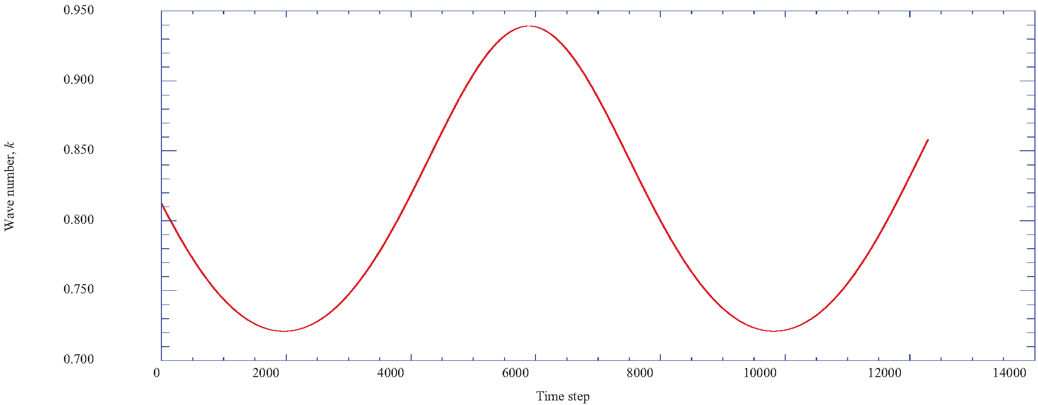
Figure 3 presents the resulting time dependent wave number as a function of time step over the complete computation range. It should be noted that the wave number is a continuously varying parameter throughout the computations of the boundary layer instabilities.

Figure 3. The time dependent wave number, k, is shown as a function of the time step. Parameters: α = 1.00, ω = 8.00.

Figure 3. The time dependent wave number, k, is shown as a function of the time step. Parameters: α = 1.00, ω = 8.00.

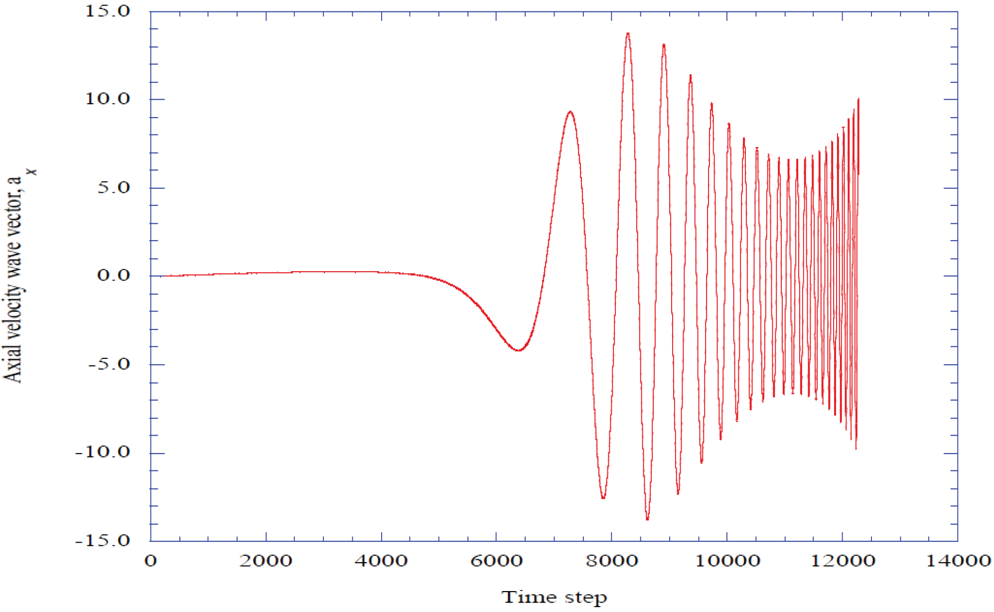
Figure 4 presents the variation of the fluctuating axial velocity wave vector as a function of the time step. These results indicate that after a period of induction, oscillatory instabilities develop in the fluctuating axial velocity wave vector.

Figure 4. The axial velocity wave vector is shown as a function of the time step. Parameters: x = 0.08, z = 0.003, η = 1.402, K = 0.20, α = 1.00, ω = 8.00.

Figure 4. The axial velocity wave vector is shown as a function of the time step. Parameters: x = 0.08, z = 0.003, η = 1.402, K = 0.20, α = 1.00, ω = 8.00.

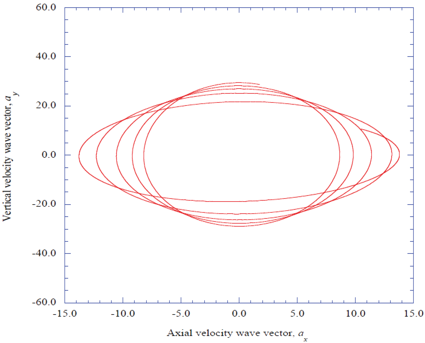
Figure 5 presents the phase diagram of the fluctuating vertical velocity wave vector as a function of the fluctuating axial velocity wave for the complete range of time step values. Two separate regions are indicated. The first region indicates a rather uniform oscillation of the velocity wave vectors, while the second region indicates the presence of ordered structures. The analysis of the spectral entropy rate production will focus on the second of the two regions.

4.2. The Prediction of Spectral Entropy Rates from the Deterministic Results

The results from the time integration of the modified Townsend equations for the various values of the control parameters consist of nonlinear time series outputs for the composite wave number and for the three fluctuating velocity wave vectors. It becomes necessary to process these time series records to extract the underlying structural characteristics of the time series. Chen [11] has presented a series of studies of methods for the extraction of such structural information from time series information. In reference [11], a computer source code was presented which implemented the maximum entropy method (Burg’s method) for spectral analysis of geophysical seismic time data records. This method considerably improves the spectral resolution for short records.

Figure 5. The vertical velocity wave vector is shown as a function of the axial velocity wave vector. Parameters: x = 0.08, z = 0.003, η = 1.402, K = 0.20, α = 1.00, ω = 8.00.

Figure 5. The vertical velocity wave vector is shown as a function of the axial velocity wave vector. Parameters: x = 0.08, z = 0.003, η = 1.402, K = 0.20, α = 1.00, ω = 8.00.

Burg’s method has its theoretical roots in information theory [35], where a discussion and a proof of Burg’s maximum entropy rate theorem are given. These authors also make reference to the work of Rissanen [36,37], where the maximum entropy method is related to the concept of Kolmogorov complexity [38].

One of the significant advantages of Burg’s method is the enhancement of the spectral peaks in the power spectral density distribution. Our previous experience with Burg’s method and the existence of useful source codes for the analysis of the predicted time series led to our use of this method for the evaluation of the power spectral density of the x-y kinetic energy, a_x² + a_y², for each segment in the time series. A series of time segments representing an internal block of data with 2048 data points from time steps 8192 to 10240 is used for the evaluation of the underlying structure embedded in the output nonlinear time series data.

The method of computation used for the prediction of the distribution of the power spectral density rates is the method presented by Press, et al. [39]. The individual histories for the fluctuating axial and vertical velocity wave-vector components are combined into one time series by adding the squares of each component for each time step. The selected time series is then divided into 64 segments with 32 data sets per segment. Burg’s method [38], is then applied to each segment of the 32 data sets to obtain 16 spiked values of the power spectral density of the kinetic energy, $f_r$, for each particular segment.

At this point, it becomes necessary to introduce an appropriate measure by which we can obtain information that characterizes the effect of each of the control parameters in the boundary layer profiles and in the imposed pressure disturbances in producing boundary layer instabilities. This measure is the spectral entropy rate evaluated in each of the time segments for which the power spectral density of the local kinetic energy has been determined.

The probability value of each set of particular spectral densities for each segment is first computed from $P_r=f_r/{\displaystyle \sum _r{f}_r}$.

The methods of Powell and Percival [13], Grassberger and Procaccia [40], and Cohen and Procaccia [41] are then applied to the probability distributions for each time segment to develop the spectral entropy rate for the given segment. The spectral entropy rate (1/s) is then defined for the j-th time segment as:

$$s_j\_spent=-{\displaystyle \sum _r{P}_r}\ln P_r$$

(41)

This procedure is applied to each of the 64 segments over the selected time data range.

For the spectral entropy rate results that will be presented, we should note the results are presented over the 64 time data segments of the 2,048 time steps block of nonlinear time series output at specified locations, either at a normalized vertical station or for a particular span wise z location at the axial station of nx = 4 (x = 0.08). These results will show low values of spectral entropy rate production indicating transient coherent behavior, separated by transient pulses of high spectral entropy rate production, through the selected block of time series data. Thus, for the selected location in spatial coordinates, and for the particular set of control parameters, the instability results will be indicated by a time-dependent transition process between chaotic states, to coherent states, returning to chaotic states for each particular system. As indicated in Figure 5, the magnitudes of the a_x and a_y wave vectors are significant, thus representing a largely vertical burst of fluctuating fluid elements.

Figure 6 plots the phase plane behavior of the vertical velocity wave vector, a_y, versus the axial velocity wave vector, a_x, at the transformed vertical location of j = 8 (η = 1.402), over the selected block of time-series data. These results indicate that the effects of the external periodic disturbance are transmitted through the entire boundary layer structure.

The spectral entropy rate results for the phase diagram in Figure 6 are shown in Figure 7. The coherent structures are indicated by the essentially zero values of the spectral entropy rates, while the chaotic sheaths are represented by the peaked values of the spectral entropy rates.

Figure 8 presents the number of spectral entropy rate pulses that occur within the given block of time step data as a function of the span wise location at which the z-y plane velocity gradients are calculated. The prediction of the boundary-layer instabilities is a sensitive function of the span wise location for the evaluation of the velocity gradients in the z-y plane. The results presented in Figure 8 indicate that the location for the evaluation of these gradients must be very near the central x-y plane where the axial and vertical velocity gradients are evaluated.

Figure 9 presents the number of spectral entropy rate pulses that occur as a function of the linearization factor, K.

Figure 6. The vertical velocity wave vector is shown as a function of the axial velocity wave vector for the selected block of time step data. Parameters: x = 0.08, z = 0.003, η = 1.402, K = 0.20, α = 1.00, ω = 8.00.

Figure 6. The vertical velocity wave vector is shown as a function of the axial velocity wave vector for the selected block of time step data. Parameters: x = 0.08, z = 0.003, η = 1.402, K = 0.20, α = 1.00, ω = 8.00.

Figure 7. The spectral entropy rate is shown as a function of the time segment number. Parameters: x = 0.08, z = 0.003, η = 1.402, K = 0.20, α = 1.00, ω = 8.00.

Figure 7. The spectral entropy rate is shown as a function of the time segment number. Parameters: x = 0.08, z = 0.003, η = 1.402, K = 0.20, α = 1.00, ω = 8.00.

Figure 8. The number of spectral entropy rate pulses is shown as a function of the span wise location for the z-y velocity gradients. Parameters: x = 0.08, η = 1.402, K = 0.20, α = 1.00, ω = 8.00.

Figure 8. The number of spectral entropy rate pulses is shown as a function of the span wise location for the z-y velocity gradients. Parameters: x = 0.08, η = 1.402, K = 0.20, α = 1.00, ω = 8.00.

Figure 9. The number of spectral entropy rate pulses is shown as a function of the linearization factor. Parameters: x = 0.08, z = 0.003, η = 1.402, α = 1.00, ω = 8.00.

Figure 9. The number of spectral entropy rate pulses is shown as a function of the linearization factor. Parameters: x = 0.08, z = 0.003, η = 1.402, α = 1.00, ω = 8.00.

For K = 1.0, the factor F is set equal to unity to enforce the elimination of the nonlinear coupling terms from the deterministic equations. The results presented in Figure 9 indicate that non-linear coupling terms must be included in the coupled, deterministic equations for the fluctuating velocity wave vectors for the solutions to present any information about resulting boundary-layer instabilities. If the coupled, deterministic equations do not include any non-linear effects (if F = 1.0), the solutions will provide no information about boundary-layer instabilities.

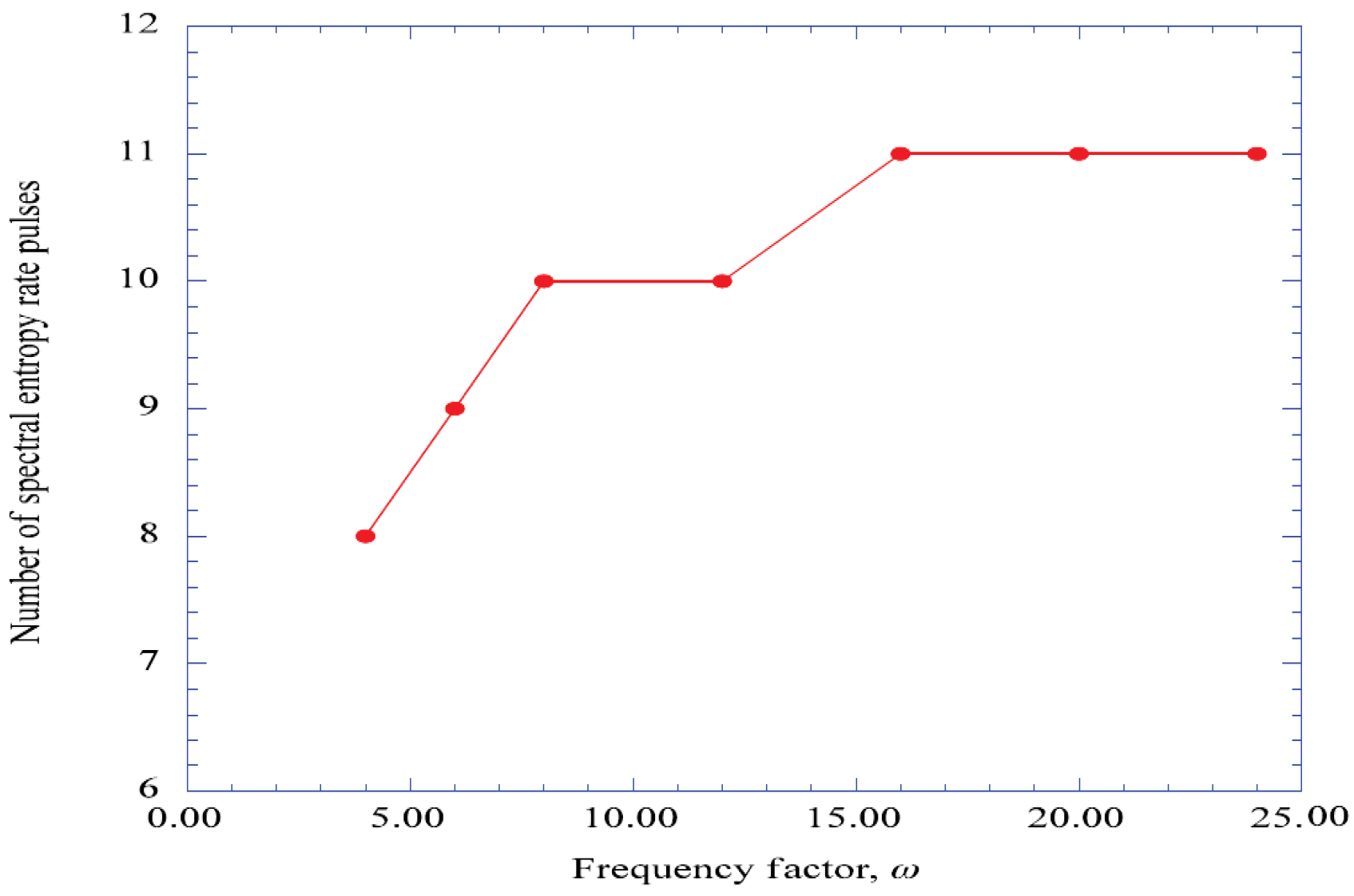
Figure 10 presents the number of spectral entropy rate pulses as a function of the applied frequency factor, ω. These results indicate that as the frequency factor is increased, the rate of production of ordered structures separated by regions of chaotic behavior increases.

Figure 10. The number of spectral entropy rate pulses is shown as a function of the frequency factor. Parameters: x = 0.08, z = 0.003, η = 1.402, K = 0.20, α = 1.00.

Figure 10. The number of spectral entropy rate pulses is shown as a function of the frequency factor. Parameters: x = 0.08, z = 0.003, η = 1.402, K = 0.20, α = 1.00.

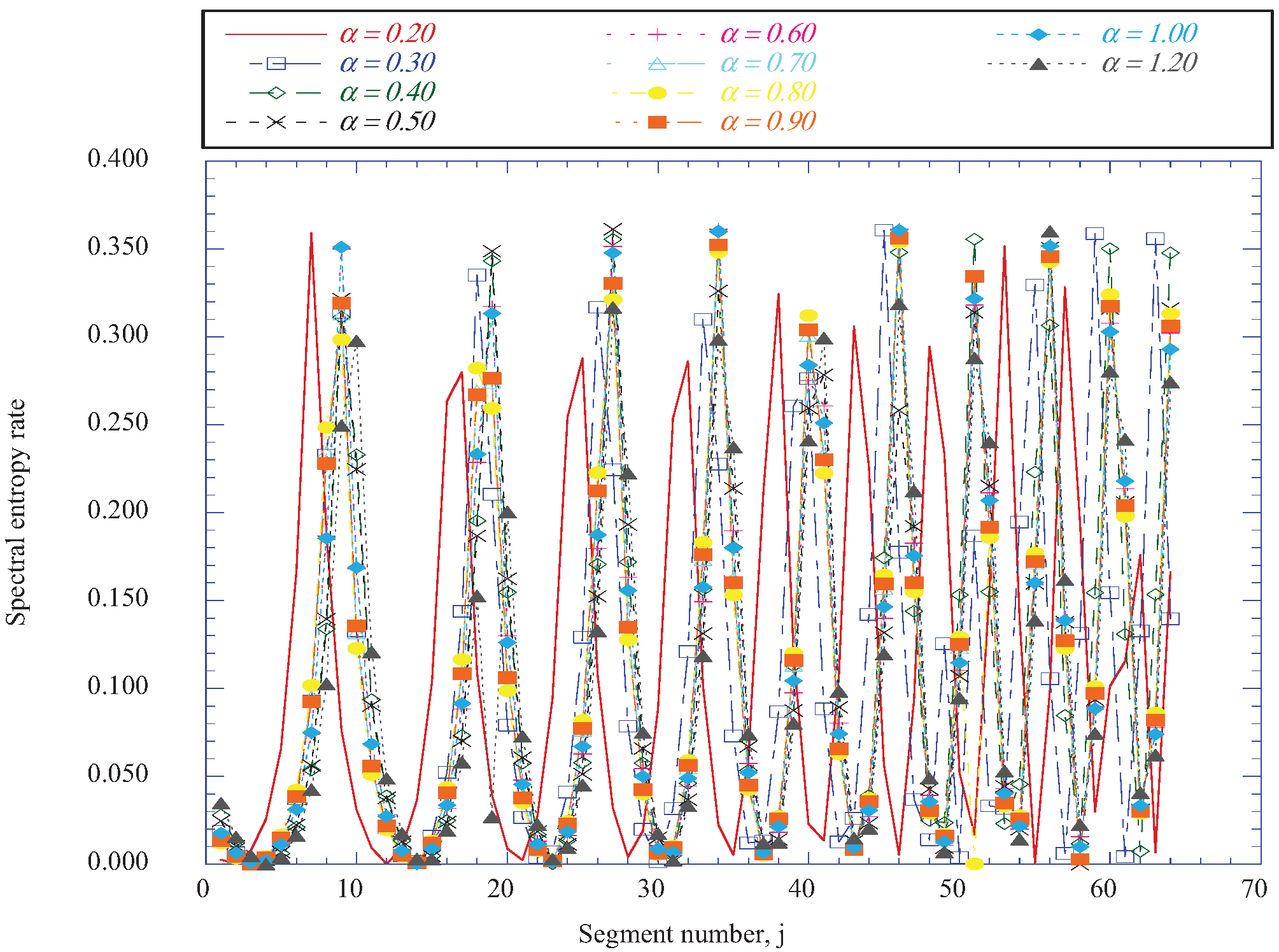
Figure 11 presents an overlay of the spectral entropy rates for various values of the applied amplification factor, α, across the given block of time step data. Apparently, the generation of transient coherent structures within the boundary layer is not a strong function of the amplitude of the imposed pressure disturbance, but more a function of the frequency of the applied disturbance.

For a given set of control parameters, an interesting question concerns the transient generation of coherent structures at various vertical locations across the boundary layer. The spectral entropy rates at several values of normalized vertical dimension, η, have been determined and are presented in Figure 12, Figure 13 and Figure 14. Near the wall, at η = 0.200, the rapid production of coherent and chaotic structures is indicated in Figure 12. As we move further out in the boundary layer, at η = 1.402, the coherent structures are more prominent, with a smaller number of pulses of chaotic behavior in between, as indicated in Figure 7. However, at the vertical location of η = 2.206, the rapid production of smaller transient coherent structures occurs again, as indicated in Figure 13. Finally, at the vertical location of η = 3.414, Figure 14 indicates transient coherent structures of significant duration, with only several pulses of high spectral entropy rate production separating the coherent regions. Beyond the boundary layer location of η = 4.221, the solutions of the nonlinear deterministic equations do not indicate the presence of instabilities [5].

Figure 11. The spectral entropy rate values are shown for several values of the applied amplification factor for the imposed pressure disturbance. Parameters: x = 0.08, z = 0.003, η = 1.402, K = 0.20, ω = 8.00.

Figure 11. The spectral entropy rate values are shown for several values of the applied amplification factor for the imposed pressure disturbance. Parameters: x = 0.08, z = 0.003, η = 1.402, K = 0.20, ω = 8.00.

Figure 12. The spectral entropy rate is shown for the vertical location of η = 0.200. Parameters: x = 0.08, z = 0.003, η = 0.200, K = 0.20, α = 1.00, ω = 8.00.

Figure 12. The spectral entropy rate is shown for the vertical location of η = 0.200. Parameters: x = 0.08, z = 0.003, η = 0.200, K = 0.20, α = 1.00, ω = 8.00.

Figure 13. The spectral entropy rate is shown for the vertical location of η = 2.206. Parameters: x = 0.08, z = 0.003, η = 2.206, K = 0.20, α = 1.00, ω = 8.00.

Figure 13. The spectral entropy rate is shown for the vertical location of η = 2.206. Parameters: x = 0.08, z = 0.003, η = 2.206, K = 0.20, α = 1.00, ω = 8.00.

Figure 14. The spectral entropy rate is shown for the vertical location of η = 3.414. Parameters: x = 0.08, z = 0.003, η = 3.414, K = 0.20, α = 1.00, ω = 8.00.

Figure 14. The spectral entropy rate is shown for the vertical location of η = 3.414. Parameters: x = 0.08, z = 0.003, η = 3.414, K = 0.20, α = 1.00, ω = 8.00.

The integration in time of the modified Townsend equations yields the time series of the fluctuating axial, vertical and span wise velocity wave vectors. These series are oscillatory in nature. The maximum magnitude of the vertical velocity wave vector decreases from a significant level near the wall to a much lower level further out in the boundary layer. Figure 15 presents values of the maximum vertical velocity wave vector for several vertical boundary layer stations as a function of the applied frequency factor.

Figure 15. The maximum amplitude of the vertical velocity wave vector is shown for several vertical locations in the boundary layer as a function of the frequency factor. Parameters: x = 0.08, z = 0.003, K = 0.20, α = 1.00.

Figure 15. The maximum amplitude of the vertical velocity wave vector is shown for several vertical locations in the boundary layer as a function of the frequency factor. Parameters: x = 0.08, z = 0.003, K = 0.20, α = 1.00.

6. Discussion

Considerable progress has been made in the development of hypersonic propulsion systems. In the development process, it has been found that unsteady shock interactions can occur on blunt body forms of parts of the inlet structure. These interactions produce pressure disturbances that are imposed on the underlying subsonic boundary layer, which is formed over the body surface. The fluctuating vertical velocity wave vectors shown in Figure 15 are orders of magnitude greater near the wall as compared with the values near the region of transient coherent structure production. These results indicate that the boundary layer velocity gradients near the wall are much more receptive to the imposed pressure disturbances than are the outer regions of the boundary layer.

By embedding modified Townsend equations for the fluctuating velocity wave vectors in the laminar boundary layer environments in both the axial and the span wise planes, and introducing sets of internal and external control parameters, it has been shown that these boundary layers are receptive to the imposed pressure disturbances.

The spectral entropy rates, determined from the resulting nonlinear time series describing the fluctuating velocity wave vectors, indicate the production of transient chaotic, coherent, and then chaotic flow structures at each normalized vertical boundary layer location examined.

In a study of the core dynamics of coherent vortex structures, Pradeep and Hussain [42] describe the formation of thin sheaths of intense vorticity surrounding regions of low enstrophy, which we have described as coherent structures. These sheaths collapse and form with the onset and dispersal of the regions of coherent structures. The sharp peaks of the spectral entropy rates apparently represent sharp boundaries between the formation and the dissolution of the regions of coherent structures. Since the peaks represent a sharp break from one structure to the next, they must represent distinct boundaries in the nature of the flow structures. Thus, for a specific location in the boundary layer, and for a given set of control parameters, the time-dependent values of the various wave number vectors and the variation of the total wave number induce a time sequence of the generation of flow structures, each consisting of a sheath of chaotic motion undergoing a transition to a coherent structure, which then undergoes transition to a following sheath of chaotic flow structure. The sharp peaks in the spectral entropy pulses apparently indicate that each flow structure is individually separate from the others.

It is particularly interesting to note that for each of vertical boundary layer location and each set of control parameters examined, the spectral entropy rate pulses have a maximum value in the range of 0.325 ± 0.02. An asymptotic value of 0.325 ± 0.02 for the Kolmogorov entropy for the Hénon map is given in [41]. The positive nature of the spectral entropy rates in our results thus implies chaotic behavior within the pulses. Thus, the results obtained for the boundary layer instabilities indicate the production of transient coherent structures separated by regions of chaotic transitions. For the vertical station j = 22 (η = 4.221), no instabilities are observed (Figure 15 of [5]). We have not explored the outer part of the boundary layer.

7. Conclusions

The complete set of equations for the fluctuating velocity wave vectors within a boundary-layer flow has been reduced to a set of equations similar to the Lorenz equations with the introduction of sets of internal and external control parameters. The internal control parameters are the velocity gradients for the vertical boundary-layer stations in both the x-y and z-y planes, the z location for the z-y velocity gradients and the linearization factor K in the modified Townsend equations. The external parameters are the frequency factor and the amplification factor of the imposed pressure disturbance from the blunt body unsteady shock interaction process. The measure for the effect of the values of the various control parameters is the spectral entropy rate calculated from the power spectral density properties of the nonlinear time series output of the deterministic equations. For a given set of internal and external control parameters, the spectral entropy rate results show time-dependent transitions from chaotic to coherent motion, then back to chaotic motion, in a repetitive manner within the nonlinear time-series output. The results indicate that the Falkner-Skan boundary layer profiles in both the x-y and the z-y plane are required for the prediction of the boundary-layer instabilities. For the z-position control parameter, the transition rates are high for the z location nearest the x-y plane, decreasing as the location moves away from the x-y plane. For the linearization parameter near zero (with the full nonlinear terms included in the deterministic equations), the transition rates are high, while vanishing completely when the nonlinear terms are eliminated from the equations. For the external control parameters, the frequency factor has the dominant effect, increasing the rate of spectral entropy production as the frequency factor increases in value. The external amplification factor seems to have essentially little effect on the spectral entropy rate production. Three important observations can be noted from these results: First, the spectral entropy rate pulses have positive values in the range of 0.325 ± 0.020, indicating possible transient chaotic sheath behavior surrounding the coherent core of the structures. Second, spectral entropy rates at vertical locations just below the midpoint on the η scale indicate the time-dependent production of significant vortex-like structures, and third, the maximum vertical velocity wave vector magnitudes appear significantly higher near the surface than in the vortex-like production regions. This result has particular significance for surface heat-transfer considerations.

References

- Klimontovich, Y.L.; Bonitz, M. Definition of the degree of order in selforganization processes. Annalen der Physik 1988, 7, 340–352. [Google Scholar] [CrossRef]
- Kapitaniak, T. Controlling Chaos; Academic Press Inc.: San Diego, CA, USA, 1996. [Google Scholar]
- Pyragas, K. Continuous control of chaos by self-controlling feedback. Phys. Lett. A 1990, 170, 421–427. [Google Scholar] [CrossRef]
- Pyragas, K. Predictable chaos in slightly perturbed unpredictable chaotic systems. Phys. Lett. A 1993, 181, 203–210. [Google Scholar] [CrossRef]
- Isaacson, L.K. Spectral entropy in a boundary-layer flow. Entropy 2011, 13, 402–421. [Google Scholar] [CrossRef]
- Panaras, A.G.; Drikakis, D. High-speed unsteady flows around spiked-blunt bodies. J. Fluid Mech. 2009, 63, 69–96. [Google Scholar] [CrossRef]
- Drikakis, D.; Rider, W. High-Resolution Methods for Incompressible and Low-Speed Flows; Springer-Verlag: Berlin, Germany, 2005. [Google Scholar]
- Lind, C.A.; Lewis, M.J. Computational analysis of the unsteady type IV shock interaction of blunt body flows. J. Propul. Power 1996, 12, 127–133. [Google Scholar] [CrossRef]
- Lind, C.A. Effect of geometry on the unsteady type IV shock interaction. J. Aircraft 1997, 34, 64–71. [Google Scholar] [CrossRef]
- Townsend, A.A. The Structure of Turbulent Shear Flow, 2nd ed.; Cambridge University Press: Cambridge, UK, 1976; pp. 45–49. [Google Scholar]
- Chen, C.H. Digital Waveform Processing and Recognition; CRC Press, Inc.: Boca Raton, FL, USA, 1982; pp. 131–158. [Google Scholar]
- Press, W.; Teukolsky, S.A.; Vetterling, W.T.; Flannery, B.P. Numerical Recipes in C: The Art of Scientific Computing, 2nd ed.; Cambridge University Press: Cambridge, UK, 1992; pp. 572–575. [Google Scholar]
- Powell, G.E.; Percival, I.C. A spectral entropy method for distinguishing regular and irregular motions for Hamiltonian systems. J. Phys. Math. Gen. 1979, 12, 2053–2071. [Google Scholar] [CrossRef]
- Anderson, J.D., Jr. Hypersonic and High-Temperature Gas Dynamics, 2nd ed.; American Institute of Aeronautics and Astronautics, Inc.: Reston, VA, USA, 2006; pp. 395–406. [Google Scholar]
- Ben-Dor, G. Shock Wave Reflection Phenomena, 2nd ed.; Springer-Verlag: Berlin, Germany, 2007. [Google Scholar]
- Zucrow, M.J.; Hoffman, J.D. Gas Dynamics; John Wiley & Sons, Inc.: New York, NY, USA, 1976; Volume 1, pp. 708–709. [Google Scholar]
- Zucrow, M.J.; Hoffman, J.D. Gas Dynamics; John Wiley & Sons, Inc.: New York, NY, USA, 1976; Volume 1, pp. 335–349. [Google Scholar]
- Truitt, R.W. Fundamentals of Aerodynamic Heating; Ronald Press Company: New York, NY, USA, 1960; pp. 9–20. [Google Scholar]
- Heywood, J.B. Internal Combustion Engine Fundamentals; McGraw-Hill Book Company: New York, NY, USA, 1988; pp. 130–135. [Google Scholar]
- Zucrow, M.J.; Hoffman, J.D. Gas Dynamics; John Wiley & Sons, Inc.: New York, NY, USA, 1976; Volume 1, pp. 20–23. [Google Scholar]
- Mills, A.F. Heat Transfer; Richard D. Irwin, Inc.: Boston, MA, USA, 1992; pp. 824–827. [Google Scholar]
- Dorrance, W.H. Viscous Hypersonic Flow; McGraw-Hill Book Company, Inc.: New York, NY, USA, 1962; pp. 276–315. [Google Scholar]
- Cebeci, T.; Bradshaw, P. Momentum Transfer in Boundary Layers; Hemisphere: Washington, DC, USA, 1977. [Google Scholar]
- Hansen, A.G. Similarity Analyses of Boundary Value Problems in Engineering; Prentice-Hall, Inc.: Englewood Cliffs, NJ, USA, 1964; pp. 86–92. [Google Scholar]
- Durbin, P; Zaki, T. Continuous mode transition. In Transition and Turbulence Control; Gad-el-Hak, M., Tsai, H.M., Eds.; World Scientific Pub. Co.: Singapore, 2006; pp. 87–106. [Google Scholar]
- Andersson, P.; Berggren, M.; Henningson, D.S. Optimal disturbances and bypass transition in boundary layers. Phys. Fluids 1999, 11, 134–150. [Google Scholar] [CrossRef]
- Corbett, P.; Bottaro, A. Optimal perturbations for boundary layers subject to stream-wise pressure gradient. Phys. Fluids 2000, 12, 120–130. [Google Scholar] [CrossRef]
- Brandt, L.; de Lange, H.C. Streak interactions and breakdown in boundary layer flows. Phys. Fluids 2008, 20, 024107. [Google Scholar] [CrossRef]
- Hoepffner, J.; Brandt, L. Stochastic approach to the receptivity problem applied to bypass transition in boundary layers. Phys. Fluids 2008, 20, 024108. [Google Scholar] [CrossRef]
- Schlatter, P.; Brandt, L.; de Lange, H.C.; Henningson, D.S. On streak breakdown in bypass transition. Phys. Fluids 2008, 20, 101505. [Google Scholar] [CrossRef]
- Landau, L.D.; Lifshitz, E.M. Quantum Mechanics: Non-Relativistic Theory; Pergamon Press, Ltd.: London, UK, 1958; pp. 133–144. [Google Scholar]
- Hellberg, C.S.; Orszag, S.A. Chaotic behavior of interacting elliptical instability modes. Phys. Fluids 1988, 31, 6–8. [Google Scholar] [CrossRef]
- Isaacson, L.K. Deterministic prediction of the entropy increase in a sudden expansion. Entropy 2011, 13, 402–421. [Google Scholar] [CrossRef]
- Press, W.; Teukolsky, S.A.; Vetterling, W.T.; Flannery, B.P. Numerical Recipes in C: The Art of Scientific Computing, 2nd ed.; Cambridge University Press: Cambridge, UK, 1992; pp. 710–714. [Google Scholar]
- Cover, T.M.; Thomas, J.A. Elements of Information Theory, 2nd ed.; John Wiley & Sons, Inc.: Hoboken, NJ, USA, 2006; pp. 415–421. [Google Scholar]
- Rissanen, J. Complexity and information in data. In Entropy; Greven, A., Keller, G., Warnecke, G., Eds.; Princeton University Press: Princeton, NJ, USA, 2003; pp. 299–327. [Google Scholar]
- Rissanen, J. Information and Complexity in Statistical Modeling; Springer Science+Business Media, LLC: New York, NY, USA, 2007. [Google Scholar]
- Li, M.; Vitányi, P. An Introduction to Kolmogorov Complexity and Its Applications; Springer Science+Business Media, LLC: New York, NY, USA, 2008. [Google Scholar]
- Grassberger, P.; Procaccia, I. Estimation of the Kolmogorov entropy from a chaotic signal. Phys. Rev. A 1983, 28, 2591–2593. [Google Scholar] [CrossRef]
- Cohen, A.; Procaccia, I. Computing the Kolmogorov entropy from time signals of dissipative and conservative dynamical systems. Phys. Rev. A 1985, 31, 1872–1882. [Google Scholar] [CrossRef] [PubMed]
- Pradeep, D.S.; Hussain, F. Core dynamics of a coherent structure: A protypical physical-space cascade mechanism? In Turbulence Structure and Vortex Dynamics; Hunt, J.C.R., Vassilicos, J.C.R., Eds.; Cambridge University Press: New York, NY, USA, 2011; pp. 54–82. [Google Scholar]
© 2012 by the authors; licensee MDPI, Basel, Switzerland. This article is an open access article distributed under the terms and conditions of the Creative Commons Attribution license (http://creativecommons.org/licenses/by/3.0/).
Share and Cite
MDPI and ACS Style
Isaacson, L.K. Control Parameters for Boundary-Layer Instabilities in Unsteady Shock Interactions. Entropy 2012, 14, 131-160. https://doi.org/10.3390/e14020131
AMA Style
Isaacson LK. Control Parameters for Boundary-Layer Instabilities in Unsteady Shock Interactions. Entropy. 2012; 14(2):131-160. https://doi.org/10.3390/e14020131
Chicago/Turabian StyleIsaacson, LaVar King. 2012. "Control Parameters for Boundary-Layer Instabilities in Unsteady Shock Interactions" Entropy 14, no. 2: 131-160. https://doi.org/10.3390/e14020131