Disentangling Complexity from Randomness and Chaos

Department of History and Philosophy of Science, University of Cambridge, Free School Lane, CB2 3RH Cambridge, UK
Entropy 2012, 14(2), 177-212; https://doi.org/10.3390/e14020177
Submission received: 27 December 2011
/
Revised: 26 January 2012
/
Accepted: 31 January 2012
/
Published: 7 February 2012
(This article belongs to the Special Issue Arrow of Time)
Abstract
:This study aims to disentangle complexity from randomness and chaos, and to present a definition of complexity that emphasizes its epistemically distinct qualities. I will review existing attempts at defining complexity and argue that these suffer from two major faults: a tendency to neglect the underlying dynamics and to focus exclusively on the phenomenology of complex systems; and linguistic imprecisions in describing these phenomenologies. I will argue that the tendency to discuss phenomenology removed from the underlying dynamics is the main root of the difficulties in distinguishing complex from chaotic or random systems. In my own definition, I will explicitly try to avoid these pitfalls. The theoretical contemplations in this paper will be tested on a sample of five models: the random Kac ring, the chaotic CA30, the regular CA90, the complex CA110 and the complex Bak-Sneppen model. Although these modelling studies are restricted in scope and can only be seen as preliminary, they still constitute on of the first attempts to investigate complex systems comparatively.
1. Introduction
“Was sich überhaupt sagen läßt, läßt sich klar sagen; und wovon man nicht reden kann, darüber muß man schweigen.”(L. Wittgenstein, Tractatus Logico-Philosophicus)
During the last ten years complexity research has received a relatively large amount of attention by both the scientific community and the general public: Paramount scientific figures like Nobel Laureate Murray Gell-Mann have championed its cause (e.g., [1]); Science magazine devoted a special issue to it; and in the 2004’s bestseller lists, The Swarm [2] explored the sinister consequences of not paying enough attention to complex systems.
One of the greatest draws of complexity as a field of research is the possibility of recognizing it in virtually every branch of science and the social sciences (e.g., [3]). However, despite the labelling of an increasingly large number of models and natural systems as “complex”, the definition of the term has remained vague. Standish [4] pointed out that these difficulties extend to both a qualitative identification of a conclusive set of defining features that a complex system should possess, as well as to the quantitative measurements of complexity as a property. The difficulty of finding an unequivocal conceptualization and measure of complexity is also recognized by Gell-Mann [5], who states that (p. 1):
“[A] variety of different measures would be required to capture all our intuitive ideas about what is meant by complexity and by its opposite, simplicity.”
In fact, Lloyd [6] enumerates forty-two different existing complexity measures in what is described as “a nonexhaustive list” (p. 7).
Despite the lack of agreement on the definition of complexity, complexity scientists have been eager to stress the importance of the concept as central to nature. For example, Wolfram [7] writes about his work:
“Perhaps the most dramatic [benefit] is that it yields a resolution to what has long been considered the single greatest mystery of the natural world: what secret is it that allows nature seemingly so effortlessly to produce so much that appears to us complex.”(p. 2)
However, the failure to precisely state what it actually is that needs to be studied in order to unravel “nature’s greatest mystery” has drawn extensive criticism. Horgan [8] describes complexity as an unjustifiably hyped “pop-science movement” that spun off from chaos theory. A closer review of the complexity measures compiled by Lloyd [6] reveals that they indeed borrow heavily from a number of “ancestor theories” like statistical mechanics, chaos theory and computational physics. Likewise, a closer look at the conception of these measures reveals that the struggle for a definition of complexity is fueled by two factors: a failure to fully emancipate oneself from these epistemological ancestors and the uncritical use of metaphorical and imprecise language.
This paper aims to present a structured account of the “intuitive ideas of what is meant by complexity” mentioned by Gell-Mann [5]. With the possible exception of the currently mostly speculative work by Wolfram [7], intuitions about complexity have been largely restricted to its phenomenology. I will argue that the tendency to discuss phenomenology removed from the underlying dynamics is the main root of the difficulties in distinguishing chaotic from complex systems. I will claim that a purely dynamical definition of complexity is possible, however, it would be more inclusive than the complexity community wishes it to be. Instead, a phenomenological sieve must be imposed to distinguish the “interesting” systems from “simple” ones with similar dynamics.
Secondly, I will show that both previous attempts to design such a sieve as well as the general complexity discourse suffer from either semantic circularities or an over-reliance on metaphorical language, which seems to compensate for a potentially fundamental difficulty in arriving at an objective description. It will also be shown that quantitative complexity measures based on the most prevalent metaphors are not successful in identifying complex models as such. As indicated by the mildly ironic motto of this paper I believe that it would have aided the the progress of complexity science if the community had refrained from hiding the inability to recognize the essence of complexity behind eye-catching but fundamentally imprecise phrases.
Based on the insights gained in the first parts of this paper, we will finally design our own complexity definition.
Methodologically, I complement my theoretical investigation by the analysis of a sample of five simple models. The phenomenologies of two of these are generally judged to be complex: the Wolfram Cellular Automaton (CA) 110 (e.g., [7]) and a discrete Bak-Sneppen model [9]. I have deliberately sought to include models that are based on very different dynamical premises (e.g., the CA110 is deterministic while the Bak-Sneppen model is probabilistic), thereby hoping to address a lacuna in comparative complexity studies. In addition to these I will consider: the Wolfram CA30, a model with pseudo-random (often called “chaotic”) output; the Kac ring, a dynamically random and phenomenologically entropy-maximizing model; and the Wolfram CA90, a model with regular phenomenology. The models will be used as both a means of verifying existing assumptions about complexity as well as a testbed for my own ideas. Underlying the reliance on these simple computer models is the assumption that complexity science can still very much be identified with the study of such simulations (e.g., [10]).
In Section 2 I will describe the models used in this study. Section 3 contains a discussion of dynamical complexity definitions and measures. In Section 4 I will examine qualitative and quantitative descriptions of complex phenomenology. Conclusions will be drawn in Section 5, which also contains my attempt at a rudimentary complexity definition.
2. Five Simple Models
In this section I will describe the five simple models used in this study. Wherever possible, the models have been chosen as typical, or even well-known, representatives of a larger class of such simulations. I have also deliberately included both a deterministic as well as probabilistic complex model.
2.1. The Kac Ring
The Kac model was developed by Kac [11] as a means of demonstrating that coarse graining and Stosszahlansatz-like dynamical assumptions can lead to irreversible evolution of a macroscopic entropy. It describes an idealized system of particles whose phase-space values are determined by randomized collisions only. Dorfmann [12] and Gottwald and Oliver [13] provide a detailed discussion of the dynamics of the system in the context of thermodynamics and statistical physics. My abbreviated account below is based on their exposition.
The KAC model consists of a one-dimensional, periodic lattice of N sites arranged around a ring. Each site is occupied by a particle, which has either the property “black” or the property “white”. Neighbouring sites are joined by edges. Each of the N edges is assigned one of two markers, which will be denoted as S and .
The dynamics of the system is discrete and consists of particles moving clockwise to the neighbouring site. Thereby, the edge markers control the evolution of the colour property: a particle changes colour if it traverses an edge marked but remains unchanged if the edge marker is S. If the same number of steps is retraced in the counter-clockwise direction, the initial state is reached again. The dynamics of the ring is therefore reversible. Furthermore, the time evolution of the system is periodic. Depending on the number n of colour-changing edges , states reoccur with a period of N or time-steps for even or odd n, respectively.
Mimicking the dual mode of description employed in statistical physics and thermodynamics, microscopic and macroscopic variables will be used to describe the Kac model. On the macroscopic level, the number B of black particles and the number W of white particles will be used as fundamental variables. On a mesoscale level, convenient properties to consider are the number of black or white particles before an edge: b and w, respectively. From the previous paragraph, the importance of these quantities for the evolution of the model in the next step is immediately apparent: b is equal to the number of particles changing from black to white and w is equal to the number of particles changing from white to black. Since the computation of b and w requires knowledge of the exact location of the particles on the ring, while that of B and W only relies on the overall ratio of particles regardless of their location, the choice of these two pairs of properties is in keeping with the analogy to a microscopic/macroscopic description in statistical mechanics. Using these definitions, the dynamics of the macroscopic quantities are given by the following equations:
and
where t is the discrete time step and constitutes a single, clockwise shift of the ring. Equations (1) and (2) can be combined into a single difference equation:
Since Equation (3) still depends crucially on the microscopic properties b and w, no closed macroscopic description has been achieved.
In order to eradicate these variables one needs to make further assumptions about their relation to the large-scale properties of the system. In analogy to Boltzmann’s Stosszahlansatz, one assumes that each particle is equally likely to experience a “collision” and change its colour property. Noting that the proportion of edges around the ring carrying the marker is given by , one thus assumes that this ratio must also be the probability for a particle to change colour, i.e., one requires:
Since μ can be derived from the macroscopic quantities n and N, we can use Equation (4) to remove the microscopic quantities from Equation (3):
Equation (5) defines a geometric sequence, which can be rewritten as a function of the initial state .
It is notable that Equation (6) is not time reversible, since we necessarily have μ ≤ 1 and therefore 0 for t → ∞. The only exception to this asymptotic behaviour is an initial set-up where the number of S edges equals the number of edges and thus n = , in which case Equation (6) is trivially zero. The Kac model thus captures the time development contrast between macroscopic and microscopic variables that is characteristic of statistical mechanical systems.
2.2. Wolfram Cellular Automata
Von Neumann [14] is generally credited with the invention of cellular automata. However, only after computational resources became more readily available in the 1970s were large-scale studies of such discrete systems conducted. The three cellular automata investigated in this paper belong to a group of one-dimensional, nearest-neighbour automata most extensively studied by Wolfram [7,15,16,17,18,19]. These are particularly suitable for a comparison to the Kac ring since, under periodic boundary conditions, they likewise can be visualised as a ring of black and white particles.
Like the Kac model, Wolfram cellular automata consist of one-dimensional, periodic lattices of N sites arranged around a ring. Each site is again occupied by a particle of either colour “black” or “white”. However, in contrast to the Kac ring, the colour assumed by a particle at position in the next time step t + 1 does not depend on an external property but is determined by the colours of both the given particle as well as its two nearest neighbours at and .
Working with only two colours, there are 2 = 8 different configurations for the colouring of a triplet (, , ). To each of these possibilities a resulting colouring of as either black or white is assigned. The complete set of eight such assignments constitutes the rule set of the given cellular automaton. For the nearest-neighbours set-up with two possible states discussed here, there are 2 = 256 possible rule sets. All of these have been catalogued and named by Wolfram [7]. The naming convention is such that the binary code spelled out by the assigned states (with 1 denoting black and 0 denoting white) of the eight rules is translated into a base 10 number.
In this paper I will consider three of the 256 possible Wolfram cellular automata, CA30, CA90 and CA110. The rule sets for these are given in Table 1.

Table 1.
Wolfram cellular automata rule sets. The upper line shows the parent triplet (, , ), the resulting colouring for is given below. 1 denotes black and 0 denotes white.
| Parent triplet | 1 1 1 | 1 1 0 | 1 0 1 | 1 0 0 | 0 1 1 | 0 1 0 | 0 0 1 | 0 0 0 |
|---|---|---|---|---|---|---|---|---|
| CA 30 | 0 | 0 | 0 | 1 | 1 | 1 | 1 | 0 |
| CA 90 | 0 | 1 | 0 | 1 | 1 | 0 | 1 | 0 |
| CA 110 | 0 | 1 | 1 | 0 | 1 | 1 | 1 | 0 |
2.3. The Bak-Sneppen Model
The Bak-Sneppen model was developed by Bak and Sneppen [20]. It has since become a much-cited example of a system with self-organized criticality (e.g., [21,22,23]) and thus holds at least some epistemological credentials towards a claim of complexity. The natural process the model represents is the co-evolution of a number of species.
In its one-dimensional form, which I will consider for better comparison to the other models discussed, the Bak-Sneppen model consists of a ring of N sites connected to each other by edges. The general set-up is therefore very similar to the Kac model and the Wolfram cellular automata. Each site represents a species with fitness value ( ϵ [0,1]). As in the Wolfram models, the development of connected sites—the triple (, , )—is interlinked, in a crude attempt to capture the evolution of co-dependent species. During a time-step, the site with the lowest fitness value is determined. Its fitness value and those of its two neighbours, and , are then replaced by equi-distributed random numbers on the unit interval. This represents the extinction of the three co-evolving species and their replacement by three new ones. Therefore, in contrast to the Wolfram cellular automata or the Kac ring, not all sites are updated during a time step.
While the classic version of the Bak-Sneppen model uses a continuous spectrum of fitness values, I will consider a discrete version which only employs values of 1 and 0 [9]. This model will be directly comparable to those discussed in the previous sections. In the discrete Bak-Sneppen model, the site to be updated, , is chosen randomly. If = 0 then the triple around is updated by a renewed fitness calculation. Otherwise the ring remains unchanged. This computation randomly assigns either a new fitness value of 1 or 0 to each of the three sites.
2.4. Model Results
I have simulated rings of 100 sites, usually for 200 time steps. A uniformly random distribution of edge markers around the ring (giving μ = 0.51) was used for the Kac ring. The initial state was a single black particle at position . All models were written in FORTRAN. MathCad and the standard Microsoft Office package were used for post-processing.
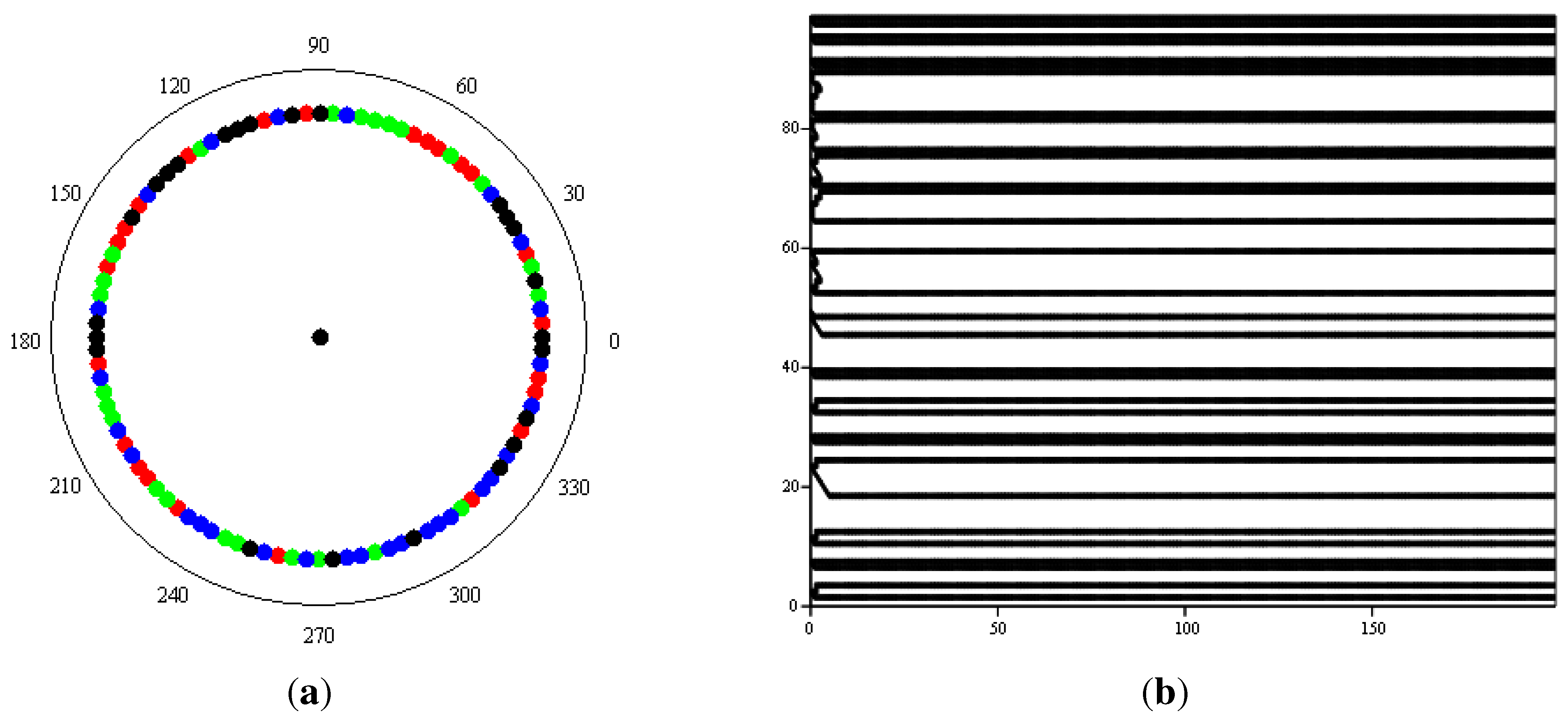
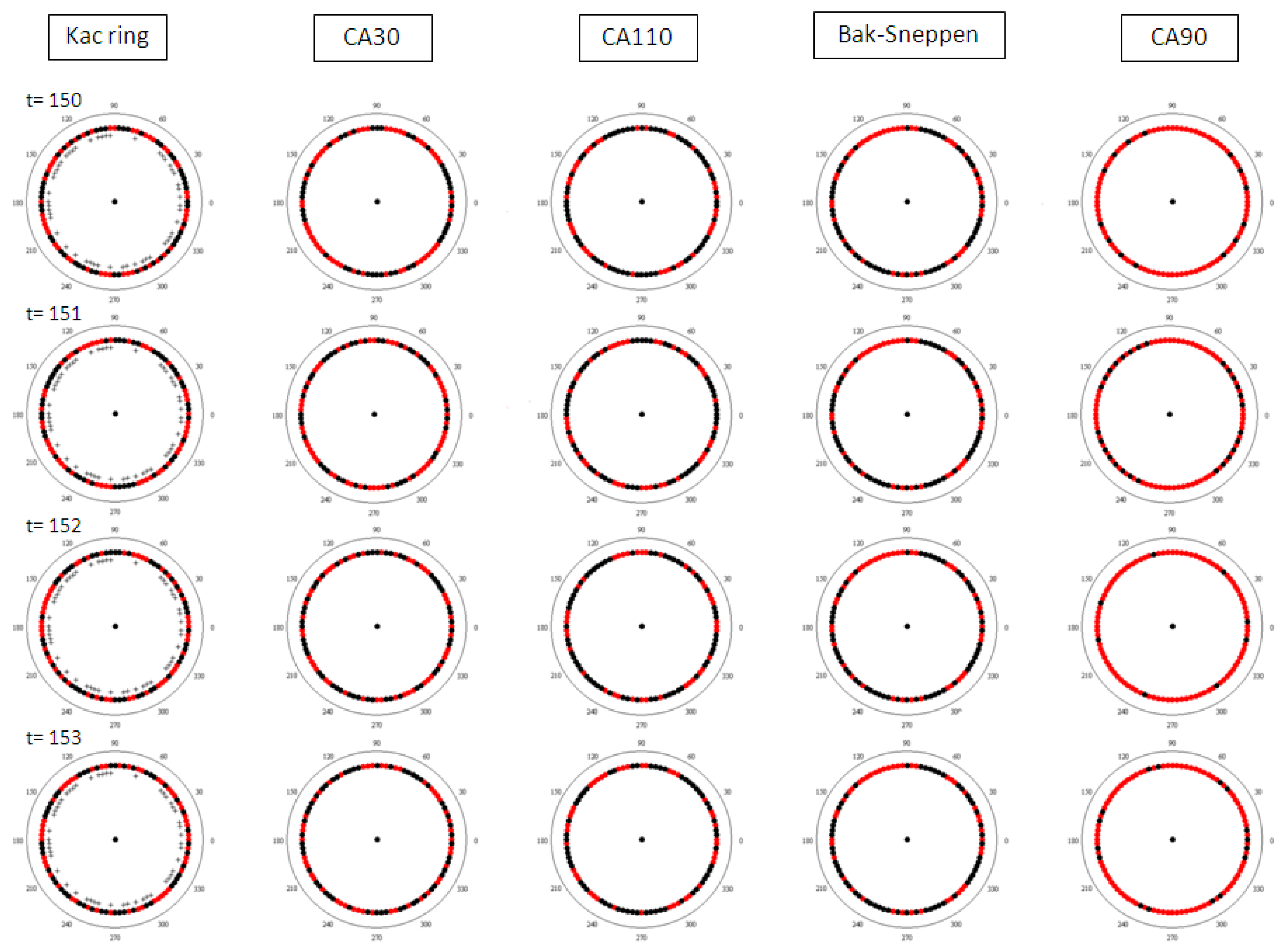
Results from the simulations are summarized in Figure 1 and Figure 2. Figure 1 shows the space-time diagrams for all five models in comparison. In Figure 2 the rings are displayed at the four consecutive time steps between t = 150 and t = 153. A better impression of the phenomenology in this naturalistic representation can be gained by watching the animations appended to this article (Appendix A), which show the full run for each of the five models.
My results for the Kac ring model compare well with those obtained by Gottwald and Oliver [13]. Since the ring features an odd number of markers, it is symmetric with a period of , i.e., the time development repeats itself after 200 time steps. Similarly, my discrete Bak-Sneppen model compares well to previous results with a similar model [9]. The space time diagrams simulated for the Wolfram cellular automata are identical to the ones collected in the literature for the given rules and initialisation (e.g., [7]).
Figure 1.
Space time diagrams of the five models.
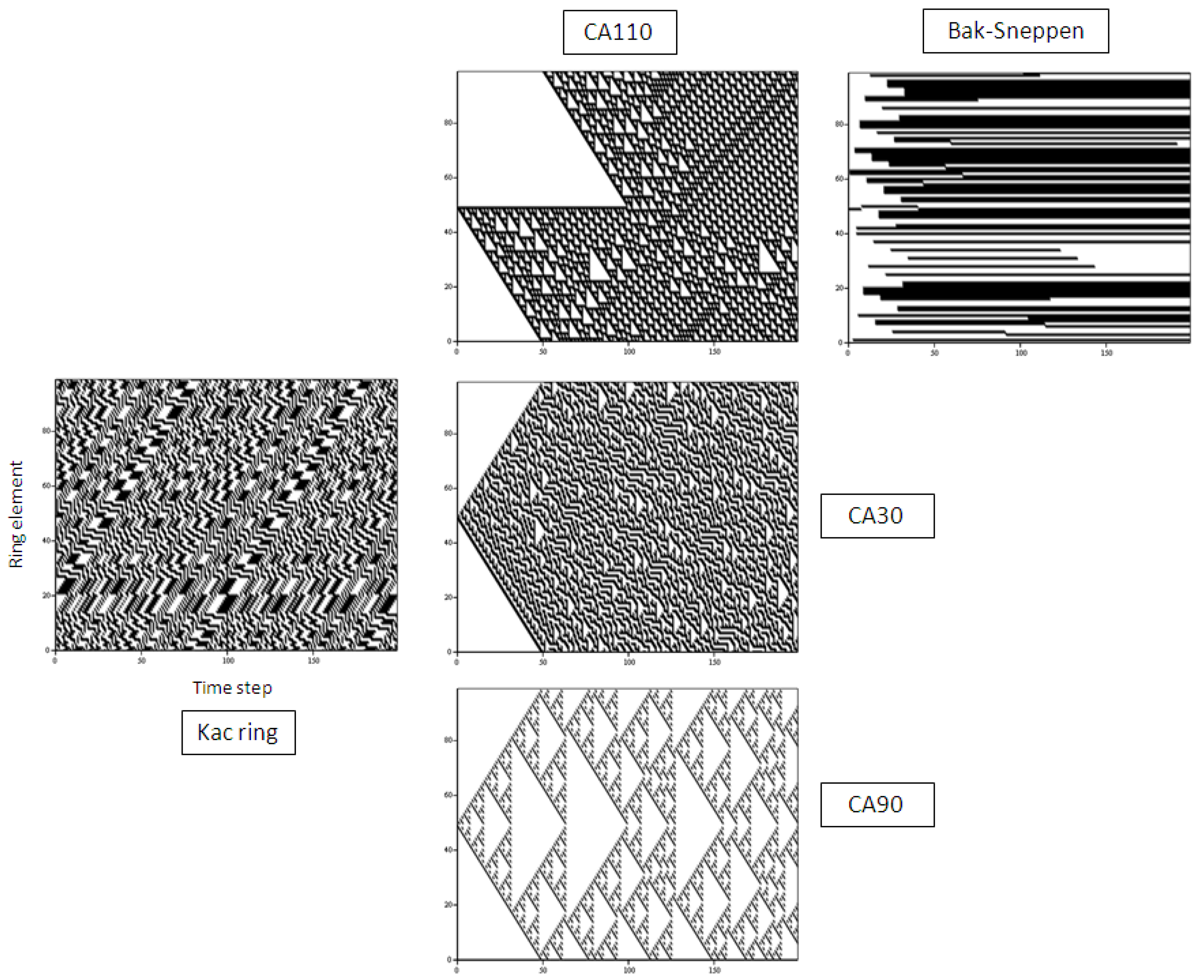
Figure 2.
Time steps 150 to 153 for all five rings in naturalistic representation.
2.5. A Note on Boolean Networks
It could be argued that the third large class of complex models, besides those aimed at producing self-organized criticality and cellular automata, are Boolean networks. These have featured prominently in the work of Stuart Kauffman and his evolutionary theory of complexity [23,24]. In a Boolean network, each node is connected to k other nodes by one of the following Boolean functions: AND, OR, TRUE, FALSE and potentially a set of non-exclusive variations. The state of is then determined by this function from the k input values of the connected nodes. In random Boolean networks the functions are assigned randomly to the sites.
For my ring with nearest-neighbour dynamics and two states of black or white, the minimum set of functions translates into the rule set summarized in Table 2. However, I was not able to obtain complex phenomenologies for this simple one-dimensional set-up. Figure 3b shows a typical result for a ring where each site carries a randomly assigned exclusive Boolean function fed by its two nearest-neighbours (Figure 3a). As displayed in the figure, the system quickly settled onto a stationary state. This might simply be the result of the need (induced by the desire to preserve comparability with the models presented in Section 2.1 to Section 2.3) to use k = 2 and to prescribe nearest-neighbour interactions. The model also does not use the full range of Boolean functions available since we have restricted ourselves to exclusive ones. However, it is also consistent with a tendency observed by Bak, one of the designers of the original Bak-Sneppen model, when working with random Boolean networks (quoted in [25], pp. 126–127):
“The result was always the same. The model would converge either to the frozen phase or to the chaotic phase, and only if the parameter C [equivalent to k above] was tuned very carefully would we get interesting complex, critical behaviour. […] Despite Stu’s early enthusiastic claims, for instance in his book The Origins of Order, […] that they exhibit self-organized criticality, they simply don’t.”
Table 2.
Boolean networks minimum rule sets. The upper line shows the parent triplet (, , ), the resulting colouring for is given below. 1 denotes black and 0 denotes white.
| Parent triplet | 1 xn,t 1 | 1 xn,t 0 | 0 xn,t 1 | 0 xn,t 0 |
|---|---|---|---|---|
| AND | 1 | 0 | 0 | 0 |
| OR | 0 | 1 | 1 | 0 |
| TRUE | 1 | 1 | 1 | 1 |
| FALSE | 0 | 0 | 0 | 0 |
Since it appears that including a Boolean ring as displayed in Figure 3 into my ensemble of models would not add much to either the discussion of dynamics or phenomenology, I have refrained from doing so.
Figure 3.
Boolean ring model. (a) Distribution of Boolean functions around the ring (red: AND; green: OR; blue: TRUE; black: FALSE); (b) Space-time diagram.
Figure 3.
Boolean ring model. (a) Distribution of Boolean functions around the ring (red: AND; green: OR; blue: TRUE; black: FALSE); (b) Space-time diagram.

3. Dynamical Properties of Complex Systems
In this section I will discuss the defining dynamical properties of complex systems. I will maintain a focus on differentiating complexity from pseudo-randomness, randomness and chaos. Whenever possible, I will refer back to our set of sample models for “verification”.
3.1. Complex Systems are Many-Component Systems
The concepts and terminology used in complexity science can be traced back to two genealogical roots: statistical mechanics and the study of simple computational systems, including chaos theory (e.g., [26]). The complexity encountered in the former, older field seems to agree closely with the Oxford dictionary definition of complexity as “the state or quality of being intricate or complicated”. Brownian motion [27], for example, appears intractable simply because there are so many particles interacting with each other that it becomes impossible for the human observer to account for them all. The systems studied in statistical mechanics were also among the first in which scale-dependent levels of descriptions were discovered. Once translated via probabilistic measures and coarse-graining to the macroscopic level, the random interactions of the micro-constituents can be captured by macroscopic variables with much simpler time developments. In an early discussion of complexity in science, Weaver [28] described the complexity of random systems in the following way:
“From this illustration it is clear what is meant by a problem of disorganized complexity. It is a problem in which the number of variables is very large, and one in which each of the many variables has a behavior which is individually erratic, or perhaps totally unknown. However, in spite of this helter-skelter, or unknown, behavior of all the individual variables, the system as a whole possesses certain orderly and analyzable average properties.”(p. 539)
Cellular automata, boolean networks and models of self-organized criticality, which are the categories under which the vast majority of systems traditionally studied in complexity can be grouped, are all models of the interaction of many constituents (e.g., for review, [7,22,24]). The two complex models discussed here each involve 100 cells interacting with each other—and are thereby at the lower end of the expected size for such simulations.
Given that all five of the studied systems are many-component systems of a similar characteristic size, this is clearly not a good criterion to demarcate the two complex systems from the random Kac ring, the pseudo-random CA30 or the regular CA90.
3.2. Complex Systems Feature Directed Interactions
Comparing the dynamics in an ensemble of particles in Brownian motion with those of the CA110 (Section 2.2) or the Bak-Sneppen model (Section 2.3), another important difference becomes apparent: in complex models constituents are linked by directed interactions. “Directed” here means that a constituent only interacts with a certain set of specific other constituents (e.g., in the models studied here, its nearest neighbours). To my knowledge, all of the other models denoted as complex also possess this property (e.g., for review, [7,22,24]).
In contrast, in the Kac ring model all particles have the same probability μ to experience a colour change (Section 2.1). Despite the fact that two sites might be placed next to each other on the ring, they are not linked in any way. Whether a particle will change colour is determined by an external quality, the edge markers. Similarly, in the random walk idealization of Brownian motion each particle’s likelihood to experience a collision is not dependent on the behaviour of a specific group of other particles. The existence of directed interactions is therefore a criterion that successfully distinguishes complex models from random ones, like the Kac ring.
3.3. Difference Between Complex and Chaotic Dynamics
The two dynamical properties discussed above are sufficient to distinguish complex systems from the mappings studied in chaos theory. The definition of chaos itself is not yet fully settled; however, it seem well established that non-linearity in chaotic mappings exclusively arises from self-feedback in a single, recurrent scalar or vector function (e.g., [29,30,31]). Considering a smattering of prominent examples illustrates this impressively: the chaotic pendulum, the Smale horse shoe map, the Hennon map and the logistic equation all fit this description. Chaotic mappings therefore need not be systems with a large number of constituents or directed interactions. Hilborn [30] has stated this distinction in the following way:
“To be somewhat more technical, we could say that these complex systems have many degrees of freedom, and it is the activity of these many degrees of freedom that leads to the apparently random behaviour. […] The crucial importance of chaos is that it provides an alternative explanation for this apparent randomness—one that depends neither on noise nor on complexity. Chaotic behaviour shows up in systems that are essentially free from noise and are also relatively simple—only a few degrees of freedom are active.”(p. 8)
While not all chaos theorists might subscribe to Hilborn’s [30] strong commitment to simple mappings, the formalism of chaos theory has been developed to deal predominantly with systems with few interacting variables (e.g., [29,30]).
While attempts have been made to translate the dynamics of the Wolfram CAs into differential equations [32] and to map differential equations into Boolean networks [24], none of these have been successful in establishing complete correspondence. Translating the probabilistic dynamics of the Bak-Sneppen model into any equivalent deterministic mapping appears to be even more difficult. Works on the relation between chaotic and probabilistic models so far have been mostly foundational and does not contain any pointers as to how multi-component interactions should be represented (e.g., [33]). The dynamics of complex and chaotic models in general are therefore fundamentally different.
Given that chaotic mapping and complex systems can relatively easily be differentiated from each other by dynamical criteria, it is somewhat surprising that the relationship between chaos and complexity has been such a convoluted one (e.g., [8]). Many complexity researchers seem to unquestioningly include chaotic systems under the umbrella of complexity. For example, Davies [34] states that “among the earliest complex systems to be studied were those we now refer to as chaotic” (p. 25). Similarly, Crutchfield and Young [35] developed the measure of statistical complexity for the logistic equation and Crutchfield [36] studied CA110 alongside this mapping.
Those who wish to differentiate between chaos and complexity have usually maintained that chaotic systems necessarily show sensitivity to initial conditions while complex systems need not do so (e.g., [7,37]). However, proclaiming directed interactions as necessary for complex dynamics actually eradicates the need to refer to auxiliary properties of the systems.
There seem to be three primary reasons why a strong separation between chaos and complexity science has not been achieved yet. One is the tendency to carelessly use the term “chaotic” as a synonym to “random” and “pseudo-random”, which will be discussed further in Section 4. Secondly, there is a conflation of historical and sociological continuity with epistemological connections. Thirdly, there is a misleading similarity of the common representations of chaotic systems to multi-component ones.
The fields of complexity and chaos theory are clearly linked by the biographies of some of their main protagonists. A sizeable contingent of the early complexity community, including Doyne Farmer, James Crutchfield and Norman Packard, recruited itself from the “Dynamical Systems Collective” (e.g., [38], p. 241), a group of young physicists at the University of California who had been amongst the first to systematically explore and describe non-linear equations. Potentially due to this very fact, there are striking similarities in the way the research community depicts complex and chaotic systems. In particular, despite the fact that chaotic maps only have one dependent scalar or vector variable, often multiple copies of or features from these maps are plotted against time and a given parameter (e.g., [30]). The resulting diagrams bear a close resemblance to the space-time diagram of a many-component system and are often analysed by very similar means. However, this treatment masks three important facts: that there is no equivalent “space” dimension for a chaotic mapping; that the plotted copies of the map are independent of each other; and that their ordering and spacing on the parameter dimension is arbitrary.
3.4. Benefits of a Dynamical Complexity Definition
In the struggle to capture the phenomenological features of complexity, the dynamics of these systems have often been treated as an afterthought only. Surprisingly, this is strikingly revealed in the attempts to develop computational (algorithmic) measures of complexity.
The concept of algorithmic information content of a specific binary sequence was developed independently by Solomonoff [39], Kolmogorov [40] and Chaitlin [41,42]. The algorithmic information content of a given binary sequence s is defined as the (bit) size of the minimum-length program needed to compute s (e.g., [43]). In order to assure absolute minimality, is defined for the Universal Turing Machine, hence the subscript in . However, as a consequence of the insolubility of the halting-problem discovered by Turing [44], minimal programmes on the Universal Turing Machine cannot be be determined and so algorithmic information content measures are fundamentally incomputable (e.g., [45]).
In the context of complexity research a variety of associated measures have been devised, for example logical depth [46] and effective complexity [47]. Dealing with the underlying program to create complex output, at first sight these measures appear to be dynamical ones. However, all of these measures, including the ones specifically developed by complexity scientists, are based on a hypothetical minimum program and not on the actual dynamics of the given system. They are therefore disguised phenomenological measures, which completely bypass the actual program, or rule set, that nature or our computer used to create the analysed binary sequences. The fact that the complexity community chose to base a large set of definitions on hypothetical, incomputable dynamics, rather than those actual occurring in complex systems, seems to indicate that the later were judged to be of little importance.
Another symptom of this dismissal is the prevalence of parsing studies, of which the best known ones were conducted by Wolfram [7] and Langton [48]. Instead of constructing dynamics from nature, these studies use the brute force approach of running large numbers of models based on variations of the same rule set. The models to be further investigated are then selected according to phenomenological criteria and any further discussion of their relation to real-life phenomena is based on the output as well (e.g., [7]). In contrast to traditional computer modelling, where the majority of creative work goes into designing models that provide a good or at the very least justified representation of nature (e.g., for review, [49]), the dynamics in these studies have no such specific meanings and are generated algorithmically.
However, based on the review in this section, I maintain that the complexity definitions developed above are not only essential in differentiating complexity from random and chaotic systems, but that they could also act as guide towards those aspects of complexity that are unique and warrant special academic attention. Conclusive evidence for the prevalence of complexity in nature cannot be obtained by a mere comparison of phenomenological features: instead, complexity research should aim to identify and categorise the occurrence of complex dynamics, focusing on directed, many-component interactions. Similarly, recognizing that complexity is related to unique dynamic properties also provides a firmer basis for the development of complexity measures. As I will show in Section 4, phenomenological complexity measures alone are not sufficient to differentiate complexity from pseudo-randomness. A more productive way forward could be the development of complexity measures that implicitly refer to the two dynamical criteria outlined in Section 3.1 and Section 3.2.
4. Phenomenological Properties of Complex Systems
In this section I will discuss the phenomenological properties of complex systems and extend our complexity definition to include a phenomenological sieve, distinguishing those models we want to denote as “complex” from others with similar dynamics. I will also review previous attempts at defining complexity phenomenological and will note that the descriptive metaphors abounding in the field often indicate the presence of dynamic or naturalistic properties of complexity for which there is little or no justification. I will show that quantitative measures based on these metaphors do not reliably distinguish complex phenomenons from random and pseudo-random ones.
4.1. The Need for a Phenomenological Sieve
We have seen in Section 3 that a suitable dynamical definition can be found which already accomplishes the aim expressed in this paper’s title: it disentangles complexity from randomness and chaos. However, it does not guarantee that every many-component system with directed interactions will produce output that should be described as complex. In fact, a glance at Figure 1 shows that two of the Wolfram CAs in my sample produce space-time diagrams which can be adequately described by existing terminology: the CA30 appears “pseudo-random” and the CA90 shows a “nested, regular structure”. It is only the CA110 whose representation does not appear to be adequately captured by either of these terms.
It would be fair to say that, in the history of complexity science, the assumption that humans generally perceive the space-time diagram of CA110 and the Bak-Sneppen model as different from those of CA30 and CA90 constitutes the single most important statement. Complexity scientists are fond of relating “their discovery” of complexity with the same pathos that particle scientists employ when describing the discovery of a new quark (e.g., [7,26]). To my knowledge, this proposition has never been explicitly tested, i.e., there exists no longitudinal studies of whether “complex” phase space diagrams are reliably recognized as distinct. However, for the purpose of this paper I will assume that there is a universally recognizable difference between the space-time diagrams of the two complex models and our remaining three simulations. Most existing complexity definitions aim to go beyond this basic assertion and to provide a qualitative description of complexity. In the following sections I will consider several pertinent problems in trying to specify complexity thus.
4.2. Where Does Complexity Manifest Itself?
It is important to realise that complexity science’s phenomenological discussions refer very specifically to patterns recognized in the models’ computer output. This often requires considerable restructuring of the data, so that the images shown for illustration might create the illusion of a spatial pattern in physical space, while in reality it lies in one or more abstract dimensions. For example, Figure 1 plots the values of one-dimensional models versus time, creating two-dimensional pictures. Each row is thereby the state of the automaton at a different iteration. The patterns we recognize are clearly two dimensional ones: nested triangles, patches and stripes. In a naturalistic correct, one-dimensional representation of the row of cells that constitute the system, these would manifest as fluctuations without an obvious geometrical counterpart. This is illustrated in Figure 2, which shows short sequences of the development of the models in their natural representations. Despite the fact that I have chosen my set of models so that all of them can be presented as two coloured rings, and thus ensured comparability, the patterns that are clearly different in the space-time diagrams are not as easily detectable in this representation.
This can be verified even better by watching the animations of the full runs collected in Appendix A of this paper. While the regularities in the CA90 automaton quickly become obvious, the four other rings display virtually indistinguishable disordered flickering of colours. Individuals’ pattern perception might vary greatly and only careful psychological testing would be able to conclusively decide this point, but it seems apparent that complexity is much less recognizable in the naturalistic representation than it is in the space-time diagram.
The importance of data analysis for the definition of complexity was recognized in an early discussion of the topic by Rosen [50]:
“We are going to define a complex system as one with which we can interact effectively in many different kinds of ways, each requiring a different mode of system description.”(p. 29)
In modern complexity science, the dimensionality of the representations analysed seems to be regarded as mostly unimportant. This has already become evident in Section 3.3, where I discussed the fact that plots of chaotic functions in parameter space are often directly compared with complex space-time diagrams. It is also apparent in the manner in which the claim for the prevalence of complexity in nature is frequently justified: by identifying the patterns seen in a model’s space-time diagram as if they were in physical space. Numerous examples of this practice can be found in Wolfram [7], who compares images similar to those displayed in Figure 1 to snowflakes, rock fault lines, leaf arrangements and a variety of other two-dimensional physical patterns. At the same time, for many of these examples virtually no attempts are made to translate the process of creation that is associated with the space-time patterns (e.g., production and adjunction of a slightly altered version of itself, according to certain rules) into a mechanism that could operate in physical space. This holds true for similar comparisons with higher-dimensional models as well. Disregarding the consequences that could be drawn from this observation for future research programs in complexity science, the discussion in this section indicates that our eventual phenomenological sieve will have to be defined in a representation dependent way.
4.3. How Can Complexity be Described?
Of course, merely recognizing that some many-component systems with directed interactions (in some representations) can be visually differentiated from pseudo-randomness and regularity is scientifically unsatisfactory. Such a restricted definition neither allows us to specify how complexity relates to the two established categories, nor does it lead to a quantitative assessment of complexity. For example, this basic description would make it impossible for us to decide whether the CA110 or the Bak-Sneppen model is more complex.
However, casting the qualitative nature of complexity into words has been proven difficult. As indicated in the introduction and by the motto I have chosen for this paper, I view a lack of openly recognizing this difficulty, and instead hiding it behind a mirage of picturesque phrases, as one of the major problems of complexity science. It is the continuous existence of a number of fuzzy concepts at the very core of complexity science that rightly provokes criticism like the one by Horgan [8].
A review of previous phenomenological complexity definitions shows that they suffer from two prime faults: either the description is semantically circular and adds little to the already established restricted definition; or it is overly metaphorical and implies scientific relationships for which there is little evidence. I will use these two categories—semantic singularity and metaphorical over-reach—to structure our review and critique of the most popular complexity definitions.
4.3.1. Semantic Circularity
Wolfram [16] made an early attempt to formalize the intuitive notions of visually detectable complexity for cellular automata like the ones discussed in Section 2.2. He introduced the following “classes of behaviour”:
“Class 1—evolution leads to a homogeneous state in which, for example, all sites have value 0.Class 2—evolution leads to a set of stable or periodic solutions that are separated and simple.Class 3—evolution leads to a chaotic pattern.Class 4—evolution leads to complex structures, sometimes long-lived.”(p. 9)
The term “chaotic” is used here to imply “pseudo-random” (Section 3.3). Neither here nor in any of the author’s later works reiterating this classification scheme [7,17,18,19,51] is any definition of the term “complex” given. The connotation attached to it is markedly different from the one used in Wolfram [15], where a large number of nested, and therefore Class 2, cellular automata are advertised as “complex”. However, viewed in combination with the other three categories, the Class 4 automata are classified as “complex” simply because they fit into none of the other categories. This, of course, relies on the fundamental assertion that we can perceptually detect complexity discussed in Section 4.1. There is no positive identification for complexity in this scheme—altogether one is left with the feeling that “complex” is meant to be seen as an intuitively understood description.
However, Wolfram [17]’s later articulation of the scheme added one additional characteristic: he defines the class 4 automata as “complicated, localised structures, some propagating” (p. 5). While “complicated” is used interchangeably with “complex” and does not add to the definition, localisation is clearly a novel qualitative concept and one that is more apparent in the CA110 and Bak-Sneppen model than in any of the other models (Figure 1). In Section 5, I will return to this idea.
In keeping with the circularity displayed in his categorisation scheme, Wolfram has been adamantly claiming that complexity will be obvious to the beholder and that no formal definition is necessary. Asked by Gershenson [52] about a definition of complexity, he states that a formal definition “tends not to be particularly critical” and that:
“[T]he intuitive notion is fairly clear: things seem complex if we don’t have a simple way to describe them.”(p. 131)
However, as outlined in the previous sections of this paper, I believe that while it is certainly prudent to be conservative about verbalising a phenomenological complexity definition, there are many unexplored but promising avenues through which one could approach the task.
4.3.2. Metaphorical Over-Reach
Other phenomenological definitions of complexity have tried to move beyond the assumption that complexity is just “different” and explicitly include a positioning of complexity with respect to randomness/pseudo-randomness (or chaos) and regularity. These often rely on metaphorical descriptions. I will discuss the most popular qualitative descriptions and their associated quantitative measures below. In particular, I will first describe and test the validity of the metaphor of “complexity between order and disorder”, including the associated concept of “the edge of chaos”. Secondly, I will deal with the idea of “self-organisation”, which is another key term in complexity science. It will become apparent in my review that all three of these metaphors are lacking scientific grounding.
4.3.2.1. Complexity Between Order and Disorder
The most successful and widespread of these metaphors is the description of complexity being located between order and disorder (e.g., for review, [53,54]). Even Wolfram [7] includes this image in the latest version of his classification scheme:
“And finally [] class 4 involves a mixture of order and randomness: localised structures are produced which on their own are fairly simple, but these structures move around and interact with each other in very complicated ways.”(p. 235)
An advantage of this description is that it can be easily used to create predictions for quantitative complexity measures. The traditional measure for disorder is entropy, which assigns maximum values to random phase space distributions and minimum values to regular ones (e.g., [55,56]). If the phenomenology of complex systems can be adequately described as between order and disorder, then an analysis of their outputs should yield medium entropy values. A second class of complexity measures has been defined by rescalings of the traditional entropy in such a way that both a pseudo-random as well as a regular phase space distribution will yield minimum complexity values (e.g., [53,57]). These measures are expected to yield maximum values for complex systems, which, according to the metaphor, should fall somewhere between the two minima.
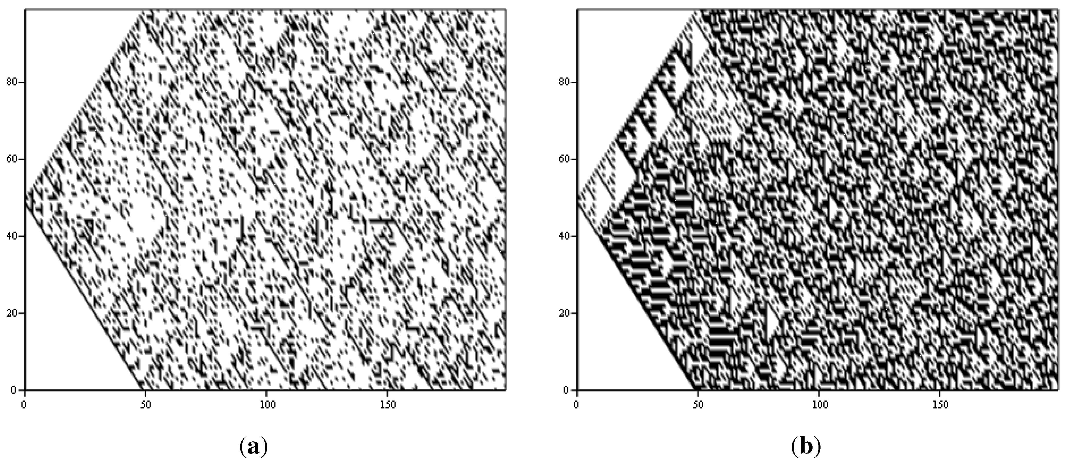
How accurate is the phenomenological description of complexity as located between order and disorder? Comparing the two complex space time-diagrams in Figure 1 to the disordered (Kac ring and CA30) and the regular (CA90) ones does not indicate that the patterns in the complex output are produced by direct superposition, or as a “mixture” of ordered and disordered patterns. I have tested this explicitly by producing superpositions of the CA30 and CA90 space-time diagrams (Figure 1), an example of which is shown in Figure 4a. Thereby, a new space-time diagram is constructed by choosing each point from either the CA30 or the CA90 diagram with a given probability. Figure 4a mixes 70 percent of the regular CA90 with 30 percent of the pseudo-random CA30 and represents my best attempt at creating complexity in this naive way. As can be seen easily by comparison to the space-time diagrams of CA110 or the Bak-Sneppen model in Figure 1, it is clearly not successful. Similarly, coupling the dynamics of CA90 and CA30 fails to produce complex phenomenologies. Figure 4b shows the space-time diagram obtained for a coupled cellular automaton in which, during each time step, a cell is updated according to the CA30 rule set (Table 1) with 5 percent probability or according to the CA90 rules (Table 1) with 95 percent probability. The space-time diagram shown is again the “best” result of a scan through the parameter space of possible probabilities. The resulting space-time diagram only vaguely resembles the complex phenomenologies in the very early stages of the simulation. While the coupling studies are crude, they do indicate that a naive interpretation of the “complexity between order and disorder” metaphor is not correct.
Figure 4.
Direct combinations of CA90 and CA30. (a) Superposition of the space-time diagrams (Figure 1) with probabilities of 0.3 (CA30) and 0.7 (CA90); (b) Space-time diagram for coupling with probabilities 0.05 (CA30) and 0.95 (CA90).
Figure 4.
Direct combinations of CA90 and CA30. (a) Superposition of the space-time diagrams (Figure 1) with probabilities of 0.3 (CA30) and 0.7 (CA90); (b) Space-time diagram for coupling with probabilities 0.05 (CA30) and 0.95 (CA90).
Instead, in the complex space-time diagrams (Figure 1) there seem to be localised regions with potentially different degrees of order. In the CA110 output, a relatively (but not completely) regular pattern of diagonally running stripes coexists with veins of apparently disorderly distributed small scale triangles. Similarly, the Bak-Sneppen model produces a (relatively) regular stripe pattern that is occasionally broken by irregular patches of solid colour. However, it seems that the different localised patterns present in the complex space-time diagrams tend to one of the two extremes, so that the a description of complexity as “between order and disorder” is not fully correct. It also implies that, especially since in both cases we have on average an approximately equal distribution of black and white balls (also compare Figure 2), the quantitative measures discussed above will most likely not be able to clearly distinguish complexity from randomness.
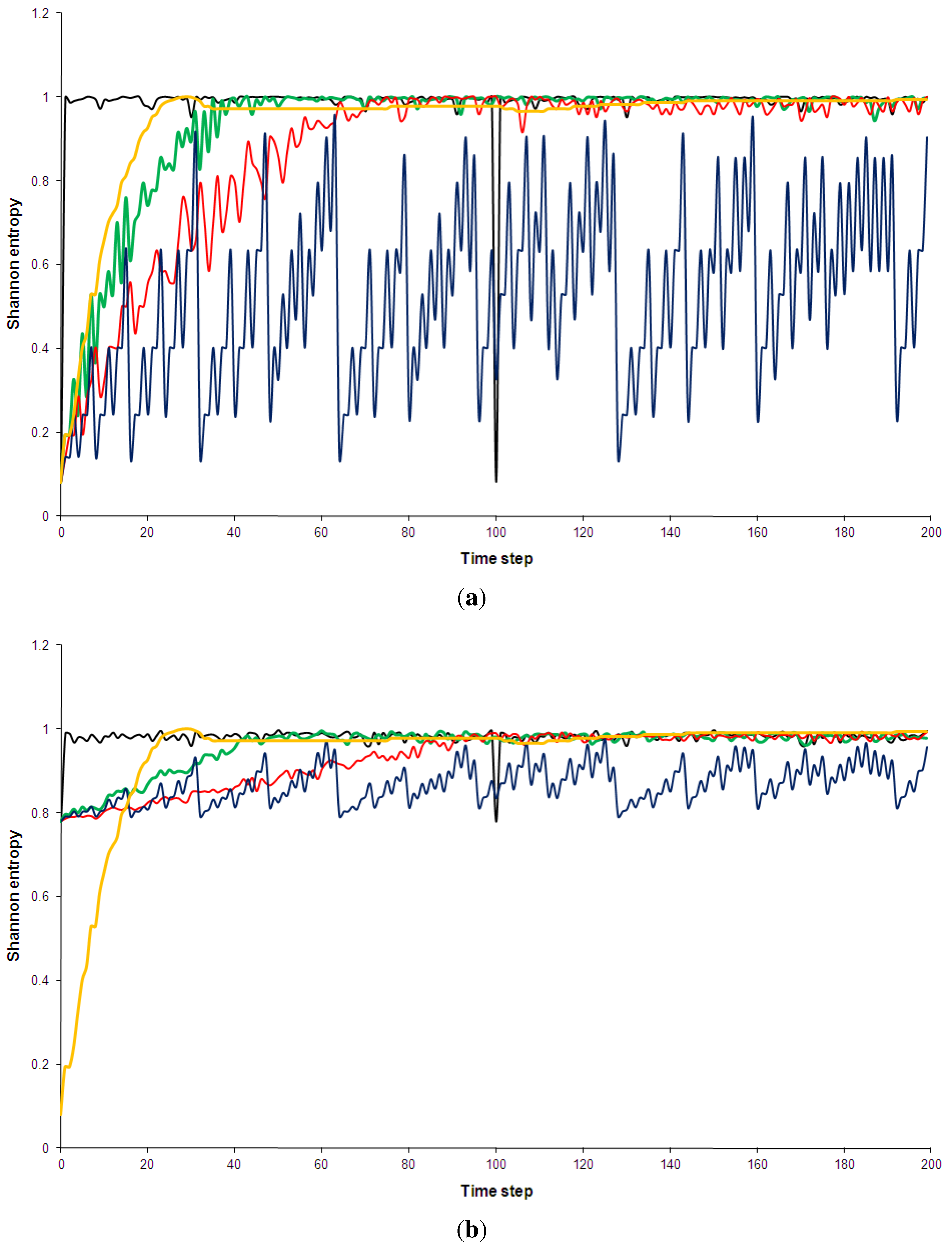
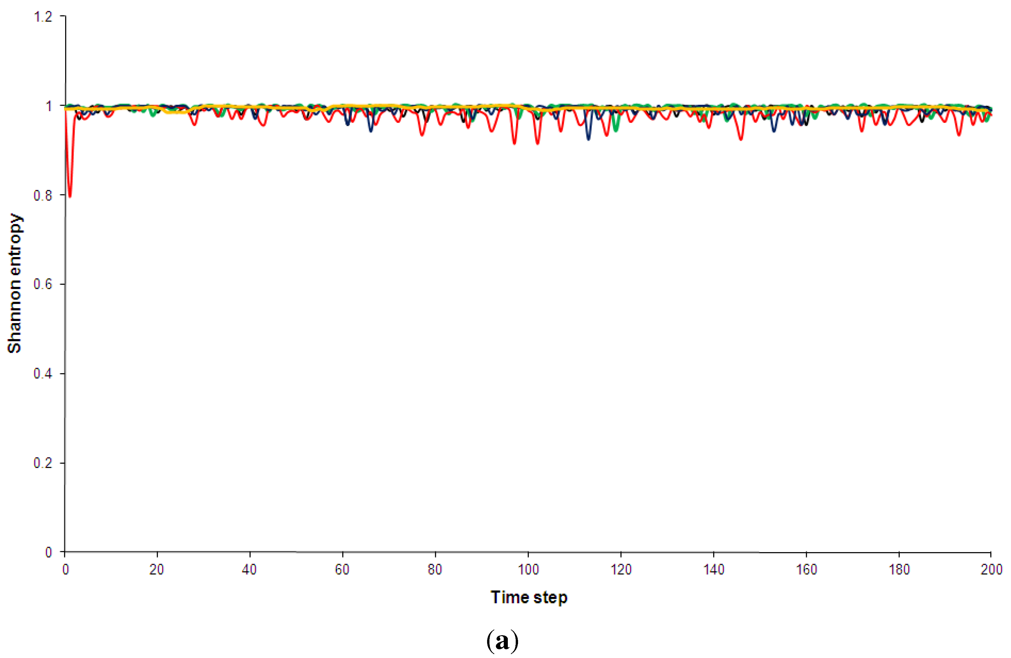
This observation is borne out in Figure 5 and Figure 6, which show comparisons of the time development of the Shannon entropy and the (simplified) statistical complexity for all five models analysed here. Some technical details of the measures and full explanations of my calculations are given in Appendix B, Appendix C and Appendix D of this paper.
Figure 5.
Shannon entropy of the five models discussed in Section 2. Black: Kac ring. Green: CA30. Blue: CA90. Red: CA110. Yellow: Bak-Sneppen model. In (a) the entropy for no spatial partitions of the ring is shown while in (b) the partition included 10 spatial segments (see Appendix D for details).

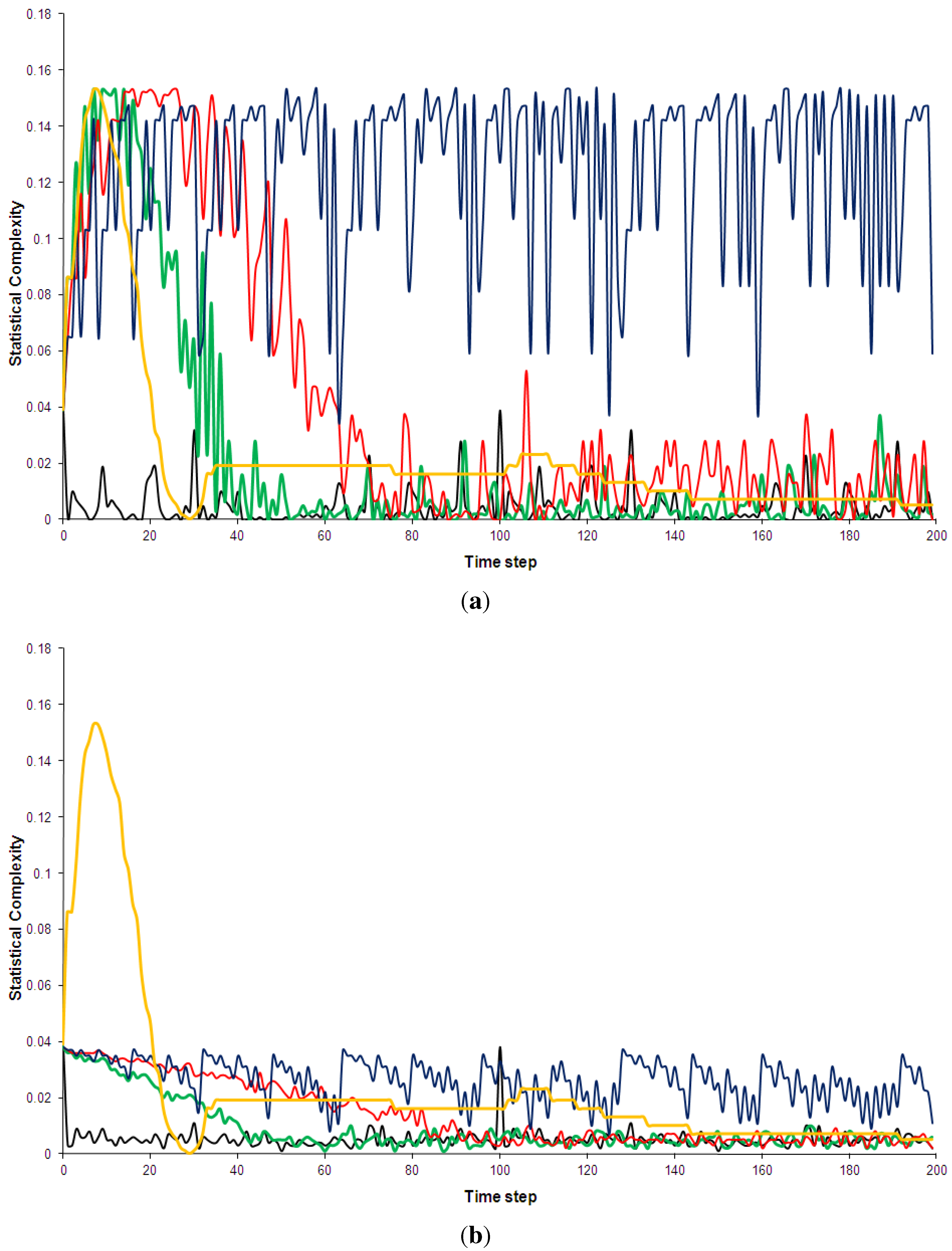
Figure 6.
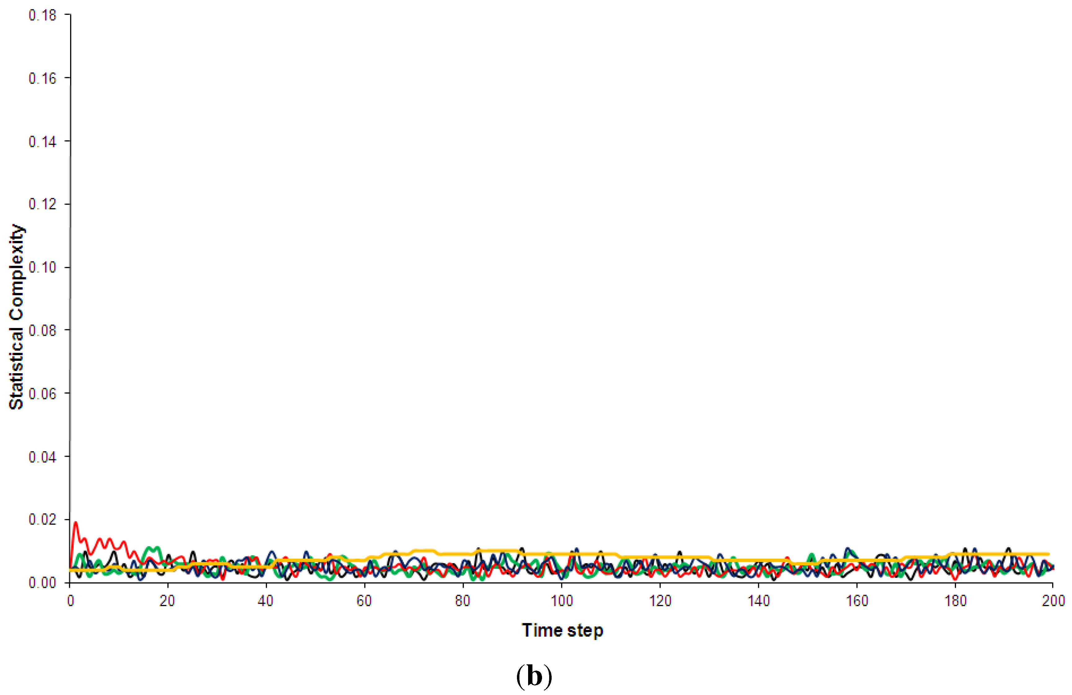
Statistical complexity of the five models discussed in Section 2. Black: Kac ring. Green: CA30. Blue: CA90. Red: CA110. Yellow: Bak-Sneppen model. In (a) the entropy for no spatial partitions of the ring is shown while in (b) the partition included 10 spatial segments (see Appendix D for details).
Figure 6.
Statistical complexity of the five models discussed in Section 2. Black: Kac ring. Green: CA30. Blue: CA90. Red: CA110. Yellow: Bak-Sneppen model. In (a) the entropy for no spatial partitions of the ring is shown while in (b) the partition included 10 spatial segments (see Appendix D for details).

Shannon entropy has been chosen over Boltzmann’s traditional entropy since it is normalized (for a review of different entropy measures, e.g., [56]). As can be see in Figure 5, the pseudo-random, random and the complex models quickly approach maximum entropy states. This is true even when a spatial partition of 10 segments is used (additional computations not shown here indicated that this result is independent of the spatial partition used). The use of a spatial partition makes the entropy more sensitive to certain mesoscale structures, e.g., it would give low entropy if many solidly coloured segments were present. The technical details of partitioning phase spaces for the entropy and complexity calculations are discussed in Appendix D. The regular CA90 is clearly visible in the entropy diagram: it is distinguished not so much by consistently low entropy but by regular entropy fluctuations. However, once the runs have settled, the average entropy values for the complex systems are not hugely different from the random and pseudo-random ones (Table 3). Similarly, none of the complex models shows an overall trend of decreasing entropy, as has been predicted by supporters of the “complexity between order and disorder” metaphor (e.g., for a review of this claim, [37]).
Table 3.
Average entropy and complexity values for the last 100 time steps of the five models. Partition 1 is the partition without spatial cells and Partition 2 is a partition with 10 spatial segments.
| Entropy | Complexity | |||
|---|---|---|---|---|
| Partition 1 | Partition 2 | Partition 1 | Partition 2 | |
| Kac ring | 0.985 | 0.980 | 0.00463 | 0.0053 |
| CA30 | 0.993 | 0.982 | 0.00475 | 0.00493 |
| CA110 | 0.980 | 0.982 | 0.0136 | 0.00505 |
| Bak-Sneppen | 0.984 | 0.972 | 0.0106 | 0.00762 |
| CA90 | 0.587 | 0.885 | 0.126 | 0.0240 |
I am using the simplified statistical complexity [58] which is an adapted version of the measure developed by Crutchfield and Young [35]. The statistical complexity assigns minimum values to both disordered as well as ordered states and has therefore been endorsed by Ladyman et al. [53] as “illustrative of a good measure of complexity” (p. 31). However, the most frequent application of this measure has been to the logistic equation [35,36,57,58,59] and, to our knowledge, there exists no comparative studies of complex and non-complex models. These are clearly the type of studies in which quantitative complexity measures will have to prove their worth.
In Figure 6 the statistical complexity values for the five models are plotted. The Kac ring and CA90 both have low complexity values, as expected for random and pseudo-random phenomenologies. The regular model is again clearly distinguished from the other four by large fluctuations and a generally higher complexity. Given that the statistical complexity was designed so that low values should be assigned to ordered sequences, this is a somewhat surprising result. In addition, this measure also fails to clearly pick out the complex models, which are also given relative low values. After a short initial “spin-up” period the statistical complexity of CA110 is only marginally higher than that of the Kac-ring or CA30 (Table 3 and Figure 6). The Bak-Sneppen model fares somewhat better and even experiences a short intermittent period of increasing complexity, but the overall trend is towards a decrease in complexity as the run progresses. After 160 time steps the complexity profiles of the complex and the random/pseudo-random models are virtually indistinguishable. This is true for all spatial partitions used (e.g., Figure 6b).
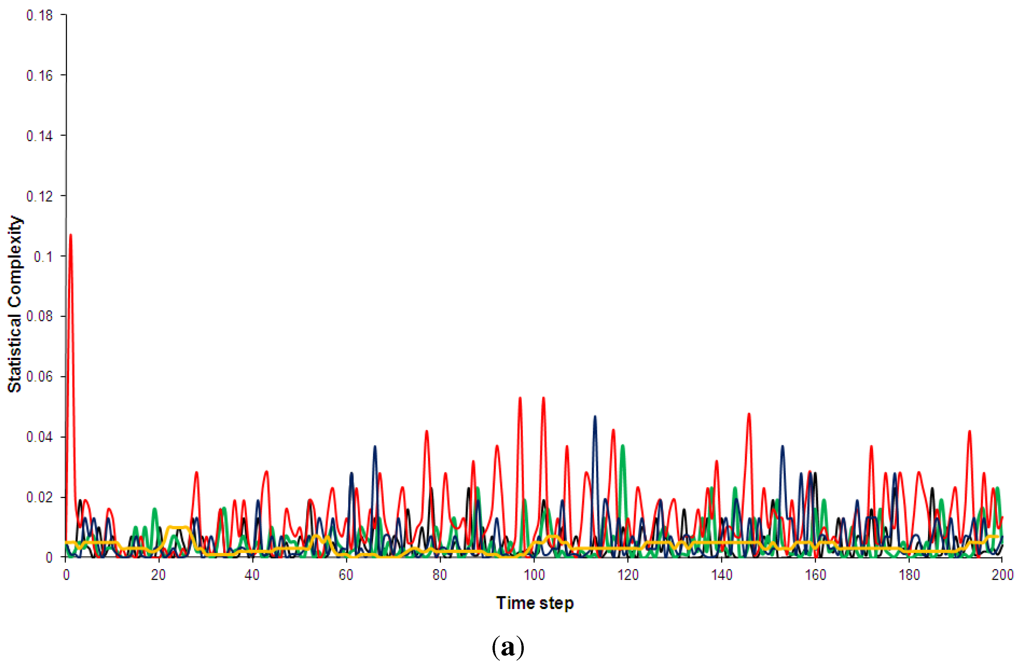
In comparative study such as this, the statistical measures based on the metaphor cannot be judged successful in distinguishing between complexity and pseudo-randomness/randomness. They also provide no meaningful quantitative ranking of the complex models tested. This seems to be due to the fact that each of the localised, differently patterned regions composing the complex models’ space-time diagrams individually have high entropy and low complexity, i.e., they have a relatively even spread through a phase space consisting of the two colours and, if a spatial partition is used, the positions on the ring. It should be noted that I have started the simulations from an initial sate that maximizes differences in the phenomenology. Appendix E contains results from runs started from a random initial state. The entropy and complexity values for the five models are even less distinguishable in this case.
Atmanspacher et al. [60] have argued that traditional complexity measures are too simplistic to adequately describe complex models:
“In general, their analysis has to be a meta-analysis, and in general it has to be based on meta-statistics instead of conventional first-order statistics.”(p. 828)
The block entropy devised by Wolfram [7,17], mutual entropy [43] or the original version of the statistical complexity by Crutchfield [36]—which all aim to calculate entropies based on the occurrence of sub-sequences rather than simple phase space spread—might constitute such meta-statistical measures. However, unless huge computational resources are to be mobilised for each entropy computation, the measures will have to rely on the heuristics of human perception to pick out sub-sequences that are apparent in the space-time diagrams and can be parameterized in a search algorithm. These could be, for example, the stripes and solid regions in the Bak-Sneppen model, or the diagonally stacked small scale and pseudo-randomly distributed mesoscale triangles for the CA110. However, even such meta-statistics would still assign higher complexity values to the regular CA90. which is composed of a larger number of regular sequences. This, and the computational expense, might be the reason that very few studies of actual complex models, and no comparative investigations, have been undertaken with these measures.
4.3.2.2. Complexity at the Edge of Chaos
The description of complexity between order and disorder has spawned another popular phrase: complexity as located “at the edge of chaos”. Langton [48] introduced a concept called the λ-parameterisation of the CA rule space. Thereby rules which heavily favour one particular transition state (called the quiescent state) are assigned low λ values, while high values of λ indicate that very few configurations of CA will lead to . He found that class IV behaviour is displayed by CAs with rule sets characterised by medium λ values. For high λ values one obtains class III (pseudo-random) behaviour, for low ones the phase space outputs were ordered (class I) or periodic (class II). A further discovery of Langton [48]’s scan through the parameterized rule space was the fact that the transition from ordered to disordered regime appears to be sudden rather than gradual. In analogy to the phenomenon in thermal physics, this has been named a “phase transition” [48] (p. 24). The realisation that the complex CAs occupy only the small region of rule parameter space right before the order-disorder transition occurs fits with the earlier hypothesis that the class IV set of rules should have zero measure [61]. This parameter space location of the class IV automata inspired the influential phrase of complexity being located at the “edge of chaos” (e.g., [48], p. 36).
Langton [48]’s experiments have not been unequivocally replicated and it is therefore debated whether the transition between the CA behaviour classes really exists [62]. Interviewed by Coveney [10], Mitchell, a colleague of Langton’s at the Santa Fe Institut, passes a damning verdict on both the metaphor and the study:
“To the extent that one can make sense of what Packard and Langton meant by “the edge of chaos”, their interpretation of their simulation results are neither adequately supported nor are they correct on mathematical grounds.”(p. 276)
However, the phrase itself has become wide-spread and features in all of the popular books on complexity (e.g., [3,23,26]).
As I have shown in Section 3.3, chaotic systems are dynamically distinct from complex ones and Langton [48]’s cellular automata were clearly not transitioning to a chaotic phenomenology but to a pseudo-random one. “Complexity at the edge of pseudo-randomness” does not have as much of poetic ring to it but would probably have lead to an earlier severing of the (we think) unhelpful ties to chaos theory. The metaphor has both prolonged the widespread use of “chaotic” as interchangeable with “disordered” and directly led to the development of some complexity measures on chaotic mappings (Section 4.3.2.1). In fact, the fast majority of actual quantitative complexity calculations seem to have been carried out for the logistic equation [35,36,57,58,59]—often specifically in search for the “edge of chaos”—and therefore provide little indication for the behaviour of the complex systems studied here.
Outside the context of genetic algorithms, it is difficult to relate the phrase (which was after all defined during a dynamical investigation) to phenomenologies like the ones displayed in Figure 1 and Figure 2. Kauffmann [23] contains the following illustration of “the edge of chaos”-type behaviour in the naturalistic representation of a field of inter-connected light bulbs:
“But at the edge of chaos, the twinkling unfrozen islands are in tendrils of contact. Flipping any single lightbulb may send signals in small or large cascades of changes across the systems to distant sites, so the behaviours in time and across the webbed network might become coordinated. Yet since the system is at the edge of chaos, but not actually chaotic, the system will not veer into uncoordinated twitching”(p. 90)
However, our previous attempts at qualitatively describing both naturalistic and space-time representations of complex systems illustrates that a more technical language use is required to devise a description that can be translated into a successful quantitative measure. Since the validity of the “edge of chaos” proposition is doubtful even in the narrow sub-field it was originally coined for and it has significantly furthered the false impression of a close connection between complexity and chaos, the popularity of this expression seems to have done more harm than good.
4.3.2.3. Self-Organized Complexity
In parallel to the metaphors based on the relation of complexity to order and disorder, another set of metaphorical descriptions inspired by biology and artificial life has been developed. These are related to the concept of “self-organisation” and use terms like “memory”, “co-ordination” and “self-organized criticality” to describe the phenomenology of complex models (e.g., [23,37,63]). The Bak-Sneppen model and its classical cousins were instrumental in introducing the term “self-organized” criticality, which crucially depends on “avalanches” (e.g., [64])—the appearance of episodes of short but intense change; in Figure 1 these are indicated by solid coloured areas in the model, in the continuous version they show up more impressively as multi-coloured patches. The size of these events can be related to their frequencies by a power law (e.g., [25]). Frigg [22] contains an expansive critique of generalist claims made for the occurrence of “self-organized criticality” in nature. I agree with his scepticism, however, my own focus here is not on the realism of the conceptual content of this sub-field of complexity science but on a mismatch between this content and the language used to describe it. Self-organized criticality and similar metaphors interpret phenomenological features like episodic turmoil as a crucial mechanism to adjust the overall state of the model. Ladyman et al. [53] even include a mention of “memory” into their general complexity definition (which I will discuss in detail in Section 5).
The most problematic aspect of these “self-organisation” metaphors is the suggestion of dynamical processes when they are actually describing phenomenology. “Memory” and “organisation” are meta-dynamical descriptions that should be inferred from the dynamics of the system (e.g., by considering the effects of directed interactions) rather than ascribed to a model’s output. The use of the terms again shows a tendency to construct retrospective virtual dynamics rather than to view the model as an entity in which the phenomenology is fundamentally linked to a given dynamics (Section 3). In the realm of science fiction this disconnection has given rise to the commercially successful idea of “swarm intelligence” [2]—however, science itself should not be at liberty to choose prose over factual accuracy.
Due to the fact that the “self-organization” metaphors have no dynamical counterparts, their epistemic usefulness appears to be very low. This sentiment is well illustrated by a statement from Francis Crick, made when interviewed by Coveney [10] about the importance of self-organisation during brain development:
When viewed as mere descriptions of phenomenology, it seems doubtful whether the “self-organisation” metaphors add much to the descriptions of diagrams like the ones displayed in Figure 1 and Figure 2. For example, the expression “memory”, with its connotation of temporal continuity, could be employed to describe the elongated structure of dense, meso-scale triangles in the CA110 space-time diagram. However, this seems to improve little to the geometric description given in the second part of the last sentences—and introduces the faulty dynamical connotations exposed above.“Who or what else is organizing it [the brain] if it is not doing it itself? There are a number of ways that the brain can self-organize. What we want to know is which way it does it.”(p. 285)
5. Conclusions
Following my brief review of previous attempts to qualitatively and quantitatively define complexity, I will now combine the results from Section 3 and Section 4. My major concern will be to avoid the semantic circularities while committing myself to a more austere linguistics standard than the existing metaphorical descriptions. I also wish to give due weight to the dynamical properties of complex systems, which are instrumental in distinguishing complexity from randomness and chaos.
Reflecting my view that recognition of phenomenological complexity is fundamentally a process of human perception, I will use the psychological term “pattern” to indicate the spatial structures seen in the complex space-time diagrams in Figure 1. Following Wolfram [7,17,18,19,51]’s definition, I will use the term “localised” to indicate that different regions of the diagram can be distinguished by their patterns. Lastly, Section 4.2 indicates that it will be prudent to include a pointer towards the representation dependency of phenomenological complexity. Combining these elements we add the following phenomenological sieve to our dynamical complexity definition:
Definition 1. A complex system is a many-component system with directed interactions for which locally distinct patterns can be recognized in at least one representation of its development.
My definition is successful in demarcating the models in my small sample set (Section 2): the Kac ring is weeded out by the dynamical criterion of directed interactions and the two “boring” CAs with global chaotic and regular patterns are kept back in the phenomenological sieve. More important than securing the verdict that the Kac ring is non-complex, which would also have been accomplished by the phenomenological part, the requirement of directed interactions also clearly renders all chaotic systems non-complex, independent of their phenomenologies. A cursory application of the definition to the models collected in Wolfram [7] shows that it will successfully describe those CAs which are commonly categorized into Class 4 (Section 4.3).
To see how my definition fares in comparison to other authors’ formal ones, I will consider the following example by Ladyman [53], who set out on a similar quest to mine and who end up proposing to define complexity in the following way:
“A complex system is an ensemble of many elements which are interacting in a disordered way, resulting in robust organisation and memory.”(p. 25)
Interaction in a disordered way is clearly a feature of random systems rather than of complex ones (Section 3.2). Further perusal of their article shows that this is in fact just a lapse in language and what they mean is a disordered phase-space distribution. “Robust organisation” and “memory” are taken from the stock of metaphors commonly used to described complexity. In keeping with the general trend discussed in Section 4, it remains unclear whether “organisation” and “memory” refer to phenomenological appearance or dynamical properties. The definition is neither precise enough in distinguishing between dynamics and phenomenology nor does it enforce enough clarity in the use of terminology to meaningfully set aside complexity from chaos or randomness.
Gershenson [52] made a collection of short interviews with influential complexity researchers. Asked in these questionnaires how they would define complexity, the large majority declines to offer a formal definition. However, I see several benefits in having made the effort to design Definition 1. Firstly, the process of clarifying the boundaries of a concept and disentangling it from its hereditary fields helps to eradicate unsuitable connotations and imprecise language. In my case, the most prominent victim of this pruning process is clearly the “edge of chaos”. Secondly, the definition itself acts as a guide towards the essential properties of the concept and those that warrant further investigation. These, in my opinion, are the definition and detection of patterns in the phenomenology as well as the influence of interconnection and interaction in multi-component systems. The latter dynamical aspect and its relation to nature should be examined without the influence of vague metaphors derived from the phenomenological description of the systems. Ideally, a future description of the phenomenologies of complex models should relate these directly to the underlying dynamics. This might utilize the existing large-scale parsing studies (e.g., [7,48])—or might start from completely new premises!
Acknowledgements
I am very grateful to Jeremy Butterfield for his help with this project. I also thank Nazim Bouatta, Katharina Kraus, Arianne Shavisi, Kirsten Lillie, Peter Gunstone and an unknown reviewer for their suggestions and help with the manuscript.
References
- Gell-Mann, M. The Quark and the Jaguar: Adventures in the Simple and the Complex; W. H. Freemann: New York, NY, USA, 1994. [Google Scholar]
- Schaetzing, F. The Swarm; Regan Books: New York, NY, USA, 2006. [Google Scholar]
- Mitchell, M. Complexity: A Guided Tour; Oxford University Press: Oxford, UK, 2009. [Google Scholar]
- Standish, R.K. Concept and Definition of Complexity. In Intelligent Complex Adaptive Systems; Yang, A., Shan, Y., Eds.; IGI Global: Hershey, PA, USA, 2008; pp. 105–124. [Google Scholar]
- Gell-Mann, M. What is complexity? Complexity 1995, 1, 1–9. [Google Scholar]
- Lloyd, S. Measures of complexity: A Nonexhaustive List. IEEE Control Syst. Mag. 2001, 21, 7–8. [Google Scholar] [CrossRef]
- Wolfram, S. A New Kind of Science; Wolfram Media: Champaign, IL, USA, 2002. [Google Scholar]
- Horgan, J. From complexity to perplexity. Sci. Am. 1995, 272, 104–110. [Google Scholar] [CrossRef]
- Meester, R.; Znamenski, D. Non-triviality of a discrete bak-sneppen evolution model. J. Stat. Phys. 2002, 109, 987–1004. [Google Scholar] [CrossRef]
- Coveney, P.; Highfield, R. Frontiers of Complexity: The Search for Order in a Chaotic World; Faber and Faber: London, UK, 1995. [Google Scholar]
- Kac, M. Some remarks on the use of probability on classical statistical mechanics. Bull. R. Belgium Acad. Sci. 1956, 53, 356–361. [Google Scholar]
- Dorfman, J.R. An Introduction to Chaos in Nonequilibrium Statistical Mechanics; Cambridge University Press: Cambridge, UK, 1999. [Google Scholar]
- Gottwald, G.A.; Oliver, M. Boltzmann’s dilemma: An introduction to statistical mechanics via the kac ring. SIAM Rev. 2009, 51, 613–635. [Google Scholar] [CrossRef]
- von Neumann, J. Theory of Self-Reproducing Automata. In Theory of Self-Reproducing Automata; von Neumann, J., Burk, A.W., Eds.; University of Illinois Press: Urbana, IL, USA, 1966; pp. 29–296. [Google Scholar]
- Wolfram, S. Statistical mechanics of cellular automata. Rev. Mod. Phys. 1983, 55, 601–644. [Google Scholar] [CrossRef]
- Wolfram, S. Cellular automata. Los Alamos Science 1983, 9, 2–27. [Google Scholar]
- Wolfram, S. Universality and complexity in cellular automata. Physica D 1984, 10, 1–35. [Google Scholar] [CrossRef]
- Wolfram, S. Cellular automata as models of complexity. Nature 1984, 311, 419–424. [Google Scholar] [CrossRef]
- Wolfram, S. Twenty problems in the theory of cellular automata. Phys. Scr. 1985, 170. [Google Scholar] [CrossRef]
- Bak, P.; Sneppen, K. Punctuated equilibrium and criticality in a model of evolution. Phys. Rev. Lett. 1993, 71, 4083–4086. [Google Scholar] [CrossRef] [PubMed]
- Bak, P.; Paczuski, M. Complexity, contingency, and criticality. Proc. Natl. Acad. Sci. U. S. A. 1995, 92, 6689–6696. [Google Scholar] [CrossRef] [PubMed]
- Frigg, R. Self-organized criticality—What it is and what it isn’t. Stud. Hist. Philos. Sci. 2003, 34, 613–632. [Google Scholar] [CrossRef]
- Kauffmann, S. At Home In the Universe: The Search for Laws of Order and Complexity; Oxford University Press: Oxford, UK, 1995. [Google Scholar]
- Kauffmann, S. The Origins of Order: Self-Organisation and Selection of Evolution; Oxford University Press: Oxford, UK, 1993. [Google Scholar]
- Bak, P. How Nature Works: The Science of Self-Organized Criticality; Oxford University Press: Oxford, UK, 1997. [Google Scholar]
- Waldrop, M.M. Complexity: The Emerging Science at the Edge of Order and Chaos; Penguin Books: London, UK, 1992. [Google Scholar]
- Brown, R. A brief account of microscopical observations made in the months of June, July and August, 1827, on the particles contained in the pollen of plants; and on the general existence of active molecules in organic and inorganic bodies. Philos. Mag. 1828, 4, 161–173. [Google Scholar]
- Weaver, W. Science and complexity. Am. Sci. 1948, 56, 536–547. [Google Scholar]
- Devaney, R.L. An Introduction To Chaotic Dynamical Systems; Addison Wesley: Redwood City, CA, USA, 1989. [Google Scholar]
- Hilborn, R.C. Chaos and Nonlinear Dynamics; Oxford University Press: Oxford, UK, 2002. [Google Scholar]
- Werndl, C. What are the new implications of chaos for unpredictability? Br. J. Philos. Sci. 2009, 60, 195–220. [Google Scholar] [CrossRef]
- Chua, L.O.; Yoon, S.; Dogaru, R. A nonlinear dynamics perspective of wolfram’s new kind of science. Part I: Threshold of complexity. Int. J. Bifurc. Chaos 2002, 12, 2655–2766. [Google Scholar] [CrossRef]
- Werndl, C. Are deterministic and indeterministic descriptions observationally equivalent. Stud. Hist. Philos. Mod. Phys. 2009, 40, 232–242. [Google Scholar] [CrossRef] [Green Version]
- Davies, P. Introduction: Towards an Emergentist Worldview. In From Complexity to Life: On the Emergence of Life and Meaning; Gregersen, N.H., Ed.; Oxford University Press: Oxford, UK, 2003; pp. 3–19. [Google Scholar]
- Crutchfield, J.P.; Young, K. Inferring statistical complexity. Phys. Rev. Lett. 1989, 63, 105–108. [Google Scholar] [CrossRef] [PubMed]
- Crutchfield, J.P. The calculi of emergence: Computation, dynamics and induction. Physica D 1994, 74, 11–54. [Google Scholar] [CrossRef]
- Gregersen, N.H. From Complexity to Life: On the Emergence of Life and Meaning; Oxford University Press: Oxford, UK, 2003. [Google Scholar]
- Gleick, J. Chaos: Making a New Science; Viking Penguin: New York, NY, USA, 1987. [Google Scholar]
- Solomonoff, R. A formal theory of inductive inference, Part 1 and Part 2. Inf. Control 1964, 7, 1–22, 224–254. [Google Scholar] [CrossRef]
- Kolmogorov, A.N. Three approaches to the quantitative definition of information. Probl. Inf. Transm. 1965, 1, 1–7. [Google Scholar] [CrossRef]
- Chaitin, G.J. On the length of programs for computing finite binary sequences. J. Assoc. Comput. Mach. 1966, 13, 547–569. [Google Scholar] [CrossRef]
- Chaitin, G.J. On the length of programs for computing finite binary sequences: Statistical considerations. J. Assoc. Comput. Mach. 1969, 16, 154–169. [Google Scholar] [CrossRef]
- Zurek, W.H. Algorithmic Information Content, Church-Turing Thesis, Physical Entropy and Maxwell’s Demon. In Complexity, Entropy and the Physics of Information; Zurek, W.H., Ed.; Addison-Wesley Longman: Redwood City, CA, USA, 1990; pp. 73–90. [Google Scholar]
- Turing, A.M. On computable numbers with an application to the entscheidungsproblem. Proc. Lond. Math. Soc. Ser. 2 1936, 42, 230–265. [Google Scholar]
- Nannen, V. A short introduction to kolmogorov complexity. Comput. Res. Repos. 2010, in press. [Google Scholar]
- Bennett, C.H. How to Define Complexity in Physics, and Why. In From Complexity to Life: On the Emergence of Life and Meaning; Gregersen, N.H., Ed.; Oxford University Press: Oxford, UK, 2003; pp. 34–47. [Google Scholar]
- Gell-Mann, M.; Lloyd, S. Effective Complexity. In Nonextensive Entropy: Interdisciplinary Applications; Gell-Mann, M., Tsallis, C., Eds.; Oxford University Press: Oxford, UK, 2004; pp. 387–398. [Google Scholar]
- Langton, C.G. Computation at the edge of chaos: Phase transitions and emergent computation. Physica D 1990, 42, 12–37. [Google Scholar] [CrossRef]
- Winsberg, E.P. Science in the Age of Computer Simulation; The University of Chicago Press: Chicago, IL, USA, 2010. [Google Scholar]
- Rosen, R. Complexity as a system property. Int. J. Gen. Syst. 1977, 3, 227–232. [Google Scholar] [CrossRef]
- Wolfram, S. Random sequence generation by cellular automata. Adv. Appl. Math. 1986, 7, 123–169. [Google Scholar] [CrossRef]
- Gershenson, C. Five Questions on Complexity; Automatic Press: Copenhagen, Denmark, 2008. [Google Scholar]
- Ladyman, J.; Lambert, J.; Wisener, K. What is a complex system? Preprint. 2011. Available online: http://www.philsci-archive.pitt.edu/8496/ (accessed on 1 February 2012).
- Edmonds, B. Syntactic Measures of Complexity. PhD thesis, University of Manchester, UK, 1999. [Google Scholar]
- Sethna, J.P. Statistical Mechanics: Entropy, Order Parameters, and Complexity; Oxford University Press: Oxford, UK, 2006. [Google Scholar]
- Frigg, R.; Werndl, C. Entropy—A guide for the perplexed. preprint. 2011. Available online: http://www.philsci-archive.pitt.edu/8592/ (accessed on 1 February 2012).
- Feldman, D.P.; Crutchfield, J.P. Statistical measures of complexity, why? Phys. Lett. A 1998, 238, 244–252. [Google Scholar] [CrossRef]
- Lopez-Ruiz, R.; Mancini, H.L.; Calbet, X. A statistical measure of complexity. Phys. Lett. A 1995, 209, 321–326. [Google Scholar] [CrossRef]
- Martin, M.T.; Plastino, A.; Rosso, O.A. Statistical complexity and disequilibrium. Phys. Lett. A 2003, 311, 126–132. [Google Scholar] [CrossRef]
- Atmanspacher, H.; Raeth, C.; Wiedemann, G. Statistics and meta-statistics in the concept of complexity. Physica A 1997, 234, 819–826. [Google Scholar] [CrossRef]
- Packard, N.H.; Wolfram, S. Two dimensional cellular automata. J. Stat. Phys. 1985, 38, 901. [Google Scholar] [CrossRef]
- Mitchell, M.; P.Crutchfield, J.; Das, R. Evolving cellular automata with genetic algorithms: A review of recent work. In Proceedings of EvCa’96: Russian Academy of Science, Moscow, Russia, 1996; pp. 1–14 (pre-print).
- Strevens, M. Bigger than Chaos; Harvard University Press: Cambridge, MA, USA, 2003. [Google Scholar]
- Bak, P.; Chen, K.; Creutz, M. Self-organized criticality in the ‘Game of Life’. Nature 1989, 342, 780–782. [Google Scholar] [CrossRef]
- Bawden, D. Organized complexity, meaning and understanding. New Inf. Perspect. 2007, 59, 307–327. [Google Scholar]
- Shannon, C.E. A mathematical theory of communication. Bell Syst. Tech. J. 1948, 27, 379–423. [Google Scholar] [CrossRef]
- Beck, C. Generalized Information and Entropy Measures in Physics; Technical report. School of Mathematical Sciences, Queen Mary, University of London: London, UK, 2009. doi: http://arxiv.org/pdf/0902.1235v2.pdf.
- Boltzmann, L. Weitere Studien ueber das waermegleichgewicht unter gasmolekuelen. Wien. Ber. 1872, 66, 275–370. [Google Scholar]
- Boltzmann, L. Bemerkungen ueber einige Probleme der mechanischen Waermetheorie. Wien. Ber. 1877, 75, 62–100. [Google Scholar]
- Boltzmann, L. Ueber die Beziehung zwischen dem Hauptsatze der mechanischen Waermetheorie und der Wahrscheinlichkeitsrechnung respektive den Saetzen ueber das Waermegleichgewicht. Wien. Ber. 1877, 76, 373–435. [Google Scholar]
- Jaynes, E.T. Information theory and statistical mechanics. Phys. Rev. 1957, 106, 620–630. [Google Scholar] [CrossRef]
- Jaynes, E.T. Information Theory and Statistical Mechanics. II. Phys. Rev. 1957, 108, 171–190. [Google Scholar] [CrossRef]
- Shiner, P.T.; Davison, M.; Landsberg, P.T. Simple measure for complexity. Phys. Rev. E 1999, 59, 1459–1464. [Google Scholar] [CrossRef]
Appendices
A. Model Animations
The following animations show the evolution of each of the rings in Figure 1 over 200 time steps:
- Kac.wmv
- CA30.wmv
- CA90.wmv
- CA110.wmv
- BakSneppen.wmv
B. Shannon Entropy
In the late 1980s and early 1990s, the advent of complexity science coincides with a general “ ‘informatisation’ of biology” [65] (p. 315). Many of the complexity measures derived from the computer science heritage of complexity research are therefore information-based.
Shannon [66] developed a measure to calculate the amount of information gained from an ensemble of strings. In this framework, is a set of N letters with a corresponding probability distribution indicating the probability that the letter is sent. The discrete Shannon entropy is then defined as
where fulfils the requirements for reasonable information measures (e.g., [56]) and is maximal for a set of equally likely letters, i.e., = . Using logarithms of base N ensures that the distribution is normalized (i.e., = 1 at the maximum). Several generalizations and extensions of Equation (7) have been developed (e.g., [67]).
If the probabilities in Equation (7) are interpreted as probabilities of finding a constituent of a given system in a cell of a coarse grained phase space, then it can be shown that and the traditional Boltzmann entropy [68,69,70] are equivalent (e.g., [56], Section 4). This implies that both entropy measures of such a system will be maximal if a constituent is equally likely to be in any given phase space cell . Rephrasing this in terms of information, it means that an outside observer has maximum uncertainty as to the phase space location of a given constituent [71,72].
The Shannon entropy values discussed in Section 4.3 were computed using Equation (7).
C. Statistical Complexity
While my conceptual analysis in the main part of the article clearly suggests that complexity science should disentangle itself from the field of chaos research and ditch the unsuitable metaphor of “the edge of chaos”, research on complexity measures inspired by chaos theory has yielded the only alternative strand to the traditional entropy measures oriented on randomness.
C.1. Crutchfield’s Statistical Complexity
The concept of statistical complexity was developed by Crutchfield and Young [35] in an attempt to integrate the notion of complexity between order and disorder (Section 4.3) into a quantitative measure. The aim is thereby to “adequately capture the correlational structure in its behaviour” ([57], p. 1), while keeping in mind that “both maximally random and perfectly ordered systems possess no structure” and should thus be assigned vanishing or low complexity values. The general principle behind statistical complexity is the compilation of a statistic of sub-strings (or patterns) in a suitably reorganized output of a model system. A rough outline of the algorithm is the following:
- The system is decoded into a string with an alphabet of N symbols . In most cases this means coarse graining the model’s phase space into N cells; e.g., for a system with the output of a simple sine curve a partition of P = could be assigned. If an element of the system is in the lower cell it will be represented by 0, if it is in the upper cell by 1. Depending on the length of the original time step, a periodic system will be encoded as a string similar to
- The decoded output string is then systematically parsed for patterns of a length L, which are collected in a parse tree. Figure C1a shows the L = 5 parse tree for the periodic string above.
- The parse tree is further decomposed into reoccurring sub-trees of length D called morphs (Figure C1b). Using the morphs, an ϵ- machine is constructed by decoding the full parse tree as an equivalent tree diagram for the morphs (Figure C1c). The ϵ-machine is called “minimal” if it uses the smallest possible number of morphs.
- Each edge e in the ϵ-machine is assigned a probability showing how likely the system is to proceed along this edge from one morph to another.
- The primary complexity measure from this algorithm is then estimated in analogy to the Shannon entropy in Equation (7):For our perfectly periodic example one thus obtains , as one might expect from a periodic system.
The statistical complexity differs from the other complexity measures in that it assumes maximum values for systems with a large number of equally probable, interconnected morphs. For (truly) chaotic systems, the largest number of such sub-configurations appear at the end of the period-doubling cascade, when the system displays a large number of super-imposed frequencies with some irregularities. This means that for these systems Equation (8) really assumes maximum values in the vicinity of “the edge of chaos”, albeit in a parameter space that is not usually a spatio-temporal one. For example, in their study of a version of the logistic map, Crutchfield [36] found relatively high statistical complexity values around the critical growth rate , i.e., at the onset of chaos, and lower ones at growth rates further into the chaotic regime. However, this seems to be a particular feature of chaotic maps and their period-doubling cascade to pseudo-randomness. The same paper contains a brief qualitative discussion of the structures found in two simple CAs. It is apparent that an application of the statistical complexity algorithm to these cases will be difficult, and that their maximum values of will not necessarily coincide with the transition between order and disorder (if one could be defined at all, e.g., Section 4.3.2.1).
Figure C1.
Computing the statistical complexity of the string 010101 (a) Parse tree; (b) Morphs; (c) Reconstructed parse tree with probabilities indicated above the edges.
Figure C1.
Computing the statistical complexity of the string 010101 (a) Parse tree; (b) Morphs; (c) Reconstructed parse tree with probabilities indicated above the edges.
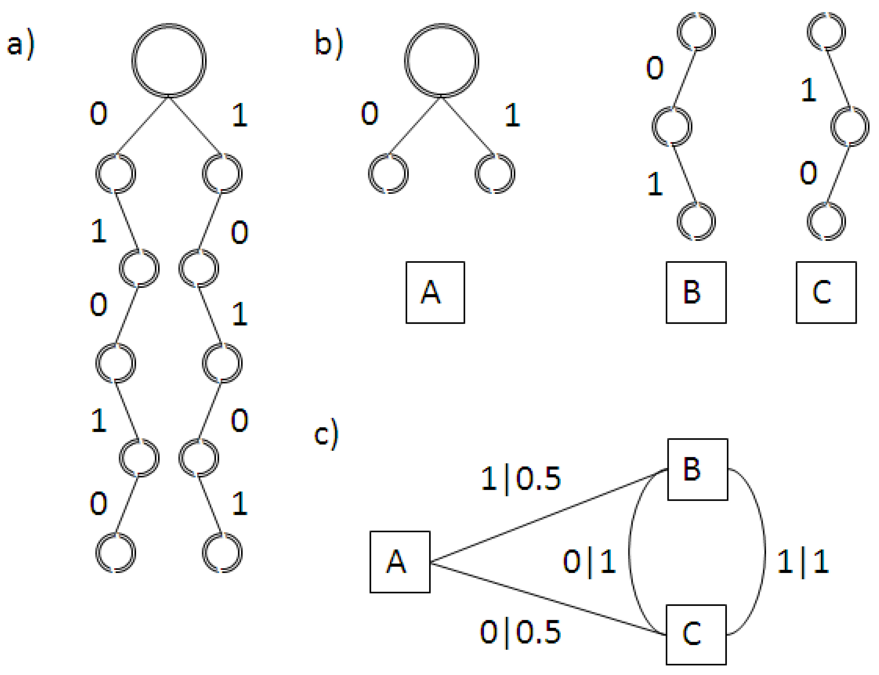
While statistical complexity has the merit of being computable, and in the limited numbers of examples it has been applied to so far, aligns with prevalent conceptual notions of complexity and information distribution, the procedure is practically very unwieldy. The parsing algorithm is computationally expensive and only guarantees pattern recognition up to a chosen length L. Furthermore, any parameterization of the construction of the morphs introduces further estimates (e.g., [35,36]). In order to allow comparability of different systems, one is further required to find the minimum number of morphs and thus the minimal ϵ-machine representation. These difficulties might be the reason that , despite its emphasis on features traditionally highlighted by complexity research, has not become widely used beyond the confines of Crutchfield’s own research group.
C.2. Simplified Statistical Complexity Measures
A number of simplified statistical complexity measures were developed in the wake of Crutchfield and Young [35]. These measures also aim to assign vanishing values to both completely ordered and random distributions. [58] developed a statistical complexity measure that fulfils these requirements by combining the traditional Shannon entropy in Equation (7) with a disequilibrium term . For a set of N outcomes with probabilities they then define statistical complexity as
where
represents the deviation from the uniform distribution. Due to the fact that will vanish for ordered distributions and the disequilibrium term will tend to zero for random distributions, the measure by definition vanishes for both of these cases, although a much cruder estimate than , clearly has the advantage of simplicity. Several variations of Equation (9) have been devised, usually based on a redefinition of the equilibrium value [57,59,73].
The statistical complexity values shown in Section 4.3 were computed according to Equation (9).
D. Phase Space Partitions
Due to the fact the five systems have been chosen such that they can all be represented in the same abstract phase space, one can use the same partition for all of the quantitative measure calculation. Gottwald and Oliver [13] computed one second concept of Boltzmannian entropy for the Kac ring model. They assume the ring’s phase space to consist of particles’ colour states , which can be either white or black. A natural partition for this space is to assume two cells only, one containing all black particles and one containing all white particles. The Shannon entropy can be defined in analogy to this by computing the probabilities for a particle to be found in the black or white box, respectively, as:
Using Equation (7) one then obtains:
One can compute the (simplified) statistical complexity for the rings by inserting Equations (11)–(13) into Equation (9):
The partition used by Gottwald and Oliver [13] does not include any spatial cells. This can be justified by the symmetry of the problems studied and is particularly appropriate for the Kac ring studied by these authors, where we are expecting a disordered state. However, it also means that situations that are clearly ordered and should have low entropy (e.g., a ring where all the black balls are in one half and all the white balls are in the other) are not distinguished from real disordered solutions. In the example above, if only the state of the balls is considered for the phase space partition, both the ring with the clearly distinguishable halves as well as a ring with equal numbers of black and white balls perfectly intermixed have the same entropy and complexity according to Equations (13) and (14), respectively. In this study, expecting the complex ring models to be potential distinguished by just such spatial structures, I have also considered some simple spatial partitions.
For the sake of simplicity I will only divide the ring into fixed and equal segments, each of which accommodates an integer number of balls. Dividing a ring of N balls into m segments, each then containing N/m balls, means that there are now partition cells in total. The probability of finding a ball of a certain colour in the i-th spatial cell is given by:
where and are the number of black and white balls in the i-th cell. Using Equation (7), the Shannon entropy for this partition is given by:
Similarly, the statistical complexity under a spatial partition of m segments can be computed from Equation (9):
In Section 4.3 I show calculations using the traditional partition according to Equations (13) and (14) (Figure 5a and Figure 6a, respectively) and one with ten spatial cells according to Equations (17) and (18) (Figure 5b and Figure 6b, respectively).
E. Random Runs
In addition to the runs discussed in the main part of the paper, I have also conducted simulations in which the models were started off from an uniformly random initial state. The same initial state was chosen for all models. The space-time diagrams of these models are shown in Figure E1.
Comparing Figure E1 to Figure 1, it is immediately apparent that the phenomenologies become more similar to each other. This is especially true with respect to the regular CA90, where no overall nested pattern develops under random initial conditions. Consequently, all five models have almost identical statistical complexity (Figure E2) and entropy (Figure E3) time developments. This further supports my hypothesis that these quantitative measures are not successful in distinguishing complexity from randomness and chaos.
Figure E1.
Space time diagrams of the five models with random initial conditions.
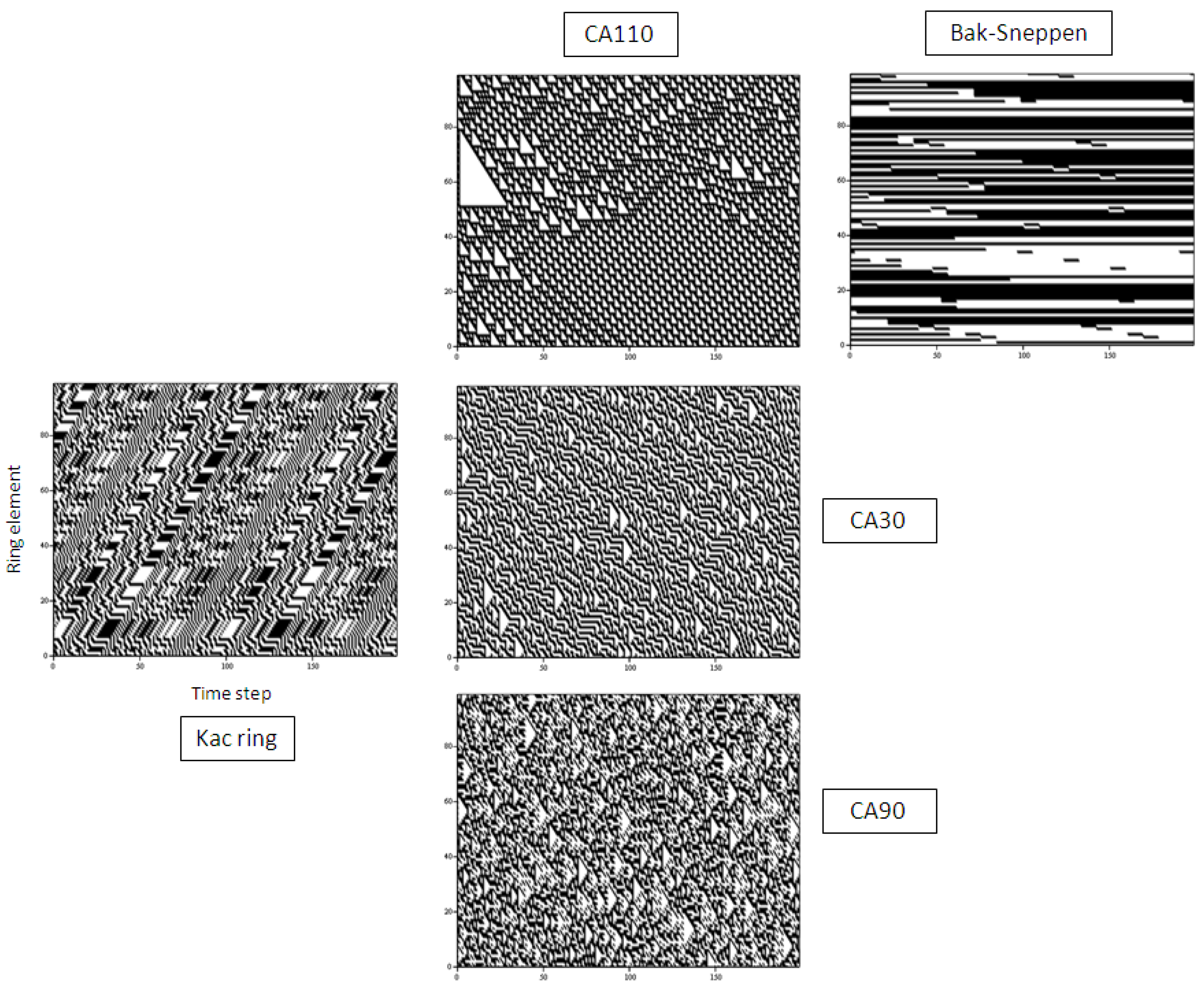
Figure E2.
Statistical complexity of the five models with random initial states. Black: Kac ring. Green: CA30. Blue: CA90. Red: CA110. Yellow: Bak-Sneppen model. In (a) the entropy for no spatial partitions of the ring is shown while in (b) the partition included 10 spatial segments (see Appendix D for details).


Figure E3.
Shannon entropy of the five models with random initial states. Black: Kac ring. Green: CA30. Blue: CA90. Red: CA110. Yellow: Bak-Sneppen model. In (a) the entropy for no spatial partitions of the ring is shown while in (b) the partition included 10 spatial segments (see Appendix D for details).

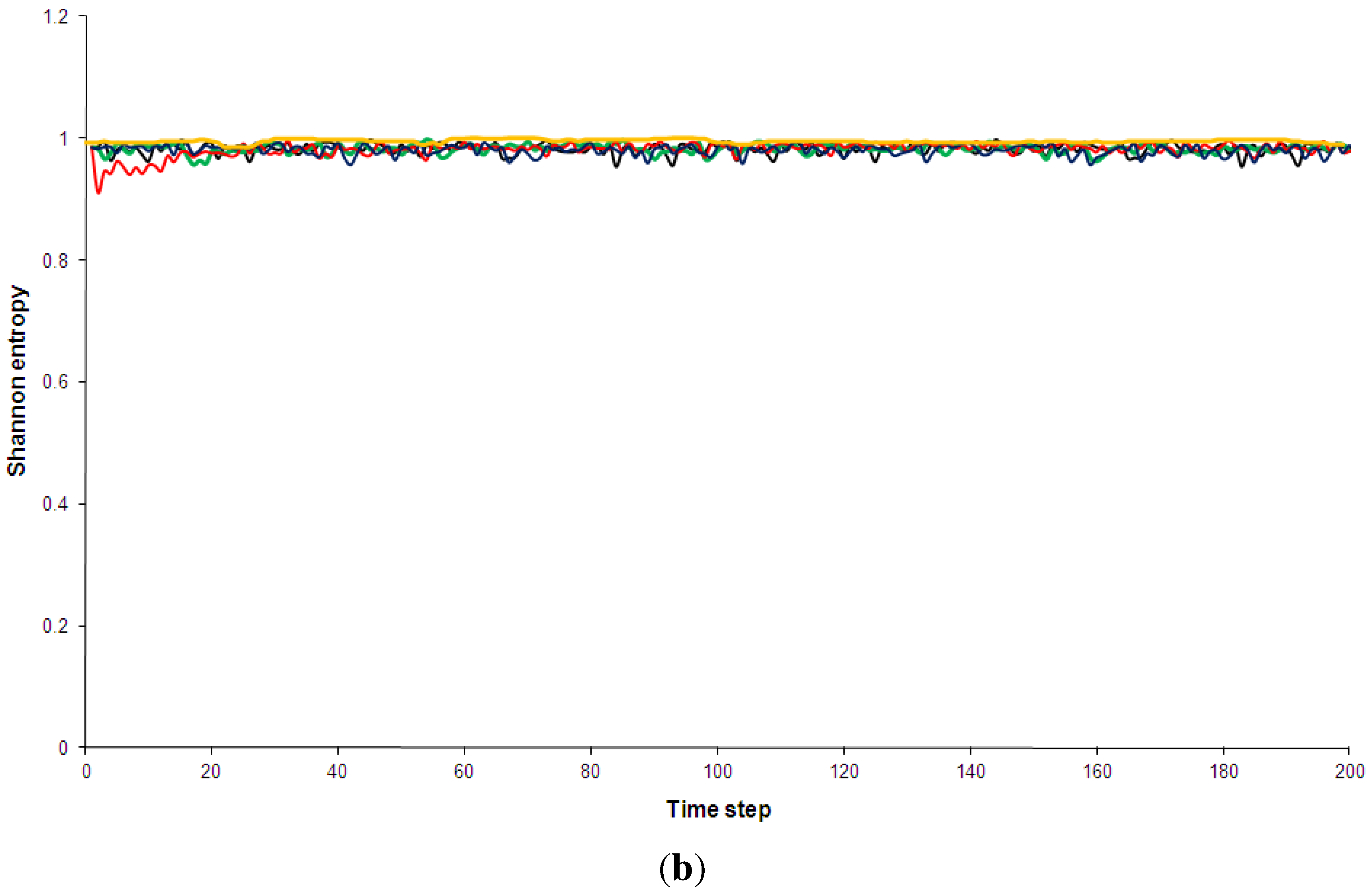
© 2012 by the author; licensee MDPI, Basel, Switzerland. This article is an open access article distributed under the terms and conditions of the Creative Commons Attribution license (http://creativecommons.org/licenses/by/3.0/.)
Share and Cite
MDPI and ACS Style
Zuchowski, L.C. Disentangling Complexity from Randomness and Chaos. Entropy 2012, 14, 177-212. https://doi.org/10.3390/e14020177
AMA Style
Zuchowski LC. Disentangling Complexity from Randomness and Chaos. Entropy. 2012; 14(2):177-212. https://doi.org/10.3390/e14020177
Chicago/Turabian StyleZuchowski, Lena C. 2012. "Disentangling Complexity from Randomness and Chaos" Entropy 14, no. 2: 177-212. https://doi.org/10.3390/e14020177