Temporal Asymmetry, Entropic Irreversibility, and Finite-Time Thermodynamics: From Parmenides–Einstein Time-Reversal Symmetry to the Heraclitan Entropic Arrow of Time

Abstract

In this paper, we combine the two universalisms of thermodynamics and dynamical systems theory to develop a dynamical system formalism for classical thermodynamics. Specifically, using a compartmental dynamical system energy flow model we develop a state-space dynamical system model that captures the key aspects of thermodynamics, including its fundamental laws. In addition, we establish the existence of a unique, continuously differentiable global entropy function for our dynamical system model, and using Lyapunov stability theory we show that the proposed thermodynamic model has finite-time convergent trajectories to Lyapunov stable equilibria determined by the system initial energies. Finally, using the system entropy, we establish the absence of Poincaré recurrence for our thermodynamic model and develop clear and rigorous connections between irreversibility, the second law of thermodynamics, and the entropic arrow of time.

1. Introduction

The arrow of time and the second law of thermodynamics is one of the most famous and controversial problems in physics. The controversy between the course of time (i.e., a timeless universe) and the arrow of time (i.e., a constantly changing universe) can be traced back to the famous dialogues between the ancient Greek philosophers Parmenides and Herakleitos on being and becoming. Parmenides, like Einstein, insisted that time is an illusion, that there is nothing new, and that everything is (being) and will forever be. This statement is, of course, paradoxical since the status quo changed after Parmenides wrote his famous poem. Herakleitos’ aphorism on the other hand is predicated on change (becoming); namely, the universe is in a constant state of flux and nothing is stationary—T$\mathsf{\alpha }\mathsf{\pi }\mathsf{ά}\mathsf{\nu }\mathsf{\tau }\mathsf{\alpha }\mathsf{\rho }\mathsf{\epsilon }\mathsf{ί}\mathsf{\varkappa }\mathsf{\alpha }\mathsf{ί}\mathsf{o}\mathsf{ύ}\mathsf{\delta }\mathsf{έ}\mathsf{\nu }\mathsf{\mu }\mathsf{έ}\mathsf{\nu }\mathsf{\epsilon }\mathsf{\iota }$. Furthermore, Herakleitos goes on to state that the universe evolves in accordance with its own laws which are the only unchangeable things in the universe (i.e., universal conservation and nonconservation laws). His statements that everything is in a state of flux—T$\mathsf{\alpha }\mathsf{\pi }\mathsf{ά}\mathsf{\nu }\mathsf{\tau }\mathsf{\alpha }\mathsf{\rho }\mathsf{\epsilon }\mathsf{ί}$—and that man cannot step into the same river twice, because neither the man nor the river is the same—$\mathsf{\Pi }\mathsf{o}\mathsf{\tau }\mathsf{\alpha }\mathsf{\mu }\mathsf{\epsilon }\mathsf{ί}\mathsf{\varsigma }\mathsf{\tau }\mathsf{o}\mathsf{ί}\mathsf{\varsigma }\mathsf{\alpha }\mathsf{\upsilon }\mathsf{\tau }\mathsf{o}\mathsf{ί}\mathsf{\varsigma }\mathsf{\epsilon }\mathsf{\mu }\mathsf{\beta }\mathsf{\alpha }\mathsf{ί}\mathsf{\nu }\mathsf{o}\mathsf{\mu }\mathsf{\epsilon }\mathsf{\nu }\mathsf{\tau }\mathsf{\epsilon }\mathsf{\varkappa }\mathsf{\alpha }\mathsf{ί}\mathsf{o}\mathsf{\upsilon }\mathsf{\varkappa }\mathsf{\epsilon }\mathsf{\mu }\mathsf{\beta }\mathsf{\alpha }\mathsf{ί}\mathsf{\nu }\mathsf{o}\mathsf{\mu }\mathsf{\epsilon }\mathsf{\nu },\mathsf{\epsilon }\mathsf{ί}\mathsf{\mu }\mathsf{\epsilon }\mathsf{\nu }\mathsf{\tau }\mathsf{\epsilon }\mathsf{\varkappa }\mathsf{\alpha }\mathsf{ί}\mathsf{o}\mathsf{\upsilon }\mathsf{\varkappa }\mathsf{\epsilon }\mathsf{ί}\mathsf{\mu }\mathsf{\epsilon }\mathsf{\nu }$—give the earliest perception of irreversibility of nature and the universe along with time’s arrow. The idea that the universe is in constant change and there is an underlying order to this change—the Logos ($\mathsf{\Lambda }\mathsf{ό}\mathsf{\Upsilon }\mathsf{o}\mathsf{\varsigma }$)—postulates the existence of entropy as a physical property of matter permeating the whole of nature and the universe.

Herakleitos’ statements are completely consistent with the laws of thermodynamics which are intimately connected to the irreversibility of dynamical processes in nature. In addition, his aphorisms go beyond the worldview of thermodynamics and have deep relativistic ramifications to the space-time fabric of the cosmos. Specifically, Herakleitos’ profound statement—All matter is exchanged for energy, and energy for all matter ($\mathsf{\Pi }\mathsf{\upsilon }\mathsf{\rho }\mathsf{ό}\mathsf{\varsigma }\mathsf{\tau }\mathsf{\epsilon }\mathsf{ἀ}\mathsf{\nu }\mathsf{\tau }\mathsf{\alpha }\mathsf{\mu }\mathsf{o}\mathsf{\iota }\mathsf{\beta }\mathsf{ὴ}\mathsf{\tau }\mathsf{ὰ}\mathsf{\pi }\mathsf{ά}\mathsf{\nu }\mathsf{\tau }\mathsf{\alpha }\mathsf{\varkappa }\mathsf{\alpha }\mathsf{ὶ}\mathsf{\pi }\stackrel{\mathsf{͂}}{\mathsf{\upsilon }}\mathsf{\rho }\mathsf{ἁ}\mathsf{\pi }\mathsf{ά}\mathsf{ΰ}\mathsf{\tau }\mathsf{\omega }\mathsf{\nu }$)—is a statement of the law of conservation of mass-energy and is a precursor to the principle of relativity. In describing the nature of the universe Herakleitos postulates that nothing can be created out of nothing, and nothing that disappears ceases to exist. This totality of forms, or mass-energy equivalence, is eternal and unchangeable in a constantly changing universe.

Energy is a concept that underlies our understanding of all physical phenomena and is a measure of the ability of a dynamical system to produce changes (motion) in its own system state as well as changes in the system states of its surroundings. Thermodynamics is a physical branch of science that deals with laws governing energy flow from one body to another and energy transformations from one form to another. These energy flow laws are captured by the fundamental principles known as the first and second laws of thermodynamics. The first law of thermodynamics gives a precise formulation of the equivalence between heat and work and states that among all system transformations, the net system energy is conserved. Hence, energy cannot be created out of nothing and cannot be destroyed; it can merely be transformed from one form to another.

The law of conservation of energy is not a mathematical truth, but rather the consequence of an immeasurable culmination of observations over the chronicle of our civilization, and is a fundamental axiom of the science of heat. The first law does not tell us whether any particular process can actually occur, that is, it does not restrict the ability to convert work into heat or heat into work, except that energy must be conserved in the process. The second law of thermodynamics asserts that, while the system energy is always conserved, it will be degraded to a point where it cannot produce any useful work. Hence, it is impossible to extract work from heat without at the same time discarding some heat, giving rise to an increasing quantity known as entropy.

As discussed in the recent monograph [1], there have been many different presentations of classical thermodynamics with varying hypotheses and conclusions. To exacerbate matters, the careless and considerable differences in the definitions of two of the key notions of thermodynamics—namely, the notions of reversibility and irreversibility—have contributed to the widespread confusion and lack of clarity in the exposition of classical thermodynamics over the past one and a half centuries. For example, the concept of a reversible process as defined by Clausius, Kelvin, Planck, and Carathéodory has very different meanings. In particular, Clausius defines a reversible (umkehrbar) process as a slowly varying process wherein successive states of this process differ by infinitesimals from the equilibrium system states. Such system transformations are commonly referred to as quasistatic transformations in the thermodynamic literature.

Alternatively, Kelvin’s notions of reversibility involve the ability of a system to completely recover its initial state from the final system state. Planck introduced several notions of reversibility. His main notion of reversibility is one of complete reversibility and involves recoverability of the original state of the dynamical system while at the same time restoring the environment to its original condition. Unlike Clausius’ notion of reversibility, Kelvin’s and Planck’s notions of reversibility do not require the system to exactly retrace its original trajectory in reverse order. Carathéodory’s notion of reversibility involves recoverability of the system state in an adiabatic process [2,3,4], resulting in yet another definition of thermodynamic reversibility. These subtle distinctions of (ir)reversibility are often unrecognized in the thermodynamic literature. Notable exceptions to this fact include [1,5,6], with [1,6] providing an excellent exposition of the relation between irreversibility, the second law of thermodynamics, and the arrow of time.

The arrow of time [7] remains one of physics’ most perplexing enigmas [8,9,10,11,12,13]. Even though time is one of the most familiar concepts humankind has ever encountered, it is the least understood. Puzzling questions of time’s mysteries have remained unanswered throughout the centuries—questions such as, Where does time come from? What would our universe look like without time? Can there be more than one dimension to time? Is time truly a fundamental appurtenance woven into the fabric of the universe, or is it just a useful edifice for organizing our perception of events? Why is the concept of time hardly ever found in the most fundamental physical laws of nature and the universe? Can we go back in time? And if so, can we change past events?

Human experience perceives time flow as unidirectional; the present is forever flowing toward the future and away from a forever fixed past. Many scientists have attributed this emergence of the direction of time flow to the second law of thermodynamics due to its intimate connection to the irreversibility of dynamical processes [14]. In this regard, thermodynamics is disjoint from Newtonian and Hamiltonian mechanics (including Einstein’s relativistic and Schrödinger’s quantum extensions), since these theories are invariant under time reversal, that is, they make no distinction between one direction of time and the other. Such theories possess a time-reversal symmetry, wherein, from any given moment of time, the governing laws treat past and future in exactly the same way [15]. For example, a film run backward of a harmonic oscillator over a full period or a planet orbiting the Sun would represent possible events. In contrast, a film run backward of water in a glass coalescing into a solid ice cube or ashes self-assembling into a log of wood would immediately be identified as an impossible event. Over the centuries, many philosophers and scientists shared the views of a Parmenidean frozen river time theory. However, since the advent of the science of thermodynamics in the 19^th century, philosophy and science took a different point of view with the writings of Hegel, Bergson, Heidegger, Clausius, Kelvin, and Boltzmann; one involving time as our existential dimension. The idea that the second law of thermodynamics provides a physical foundation for the arrow of time has been postulated by many authors [9,16,17]. However, a convincing argument of this claim has never been given [1,6,10,12,18].

In this paper, we use energy flow compartmental dynamical system theory to place thermodynamics on a system-theoretic foundation so as to harmonize it with classical mechanics. In particular, we develop a novel formulation of thermodynamics that can be viewed as a moderate-sized system theory as compared to statistical thermodynamics. This middle-ground theory involves deterministic large-scale dynamical system models that bridge the gap between classical and statistical thermodynamics. Specifically, since thermodynamic models are concerned with energy flow among subsystems, we use a state space formulation to develop a nonlinear compartmental dynamical system model that is characterized by energy conservation laws capturing the exchange of energy between coupled macroscopic subsystems. Furthermore, using graph-theoretic notions, we state two thermodynamic axioms consistent with the zeroth and second laws of thermodynamics, which ensure that our large-scale dynamical system model gives rise to a thermodynamically consistent energy flow model. Specifically, using a large-scale dynamical systems theory perspective for thermodynamics, we show that our compartmental dynamical system model leads to a precise formulation of the equivalence between work energy and heat in a large-scale dynamical system.

Next, we give a deterministic definition of entropy for a large-scale dynamical system that is consistent with the classical thermodynamic definition of entropy, and we show that it satisfies a Clausius-type inequality leading to the law of entropy nonconservation. However, unlike classical thermodynamics, wherein entropy is not defined for arbitrary states out of equilibrium, our definition of entropy holds for nonequilibrium dynamical systems. Then, using Lyapunov stability theory, we show that in the absence of energy exchange with the environment our thermodynamically consistent large-scale nonlinear dynamical system model possesses a continuum of equilibria and is semistable, that is, it has subsystem energies convergent to Lyapunov stable energy equilibria determined by the large-scale system’s initial subsystem energies.

For our thermodynamically consistent dynamical system model, we further establish the existence of a unique continuously differentiable global entropy function for all equilibrium and nonequilibrium states. Using this global entropy function, we go on to establish a clear connection between thermodynamics and the arrow of time. Specifically, we rigorously show the state irrecoverability and hence the state irreversibility [6,19] nature of thermodynamics. In particular, we show that for every nonequilibrium system state and corresponding system trajectory of our thermodynamically consistent large-scale nonlinear dynamical system, there does not exist a state such that the corresponding system trajectory completely recovers the initial system state of the dynamical system and at the same time restores the energy supplied by the environment back to its original condition. This, along with the existence of a global strictly increasing entropy function on every nontrivial system trajectory, gives a clear time-reversal asymmetry characterization of thermodynamics, establishing the emergence of the direction of time flow. Finally, since for every physical system energy and temperature equipartition is achieved in finite time rather than merely asymptotically, we merge the theories of semistability and finite-time stability developed in [20,21,22] to develop a mathematically rigorous framework for finite-time thermodynamics.

2. Dynamical System Model

In this section, we establish notation and provide a general axiomatic definition of a dynamical system. The notation used in this paper is fairly standard. Specifically, $\mathbb{R}$ denotes the set of real numbers, ${\overline{\mathbb{Z}}}_{+}$ (respectively, ${\mathbb{Z}}_{+}$) denotes the set of nonnegative (respectively, positive) integers, ${\mathbb{R}}^q$ denotes the set of $q\times 1$ column vectors, ${(·)}^{\text{T}}$ denotes transpose, and $I_q$ or I denotes the $q\times q$ identity matrix. For $z\in {\mathbb{R}}^q$ we write $z\ge \ge 0$ (respectively, $z>>0$) to indicate that every component of z is nonnegative (respectively, positive). In this case we say that z is nonnegative or positive, respectively. Furthermore, let ${\overline{\mathbb{R}}}_{+}^q$ and ${\mathbb{R}}_{+}^q$ denote the nonnegative and positive orthants of ${\mathbb{R}}^q$, that is, if $z\in {\mathbb{R}}^q$, then $z\in {\overline{\mathbb{R}}}_{+}^q$ and $z\in {\mathbb{R}}_{+}^q$ are equivalent, respectively, to $z\ge \ge 0$ and $z>>0$. Finally, let $\partial \mathcal{S}$, $\mathring{\mathcal{S}}$, and $\overline{\mathcal{S}}$ denote the boundary, the interior, and the closure of the set $\mathcal{S}$, respectively.

We write ‖ · ‖ for the Euclidean vector norm, $V^{\prime }\left(z\right)$ for the Fréchet derivative of V at z, ${\mathcal{B}}_{\epsilon }\left(\alpha \right)$, $\alpha \in {\mathbb{R}}^q$, $\epsilon >0$, for the open ball centered at α with radius ε, and $z\left(t\right)\to \mathcal{M}$ as $t\to \infty$ to denote that $z\left(t\right)$ approaches the set $\mathcal{M}$ (that is, for each $\epsilon >0$ there exists $T>0$ such that dist$\left(z\right(t),\mathcal{M})<\epsilon$ for all $t>T$, where dist$(p,\mathcal{M})\triangleq {inf}_{z\in \mathcal{M}}\parallel p-z\parallel$). Finally, the notions of openness, convergence, continuity, and compactness that we use throughout the paper refer to the topology generated on $\mathcal{D}\subseteq {\mathbb{R}}^q$ by the norm $\parallel ·\parallel$.

Next, we define a dynamical system as a precise mathematical object satisfying a set of axioms. For this definition, let $\mathcal{U}$ denote an input space that consists of bounded continuous U-valued functions on $[0,\infty )$. The set $U\subseteq {\mathbb{R}}^m$ contains the set of input values, that is, at any time $t\ge t_0$, $u\left(t\right)\in U$. The space $\mathcal{U}$ is assumed to be closed under the shift operator, that is, if $u\in \mathcal{U}$, then the function $u_T$ defined by $u_T\left(t\right)\triangleq u(t+T)$ is contained in $\mathcal{U}$ for all $T\ge 0$. Furthermore, we let $\mathcal{Y}$ denote an output space that consists of continuous Y-valued functions on $[0,\infty )$. The set $Y\subseteq {\mathbb{R}}^l$ contains the set of output values, that is, each value of $y\left(t\right)\in Y$, $t\ge t_0$. The space $\mathcal{Y}$ is assumed to be closed under the shift operator, that is, if $y\in \mathcal{Y}$, then the function $y_T$ defined by $y_T\left(t\right)\triangleq y(t+T)$ is contained in $\mathcal{Y}$ for all $T\ge 0$.

Definition 2.1 

Let $\mathcal{D}$ be a Euclidean space with norm ∥ · ∥. A dynamical system on $\mathcal{D}$ is the octuple $(\mathcal{D},\mathcal{U},U,\mathcal{Y},Y,$$[0,\infty ),s,h)$, where $s:[0,\infty )\times \mathcal{D}\times \mathcal{U}\to \mathcal{D}$ and $h:\mathcal{D}\times U\to Y$ are such that the following axioms hold:

(i)

(Continuity): $s(·,·,u)$ is jointly continuous for all $u\in \mathcal{U}$.

(ii)

(Consistency): $s(t_0,x_0,u)=x_0$ for all $t_0\in \mathbb{R}$, $x_0\in \mathcal{D}$, and $u\in \mathcal{U}$.

(iii)

(Determinism): $s(t,x_0,u_1)=s(t,x_0,u_2)$ for all $t\in [t_0,\infty )$, $x_0\in \mathcal{D}$, and $u_1$, $u_2\in \mathcal{U}$ satisfying $u_1\left(\tau \right)=u_2\left(\tau \right)$, $\tau \le t$.

(iv)

(Semigroup property): $s(\tau ,s(t,x_0,u),u)=s(t+\tau ,x_0,u)$ for all $x_0\in \mathcal{D}$, $u\in \mathcal{U}$, and τ, $t\in [t_0,\infty )$.

(v)

(Read-out map): For every $x_0\in \mathcal{D}$, $u\in \mathcal{U}$, and $t_0\in \mathbb{R}$, there exists $y\in \mathcal{Y}$ such that$y\left(t\right)=h\left(s\right(t,x_0,$$u),u(t\left)\right)$ for all $t\ge t_0$.

We denote the dynamical system $(\mathcal{D},\mathcal{U},U,\mathcal{Y},Y,$ $[0,\infty ),s,h)$ by $\mathcal{G}$. Furthermore, we refer to the map $s(·,·,·)$ as the flow or trajectory of $\mathcal{G}$ corresponding to $x_0\in \mathcal{D}$, and for a given $s(t,x_0,u)$, $t\ge t_0$, $u\in \mathcal{U}$, we refer to $x_0\in \mathcal{D}$ as an initial condition of $\mathcal{G}$. Given $t\in \mathbb{R}$, we denote the map $s(t,·,·):\mathcal{D}\times \mathcal{U}\to \mathcal{D}$ by $s_t(x_0,u)$. Hence, for a fixed $t\in \mathbb{R}$ the set of mappings defined by $s_t(x_0,u)=s(t,x_0,u)$ for every $x_0\in \mathcal{D}$ and $u\in \mathcal{U}$ gives the flow of $\mathcal{G}$. In particular, if ${\mathcal{D}}_0$ is a collection of initial conditions such that ${\mathcal{D}}_0\subset \mathcal{D}$, then the flow $s_t:{\mathcal{D}}_0\times \mathcal{U}\to \mathcal{D}$ is the motion of all points $x_0\in {\mathcal{D}}_0$ or, equivalently, the image of ${\mathcal{D}}_0\subset \mathcal{D}$ under the flow $s_t$, that is, $s_t({\mathcal{D}}_0,\mathcal{U})\subset \mathcal{D}$, where $s_t({\mathcal{D}}_0,\mathcal{U})\triangleq \{y:y=s_t(x_0,u)\mathrm{for}\mathrm{all}{x}_0\in \mathcal{D}$ and $u\in \mathcal{U}\}$. Alternatively, if the initial condition $x_0\in \mathcal{D}$ is fixed and we let $[t_0,t_1]\subset \mathbb{R}$ and $u\in \mathcal{U}$, then the mapping $s(·,x_0,u):[t_0,t_1]\to \mathcal{D}$ defines the solution curve or trajectory of the dynamical system $\mathcal{G}$. Hence, the mapping $s(·,x_0,u)$ generates a graph in $[t_0,t_1]\times \mathcal{D}$ identifying the trajectory corresponding to the motion along a curve through the point $x_0$ with input $u\in \mathcal{U}$ in a subset $\mathcal{D}$ of the state space. Given $x\in \mathcal{D}$ and $u\in \mathcal{U}$, we denote the map $s(·,x,u):\mathbb{R}\to \mathcal{D}$ by $s^x(t,u)$.

In general, the output of $\mathcal{G}$ depends on both the present input of $\mathcal{G}$ and the past history of $\mathcal{G}$. Hence, the output at some time $t_1$ depends on the state $s(t_1,x_0,u)$ of $\mathcal{G}$, which effectively serves as an information storage (memory) of past history. Furthermore, the determinism axiom ensures that the state and thus the output before some time $t_1$ are not influenced by the values of the output after time $t_1$. Hence, future inputs to $\mathcal{G}$ do not affect past and present outputs of $\mathcal{G}$. This is simply a statement of causality that holds for all physical systems. Finally, we note that the read-out map is memoryless in the sense that outputs only depend on the instantaneous (present) values of the state and input.

The dynamical system $\mathcal{G}$ is isolated if $u\left(t\right)\equiv 0$. Furthermore, an equilibrium point of the isolated dynamical system $\mathcal{G}$ is a point $x_{\mathrm{e}}\in \mathcal{D}$ satisfying $s(t,x_{\mathrm{e}},0)=x_{\mathrm{e}},t\ge t_0$. An equilibrium point $x_{\mathrm{e}}\in {\mathcal{D}}_{\mathrm{c}}\subseteq \mathcal{D}$ of the isolated dynamical system $\mathcal{G}$ is Lyapunov stable with respect to the positively invariant set ${\mathcal{D}}_{\mathrm{c}}$ if, for every relatively open subset ${\mathcal{N}}_{\epsilon }$ of ${\mathcal{D}}_{\mathrm{c}}$ containing $x_{\mathrm{e}}$, there exists a relatively open subset ${\mathcal{N}}_{\delta }$ of ${\mathcal{D}}_{\mathrm{c}}$ containing $x_{\mathrm{e}}$ such that $s_t({\mathcal{N}}_{\delta },\mathcal{U})\subset {\mathcal{N}}_{\epsilon }$ for all $t\ge t_0$, where $\mathcal{U}=\{u:\mathbb{R}\to {\mathbb{R}}^m:u\left(t\right)\equiv 0\}$. An equilibrium point $x_{\mathrm{e}}\in {\mathcal{D}}_{\mathrm{c}}$ of the isolated dynamical system $\mathcal{G}$ is called semistable if it is Lyapunov stable and there exists a relatively open subset $\mathcal{N}$ of ${\mathcal{D}}_{\mathrm{c}}$ containing $x_{\mathrm{e}}$ such that for all initial conditions in $\mathcal{N}$, the trajectory of $\mathcal{G}$ converges to a Lyapunov stable equilibrium point, that is, $\parallel s(t,x,0)-y\parallel \to 0$ as $t\to \infty$, where $y\in {\mathcal{D}}_{\mathrm{c}}$ is a Lyapunov stable equilibrium point of $\mathcal{G}$ and $x\in \mathcal{N}$. The isolated dynamical system $\mathcal{G}$ is said to be semistable if every equilibrium point of $\mathcal{G}$ is semistable.

Finally, for a given interval $[t_0,t_1]$, where $0\le t_0<t_1<\infty$, let ${\mathcal{W}}_{[t_0,t_1]}$ denote the set of all possible trajectories of given by

$$\begin{array}{c}\hfill \begin{array}{cc}\hfill {\mathcal{W}}_{[t_0,t_1]}& \{s^x:[t_0,t_1]\times \mathcal{U}\to \mathcal{D}:s^x(·,u(·))\text{satisfies Axioms }\left(\mathrm{i}\right)–\left(\mathrm{iv}\right)\hfill \\ & \text{of Definition 2.1},x\in \mathcal{D},\text{and }u(·)\in \mathcal{U}\}\hfill \end{array}\end{array}$$

(1)

where $s^x(·,u(·))$ denotes the solution curve or trajectory of $\mathcal{G}$ for a given fixed initial condition $x\in \mathcal{D}$ and input $u(·)\in \mathcal{U}$.

3. Reversibility, Irreversibility, Recoverability and Irrecoverability

The notions of reversibility, irreversibility, recoverability, and irrecoverability all play a central role in thermodynamic processes. In this section, we define the notions of R-state reversibility, state reversibility, and state recoverability of a dynamical system $\mathcal{G}$. R-state reversibility concerns the existence of a system state with the property that a transformed system trajectory through an involution operator R is an image of a given system trajectory of $\mathcal{G}$ on a specified finite time interval. State reversibility concerns the existence of a system state with the property that the resulting system trajectory is the time-reversed image of a given system trajectory of $\mathcal{G}$ on a specified finite time interval. Finally, state recoverability concerns the existence of a system state with the property that the resulting system trajectory completely recovers the initial state of the dynamical system over a finite time interval.

For the results of this section we use the definition of a dynamical system given in Definition 2.1. We start by establishing the notions of (ir)reversibility and (ir)recoverability of a dynamical system $\mathcal{G}$ defined on a Euclidean space $\mathcal{D}$.

Definition 3.1 

Consider the dynamical system $\mathcal{G}$ defined on $\mathcal{D}$. Let $R:\mathcal{D}\to \mathcal{D}$ be an involutive operator (that is, $R^2=I_{\mathcal{D}}$, where $I_{\mathcal{D}}$ denotes the identity operator on $\mathcal{D}$) and let $s^x(·,u(·))\in {\mathcal{W}}_{[t_0,t_1]}$, where $u(·)\in \mathcal{U}$. The function $s^{-x}:[t_0,t_1]\times \mathcal{U}\to \mathcal{D}$ is an R-reversed trajectory of $s^x(·,u(·))$ if there exist an input $u^{-}(·)\in \mathcal{U}$ and a continuous, strictly increasing function $\tau :[t_0,t_1]\to [t_0,t_1]$ such that $\tau \left(t_0\right)=t_0$, $\tau \left(t_1\right)=t_1$, and

$$\begin{array}{c}\hfill s^{-x}(t,u^{-}\left(t\right))=R{s}^x(t_0+t_1-\tau \left(t\right),u(t_0+t_1-\tau \left(t\right))),t\in [t_0,t_1]\end{array}$$

(2)

Definition 3.2 

Consider the dynamical system $\mathcal{G}$ defined on $\mathcal{D}$. Let $R:\mathcal{D}\to \mathcal{D}$ be an involutive operator, let $r:\mathcal{U}\times \mathcal{Y}\to \mathbb{R}$, and let $s^x(·,u(·))\in {\mathcal{W}}_{[t_0,t_1]}$, where $u(·)\in \mathcal{U}$. $s^x(·,u(·))$ is an R-reversible trajectory of $\mathcal{G}$ if there exists an input $u^{-}(·)\in \mathcal{U}$ such that $s^{-x}(·,u^{-}(·))\in {\mathcal{W}}_{[t_0,t_1]}$ and

$$\begin{array}{c}\hfill {\int }_{t_0}^{t_1}r(u\left(t\right),y\left(t\right))\mathrm{d}t+{\int }_{t_0}^{t_1}r(u^{-}\left(t\right),y^{-}\left(t\right))\mathrm{d}t=0\end{array}$$

(3)

where $y^{-}(·)$ denotes the read-out map for the R-reversed trajectory of $s^x(·,u(·))$. Furthermore, $\mathcal{G}$ is an R-state reversible dynamical system if for every $x\in \mathcal{D}$, $s^x(·,u(·))$, where $u(·)\in \mathcal{U}$ is an R-reversible trajectory of $\mathcal{G}$.

In classical mechanics, R is a transformation that reverses the sign of all system momenta and magnetic fields, whereas in classical reversible thermodynamics R can be taken to be the identity operator. Note that if $R=I_{\mathcal{D}}$, then $s^x(·,u(·))$, where $u(·)\in \mathcal{U}$ is an $I_{\mathcal{D}}$-reversible trajectory or, simply, $s^x(·,u(·))$ is a reversible trajectory. Furthermore, we say that $\mathcal{G}$ is a state reversible dynamical system if and only if for every $x\in \mathcal{D}$, $s^x(·,u(·))$, where $u(·)\in \mathcal{U}$ is a reversible trajectory of $\mathcal{G}$. Note that unlike state reversible systems, R-state reversible dynamical systems need not retrace every stage of the original system trajectory in reverse order, nor is it necessary for the dynamical system to recover the initial system state.

The function $r(u,y)$ in Definition 3.2 is a generalized power supply from the environment to the dynamical system through the system’s input-output ports $(u,y)$. Hence, Equation (3) ensures that the total generalized energy supplied to the dynamical system $\mathcal{G}$ by the environment is returned to the environment over a given R-reversible trajectory starting and ending at any given (not necessarily the same) state $x\in \mathcal{D}$. Furthermore, Equation (3) ensures that a reversible process completely restores the original dynamic state of a system and at the same time restores the energy supplied by the environment back to its original condition. The following result provides sufficient conditions for the existence of an R-reversible trajectory of a nonlinear dynamical system $\mathcal{G}$, and hence, establishes sufficient conditions for R-state reversibility of the dynamical system $\mathcal{G}$.

Theorem 3.1 

Consider the dynamical system $\mathcal{G}$ defined on $\mathcal{D}$. Let $R:\mathcal{D}\to \mathcal{D}$ be an involutive operator, and let $s^x(·,u(·))\in {\mathcal{W}}_{[t_0,t_1]}$, where $u(·)\in \mathcal{U}$. Assume there exist a continuous function $V:\mathcal{D}\to \mathbb{R}$ and a function $r:\mathcal{U}\times \mathcal{Y}\to \mathbb{R}$ such that $V\left(x\right)=V\left(Rx\right)$, $x\in \mathcal{D}$, and for every $x\in \mathcal{D}$ and all ${\widehat{t}}_0$, ${\widehat{t}}_1$, $t_0\le {\widehat{t}}_0<{\widehat{t}}_1\le t_1$,

$$\begin{array}{c}\hfill V\left(s^x({\widehat{t}}_1,u\left({\widehat{t}}_1\right))\right)\ge V\left(s^x({\widehat{t}}_0,u\left({\widehat{t}}_0\right))\right)+{\int }_{{\widehat{t}}_0}^{{\widehat{t}}_1}r(u\left(t\right),y\left(t\right))\mathrm{d}t\end{array}$$

(4)

Furthermore, assume there exists $\mathcal{M}\subset \mathcal{D}$ such that for all ${\widehat{t}}_0$, ${\widehat{t}}_1$, $t_0\le {\widehat{t}}_0<{\widehat{t}}_1\le t_1$, and $s^x(t,u\left(t\right))\notin \mathcal{M}$, $t\in [{\widehat{t}}_0,{\widehat{t}}_1]$, Equation (4) holds as a strict inequality. If $s^x(·,u(·))$ is an R-reversible trajectory of $\mathcal{G}$, then $s^x(t,u\left(t\right))\in \mathcal{M}$, $t\in [t_0,t_1]$.

Proof. 

Let $s^x(·,u(·))\in {\mathcal{M}}_{[t_0,t_1]}$, where $u(·)\in \mathcal{U}$, be an R-reversible trajectory of $\mathcal{G}$ so that there exists $u^{-}(·)\in \mathcal{U}$ such that $s^{-x}(·,u^{-}(·))\in {\mathcal{M}}_{[t_0,t_1]}$. Suppose, ad absurdum, there exists $t\in [t_0,t_1]$ such that $s^x(t,u\left(t\right))\notin \mathcal{M}$. Now, it follows that there exists an interval $[{\widehat{t}}_0,{\widehat{t}}_1]\subset [t_0,t_1]$ such that for $t_0\le {\widehat{t}}_0<{\widehat{t}}_1\le t_1$,

$$\begin{array}{c}\hfill V\left(s^x({\widehat{t}}_1,u\left({\widehat{t}}_1\right))\right)>V\left(s^x({\widehat{t}}_0,u\left({\widehat{t}}_0\right))\right)+{\int }_{{\widehat{t}}_0}^{{\widehat{t}}_1}r(u\left(t\right),y\left(t\right))\mathrm{d}t\end{array}$$

(5)

which further implies that

$$\begin{array}{c}\hfill V\left(s^x(t_1,u\left(t_1\right))\right)>V\left(s^x(t_0,u\left(t_0\right))\right)+{\int }_{t_0}^{t_1}r(u\left(t\right),y\left(t\right))\mathrm{d}t\end{array}$$

(6)

Next, since $s^{-x}(·,u^{-}(·))\in {\mathcal{M}}_{[t_0,t_1]}$, where $u^{-}(·)\in \mathcal{U}$, it follows that

$$\begin{array}{c}\hfill V\left(s^{-x}(t_1,u^{-}\left(t_1\right))\right)\ge V\left(s^{-x}(t_0,u^{-}\left(t_0\right))\right)+{\int }_{t_0}^{t_1}r(u^{-}\left(t\right),y^{-}\left(t\right))\mathrm{d}t\end{array}$$

(7)

Now, adding Equations (6) and (7), using the definition of $s^{-x}(·,u^{-}(·))$, using the fact that $V\left(x\right)=V\left(Rx\right)$, $x\in \mathcal{D}$, and using Equation (3) yields

$$\begin{array}{c}\hfill V\left(s^x(t_0,u\left(t_0\right))\right)+V\left(s^x(t_1,u\left(t_1\right))\right)>V\left(s^x(t_0,u\left(t_0\right))\right)+V\left(s^x(t_1,u\left(t_1\right))\right)\end{array}$$

which is a contradiction. Hence, $s^x(t,u\left(t\right))\in \mathcal{M}$, $t\in [t_0,t_1]$. ☐

It is important to note that since $V:\mathcal{D}\to \mathbb{R}$ in Theorem 3.1 is not sign definite, Theorem 3.1 also holds for the case where the inequality in Equation (4) is reversed. The following corollary to Theorem 3.1 is immediate.

Corollary 3.1 

Consider the dynamical system $\mathcal{G}$ defined on $\mathcal{D}$. Let $R:\mathcal{D}\to \mathcal{D}$ be an involutive operator, let $\mathcal{M}\subset \mathcal{D}$, and let $s^x(·,u(·))\in {\mathcal{W}}_{[t_0,t_1]}$, where $u(·)\in \mathcal{U}$. Assume there exists a continuous function $V:\mathcal{D}\to \mathbb{R}$ such that $V\left(x\right)=V\left(Rx\right)$, $x\in \mathcal{D}$, and for $s^x(t,u\left(t\right))\notin \mathcal{M}$, $t\in [t_1,t_2]$, $V\left(s(t,x_0,u(·))\right)$ is a strictly increasing (respectively, decreasing) function of time. If $s^x(·,u(·))$ is an R-reversible trajectory of $\mathcal{G}$, then $s^x(t,u\left(t\right))\in \mathcal{M}$, $t\in [t_0,t_1]$.

Proof. 

The proof is a direct consequence of Theorem 3.1 with $r(u,y)\equiv 0$ and the fact that Theorem 3.1 also holds for the case when the inequality in Equation (4) is reversed. ☐

It follows from Corollary 3.1 that if, for a given dynamical system $\mathcal{G}$, there exists an R-reversible trajectory of $\mathcal{G}$, then there does not exist a function of the state of the system that strictly decreases or strictly increases in time on any trajectory of $\mathcal{G}$ lying in $\mathcal{M}$. In this case, the existence of a completely ordered time set having a topological structure involving a closed set homeomorphic to the real line cannot be established. Such systems, which include lossless Newtonian and Hamiltonian systems, are time-reversal symmetric and hence lack an inherent time direction. However, that is not the case with thermodynamic systems.

Next, we present a notion of state recoverability of a dynamical system $\mathcal{G}$.

Definition 3.3 

Consider the dynamical system $\mathcal{G}$ defined on $\mathcal{D}$. Let $r:\mathcal{U}\times \mathcal{Y}\to \mathbb{R}$, and let $s^x(·,u(·))\in {\mathcal{W}}_{[t_0,t_1]}$, where $u(·)\in \mathcal{U}$. $s^x(·,u(·))$ is a recoverable trajectory of $\mathcal{G}$ if there exist $u^{-}(·)\in \mathcal{U}$ and $t_2>t_1$ such that $u^{-}:[t_1,t_2]\to U$,

$$\begin{array}{c}\hfill s(t_2,s^x(t_1,u\left(t_1\right)),u^{-}\left(t_2\right))=s^x(t_0,u\left(t_0\right))\end{array}$$

(8)

and

$$\begin{array}{c}\hfill {\int }_{t_0}^{t_1}r(u\left(t\right),y\left(t\right))\mathrm{d}t+{\int }_{t_1}^{t_2}r(u^{-}\left(t\right),y^{-}\left(t\right))\mathrm{d}t=0\end{array}$$

(9)

where $y^{-}(·)$ denotes the read-out map for the trajectory $s(·,s^x(t_1,u\left(t_1\right)),$$u^{-}(·))$. Furthermore, $\mathcal{G}$ is a state recoverable dynamical system if for every $x\in \mathcal{D}$, $s^x(·,u(·))$ is a recoverable trajectory of $\mathcal{G}$.

It follows from the definition of state recoverability that the way in which the initial dynamical system state is restored may be chosen freely so long as Equation (9) is satisfied. Hence, unlike R-state reversibility, it is not necessary for the dynamical system to recover the initial state of the system through an involutive transformation of the system trajectory. Furthermore, unlike state reversibility, it is not necessary for the dynamical system to retrace every stage of the original trajectory in the reverse order. However, Equation (9) ensures that the recoverable process completely restores the original dynamic state and at the same time restores the energy supplied by the environment back to its original condition. This notion of recoverability is closely related to Planck’s notion of complete reversibility, wherein the initial system state is restored in the totality of nature (“die gesamte Natur"). The following result provides a sufficient condition for the existence of a recoverable trajectory of a nonlinear dynamical system $\mathcal{G}$, and hence, establishes sufficient conditions for state recoverability of $\mathcal{G}$.

Theorem 3.2 

Consider the dynamical system $\mathcal{G}$ defined on $\mathcal{D}$. Let $s^x(·,u(·))\in {\mathcal{W}}_{[t_0,t_1]}$, where $u(·)\in \mathcal{U}$. Assume there exist a continuous function $V:\mathcal{D}\to \mathbb{R}$ and a function $r:\mathcal{U}\times \mathcal{Y}\to \mathbb{R}$ such that for every $x\in \mathcal{D}$ and all ${\widehat{t}}_0$, ${\widehat{t}}_1$, $t_0\le {\widehat{t}}_0<{\widehat{t}}_1\le t_1$,

$$\begin{array}{ccc}\hfill V\left(s^x({\widehat{t}}_1,u\left({\widehat{t}}_1\right))\right)& \ge & V\left(s^x({\widehat{t}}_0,u\left({\widehat{t}}_0\right))\right)+{\int }_{{\widehat{t}}_0}^{{\widehat{t}}_1}r(u\left(t\right),y\left(t\right))\mathrm{d}t\hfill \end{array}$$

(10)

Furthermore, assume there exists $\mathcal{M}\subset \mathcal{D}$ such that for all ${\widehat{t}}_0$, ${\widehat{t}}_1$, $t_0\le {\widehat{t}}_0<{\widehat{t}}_1\le t_1$, and $s^x(t,u\left(t\right))\notin \mathcal{M}$, $t\in [{\widehat{t}}_0,{\widehat{t}}_1]$, Equation (10) holds as a strict inequality. If $s^x(·,u(·))$ is a recoverable trajectory of $\mathcal{G}$, then $s^x(t,u\left(t\right))\in \mathcal{M}$, $t\in [t_0,t_1]$.

Proof. 

Let $s^x(·,u(·))\in {\mathcal{W}}_{[t_0,t_1]}$, where $u(·)\in \mathcal{U}$, be a recoverable trajectory of $\mathcal{G}$ so that there exist $u^{-}(·)\in \mathcal{U}$ and $t_2>t_1$ such that $s(t_2,s^x(t_1,u\left(t_1\right)),u^{-}\left(t_2\right))=s^x(t_0,u\left(t_0\right))$. Suppose, ad absurdum, there exists $t\in [t_0,t_1]$ such that $s^x(t,u\left(t\right))\notin \mathcal{M}$. Now, it follows that there exists an interval $[{\widehat{t}}_0,{\widehat{t}}_1]\subset [t_0,t_1]$ such that for $t_0\le {\widehat{t}}_0<{\widehat{t}}_1\le t_1$,

$$\begin{array}{c}\hfill V\left(s^x({\widehat{t}}_1,u\left({\widehat{t}}_1\right))\right)>V\left(s^x({\widehat{t}}_0,u\left({\widehat{t}}_0\right))\right)+{\int }_{{\widehat{t}}_0}^{{\widehat{t}}_1}r(u\left(t\right),y\left(t\right))\mathrm{d}t\end{array}$$

(11)

which further implies that

$$\begin{array}{c}\hfill V\left(s^x(t_1,u\left(t_1\right))\right)>V\left(s^x(t_0,u\left(t_0\right))\right)+{\int }_{t_0}^{t_1}r(u\left(t\right),y\left(t\right))\mathrm{d}t\end{array}$$

(12)

Next, it follows from Equation (10) with $t_2>t_1$ that

$$\begin{array}{c}\hfill V\left(s(t_2,s^x(t_1,u\left(t_1\right)),u^{-}\left(t_2\right))\right)\ge V\left(s(t_1,s^x(t_1,u\left(t_1\right)),u^{-}\left(t_1\right))\right)+{\int }_{t_1}^{t_2}r(u^{-}\left(t\right),y^{-}\left(t\right))\mathrm{d}t\end{array}$$

(13)

Now, adding Equations (12) and (13), using the definition of $s(t_2,s^x(t_1,u\left(t_1\right),$$u^{-}\left(t_2\right)\left)\right)$, and using Equation (9) yields

$$\begin{array}{c}\hfill V\left(s^x(t_0,u\left(t_0\right))\right)+V\left(s^x(t_1,u\left(t_1\right))\right)>V\left(s^x(t_0,u\left(t_0\right))\right)+V\left(s^x(t_1,u\left(t_1\right))\right)\end{array}$$

which is a contradiction. Hence, $s^x(t,u\left(t\right))\in \mathcal{M}$, $t\in [t_0,t_1]$. ☐

The following corollary to Theorem 3.2 is immediate.

Corollary 3.2 

Consider the dynamical system $\mathcal{G}$ defined on $\mathcal{D}$. Let $\mathcal{M}\subset \mathcal{D}$, and let $s^x(·,u(·))\in {\mathcal{W}}_{[t_0,t_1]}$, where $u(·)\in \mathcal{U}$. Assume there exists a continuous function $V:\mathcal{D}\to \mathbb{R}$ such that for $s^x(t,u\left(t\right))\notin \mathcal{M}$, $t\in [t_0,t_1]$, $V(s(t,x_0,u(·))$ is a strictly increasing (respectively, decreasing) function of time. If $s^x(·,u(·))$ is a recoverable trajectory of $\mathcal{G}$, then $s^x(t,u\left(t\right))\in \mathcal{M}$, $t\in [t_0,t_1]$.

Proof. 

The proof is a direct consequence of Theorem 3.2 with $r(u,y)\equiv 0$ and the fact that Theorem 3.2 also holds for the case when the inequality in Equation (10) is reversed. ☐

As in the case of R-state reversibility and state reversibility, state recoverability can be used to establish a connection between a dynamical system evolving on a manifold $\mathcal{M}\subset \mathcal{D}$ and the arrow of time. However, in the case of state recoverability, the recoverable dynamical system trajectory need not involve an involutive transformation of the system trajectory, nor is it required to retrace the original system trajectory in recovering the original dynamic state. It should be noted here that state recoverability is not implied by the concepts of reachability and controllability, which play a central role in control theory [1]. For example, one might envision, albeit with a considerable stretch of the imagination, perfectly controlled inputs that could reassemble a broken egg or even fuse water into solid cubes of ice. However, in all such cases, an external source of energy from the environment would be required to operate such an immaculate state recoverable mechanism and would violate Equation (9). Clearly, state recoverability is a weaker notion than that of state reversibility since state reversibility implies state recoverability; the converse, however, is not true. Conversely, state irrecoverability is a logically stronger notion than state irreversibility since state irrecoverability implies state irreversibility. However, as we see in Section 8, these notions are equivalent for thermodynamic systems.

4. Reversible Dynamical Systems, Volume-Preserving Flows and Poincaré Recurrence

The notion of R-state reversibility introduced in Section 3 is one of the fundamental symmetries that arises in natural science. This notion can also be characterized by the flow of a dynamical system. In particular, consider the dynamical system given by

$$\begin{array}{ccc}\hfill \dot{x}\left(t\right)& =& f\left(x\left(t\right)\right),x\left(t_0\right)=x_0,t\in {\mathcal{I}}_{x_0}\hfill \end{array}$$

(14)

where $x\left(t\right)\in \mathcal{D}\subseteq {\mathbb{R}}^q$, $t\in {\mathcal{I}}_{x_0}$, is the system state vector, $\mathcal{D}$ is an open subset of ${\mathbb{R}}^q$, $f:\mathcal{D}\to {\mathbb{R}}^q$ is locally Lipschitz continuous on $\mathcal{D}$, and ${\mathcal{I}}_{x_0}=[t_0,{\tau }_{x_0})$, $t_0<{\tau }_{x_0}\le \infty$, is the maximal interval of existence for the solution $x(·)$ of Equation (14). Note that since $f(·)$ is locally Lipschitz continuous on $\mathcal{D}$, it follows from Theorem 3.1 of ([23], p. 18) that the solution to Equation (14) is unique for every initial condition in $\mathcal{D}$ and jointly continuous in t and $x_0$. In this case, the semigroup property $s(t+\tau ,x_0)=s(t,s(\tau ,x_0))$, $t,\tau \in {\mathcal{I}}_{x_0}$, and the continuity of $s(t,·)$ on $\mathcal{D}$, $t\in {\mathcal{I}}_{x_0}$, hold. Given $t\in \mathbb{R}$, we denote the flow $s(t,·):\mathcal{D}\to \mathcal{D}$ of Equation (14) by $s_t\left(x_0\right)$ for $x_0\in \mathcal{D}$, and given $x\in \mathcal{D}$, we denote the trajectory $s(·,x):\mathbb{R}\to \mathcal{D}$ of Equation (14) by $s^x\left(t\right)$. Now, in terms of the flow $s_t:\mathcal{D}\to \mathcal{D}$ of Equation (14), the consistency and semigroup properties of Equation (14) can be equivalently written as $s_0\left(x_0\right)=x_0$ and $(s_{\tau }\circ s_t)\left(x_0\right)=s_{\tau }\left(s_t\left(x_0\right)\right)=s_{t+\tau }\left(x_0\right)$, where “∘" denotes the composition operator. Next, it follows from continuity of solutions and the semigroup property that the map $s_t:\mathcal{D}\to \mathcal{D}$ is a continuous function with a continuous inverse $s_{-t}$. Thus, $s_t$, $t\in {\mathcal{I}}_{x_0}$, generates a one-parameter family of homeomorphisms on $\mathcal{D}$ forming a commutative group under composition.

To show that R-state reversibility can be characterized by the flow of Equation (14), let $\mathcal{R}:\mathcal{D}\to \mathcal{D}$ be a continuous map of Equation (14) such that

$$\begin{array}{c}\hfill \dot{\mathcal{R}}\left(x\left(t\right)\right)=-f\left(\mathcal{R}\left(x\left(t\right)\right)\right),\mathcal{R}\left(x\left(t_0\right)\right)=\mathcal{R}\left(x_0\right),t\in {\mathcal{I}}_{\mathcal{R}\left(x_0\right)}\end{array}$$

(15)

Now, it follows from Equation (15) that

$$\begin{array}{c}\hfill \mathcal{R}\circ s_t=s_{-t}\circ \mathcal{R},t\in {\mathcal{I}}_{x_0}\end{array}$$

(16)

Equation (16), with $\mathcal{R}(·)$ satisfying Equation (15), defines an R-reversed trajectory of Equation (14) in the sense of Definition 3.1 with $\tau \left(t\right)=t$.

In the context of classical mechanics involving the configuration manifold (space of generalized positions) $\mathcal{Q}={\mathbb{R}}^n$, with governing equations given by

$$\begin{array}{cccccccc}\hfill \dot{q}\left(t\right)& =\hfill & & {\left(\frac{\partial \mathcal{H}\left(q\right(t),p(t\left)\right)}{\partial p\left(t\right)}\right)}^{\mathrm{T}},\hfill & & q\left(t_0\right)\hfill & & =q_0,t\ge t_0\hfill \end{array}$$

(17)

$$\begin{array}{ccc}\hfill \dot{p}\left(t\right)& =-{\left(\frac{\partial \mathcal{H}\left(q\right(t),p(t\left)\right)}{\partial q\left(t\right)}\right)}^{\mathrm{T}},\hfill & p\left(t_0\right)=p_0\hfill \end{array}$$

(18)

where $q\in {\mathbb{R}}^n$ denotes generalized system positions, $p\in {\mathbb{R}}^n$ denotes generalized system momenta, $\mathcal{H}:{\mathbb{R}}^n\times {\mathbb{R}}^n\to \mathbb{R}$ is the system Hamiltonian given by $\mathcal{H}(q,p)\triangleq {\dot{q}}^{\mathrm{T}}p-\mathcal{L}(q,\dot{q})$, $\mathcal{L}(q,\dot{q})$ is the system Lagrangian, [24,25] and $p(q,\dot{q})\triangleq {\left(\frac{\partial \mathcal{L}(q,\dot{q})}{\partial \dot{q}}\right)}^{\mathrm{T}}$, the reversing symmetry $\mathcal{R}:{\mathbb{R}}^n\times {\mathbb{R}}^n\to {\mathbb{R}}^n\times {\mathbb{R}}^n$ is such that $\mathcal{R}(q,p)=(q,-p)$ and satisfies Equation (15). In this case, $\mathcal{R}$ is an involution. This implies that if $\left(q\right(t),p(t\left)\right)$, $t\ge t_0$, is a solution to Equations (17) and (18), then $\left(q\right(-t),-p(-t\left)\right)$, $t\ge t_0$, is also a solution to Equations (17) and (18) with initial condition $(q_0,-p_0)$. In the configuration space this clearly shows the time-reversal nature of lossless mechanical systems.

Reversible dynamical systems tend to exhibit a phenomenon known as Poincaré recurrence [26]. Poincaré recurrence states that if a dynamical system has a fixed total energy that restricts its dynamics to bounded subsets of its state space, then the dynamical system will eventually return arbitrarily close to its initial system state infinitely often. More precisely, Poincaré [27] established the fact that if the flow of a dynamical system preserves volume and has only bounded orbits, then for each open set there exist orbits that intersect the set infinitely often. In order to state the Poincaré recurrence theorem, the following definitions are needed.

Definition 4.1 

Let $\mathcal{V}\subset {\mathbb{R}}^q$ be a bounded set. The volume ${\mathcal{V}}_{\mathrm{vol}}$ of $\mathcal{V}$ is defined as

$$\begin{array}{c}\hfill {\mathcal{V}}_{\mathrm{vol}}\triangleq {\int }_{\mathcal{V}}\mathrm{d}\mathcal{V}\end{array}$$

(19)

where the integration in Equation (19) is the Lebesgue integral over $\mathcal{V}$.

Definition 4.2 

Let $\mathcal{V}\subset {\mathbb{R}}^q$ be a bounded set. A map $g:\mathcal{V}\to \mathcal{Q}$, where $\mathcal{Q}\subset {\mathbb{R}}^q$, is volume preserving if for every ${\mathcal{V}}_0\subset \mathcal{V}$, the volume of $g\left({\mathcal{V}}_0\right)$ is equal to the volume of ${\mathcal{V}}_0$.

The following theorem, known as Liouville’s theorem [26], establishes sufficient conditions for volume-preserving flows. For the statement of this theorem, consider the nonlinear dynamical system given by Equation (14) and define the divergence of $f={[f_1,\dots ,f_q]}^{\mathrm{T}}:\mathcal{D}\to {\mathbb{R}}^q$ by

$$\begin{array}{c}\hfill \nabla ·f\left(x\right)\triangleq \sum _{i=1}^q\frac{\partial f_i\left(x\right)}{\partial x_i}\end{array}$$

(20)

where ∇ denotes the nabla operator, $“·”$ denotes the dot product in ${\mathbb{R}}^q$, and $x_i$ denotes the ith component of x.

Theorem 4.1 

Consider the nonlinear dynamical system given by Equation (14). If $\nabla ·f\left(x\right)\equiv 0$, then the flow $s_t:\mathcal{D}\to \mathcal{D}$ of Equation (14) is volume preserving.

Proof. 

Let $\mathcal{V}\subset {\mathbb{R}}^q$ be a compact set such that its image at time t under the mapping $s_t(·)$ is given by $s_t\left(\mathcal{V}\right)$. In addition, let $\mathrm{d}{\mathcal{S}}_{\mathcal{V}}$ denote an infinitesimal surface element of the boundary of the set $\mathcal{V}$ and let $\widehat{n}\left(z\right),z\in \partial \mathcal{V}$, denote an outward normal vector to the boundary of $\mathcal{V}$. Then the change in volume of $s_t\left(\mathcal{V}\right)$ at $t=t_0$ is given by

$$\begin{array}{c}\hfill \mathrm{d}{s}_t{\left(\mathcal{V}\right)}_{\mathrm{vol}}={\int }_{\partial \mathcal{V}}(f\left(x\right)·\widehat{n}\left(x\right))\mathrm{d}t\mathrm{d}{\mathcal{S}}_{\mathcal{V}}\end{array}$$

(21)

which, using the divergence theorem, implies that

$$\begin{array}{c}\hfill {\left.\frac{\mathrm{d}{s}_t{\left(\mathcal{V}\right)}_{\mathrm{vol}}}{\mathrm{d}t}\right|}_{t=t_0}={\int }_{\partial \mathcal{V}}(f\left(x\right)·\widehat{n}\left(x\right))\mathrm{d}{\mathcal{S}}_{\mathcal{V}}={\int }_{\mathcal{V}}\nabla ·f\left(x\right)\mathrm{d}\mathcal{V}\end{array}$$

(22)

Hence, if $\nabla ·f\left(x\right)\equiv 0$, then $s_t(·)$ is a volume-preserving map. ☐

Volume preservation is the key conservation law underlying statistical mechanics. The flows of volume-preserving dynamical systems belong to one of the Lie pseudogroups [28] of diffeomorphisms. These systems arise in incompressible fluid dynamics, classical mechanics, and acoustics. Next, we state the well-known Poincaré recurrence theorem. For this result, let $g^{\left(n\right)}\left(x\right),n\in {\overline{\mathbb{Z}}}_{+}$, denote the n-time composition operator of $g\left(x\right)$ with itself and define $g^{\left(0\right)}\left(x\right)\triangleq x$.

Theorem 4.2 

Let $\mathcal{D}\subset {\mathbb{R}}^q$ be an open bounded set, and let $g:\mathcal{D}\to \mathcal{D}$ be a continuous, volume-preserving bijective (one-to-one and onto) map. Then for every open set $\mathcal{N}\subset \mathcal{D}$, there exists $n\in {\mathbb{Z}}_{+}$ such that $g^{\left(n\right)}\left(\mathcal{N}\right)\cap \mathcal{N}\ne \mathsf{Ø}$. Furthermore, there exists a point $x\in \mathcal{N}$ which returns to $\mathcal{N}$, that is, $g^{\left(n\right)}\left(x\right)\in \mathcal{N}$ for some $n\in {\mathbb{Z}}_{+}$.

Proof. 

The proof of this result is standard; see for example ([26], p. 72). For completeness of exposition, however, we provide a proof here. First, note that the images $g^{\left(p\right)}\left(\mathcal{N}\right)$, $p\in {\overline{\mathbb{Z}}}_{+}$, under the mapping $g(·)$ of the neighborhood $\mathcal{N}\subset \mathcal{D}$ have the same volume and are all contained in $\mathcal{D}$. Next, define the union of all the images of $\mathcal{N}$ by

$$\begin{array}{ccc}\hfill \mathcal{V}& \triangleq & \bigcup _{p=0}^{\infty }{g}^{\left(p\right)}\left(\mathcal{N}\right)\subset \mathcal{D}\hfill \end{array}$$

(23)

Since the volume of a union of disjoint sets is the sum of the individual set volumes, it follows that if $g^{\left(p\right)}\left(\mathcal{N}\right),p\in {\overline{\mathbb{Z}}}_{+}$ are disjoint, then ${\mathcal{V}}_{\mathrm{vol}}=\infty$. However, $\mathcal{V}\subset \mathcal{D}$ and $\mathcal{D}$ is a bounded set by assumption. Hence, there exist $k,l\in {\overline{\mathbb{Z}}}_{+}$, with $k>l$, such that $g^{\left(k\right)}\left(\mathcal{N}\right)\cap g^{\left(l\right)}\left(\mathcal{N}\right)\ne \mathsf{Ø}$. Now, applying the inverse $g^{(-1)}$ to this relation l times and using the fact that $g(·)$ is a bijective map, it follows that $g^{(k-l)}\left(\mathcal{N}\right)\cap \mathcal{N}\ne \mathsf{Ø}$. Thus, $g^{\left(n\right)}\left(\mathcal{N}\right)\cap \mathcal{N}\ne \mathsf{Ø}$, where $n=k-l$. Hence, there exists a point $x\in \mathcal{N}$ such that $g^{\left(n\right)}\left(x\right)\in g^{\left(n\right)}\left(\mathcal{N}\right)\cap \mathcal{N}\subseteq \mathcal{N}$. ☐

The next result establishes the existence of a point x in $\mathcal{D}\subset {\mathbb{R}}^q$ such that ${lim}_{i\to \infty }{g}^{\left(n_i\right)}\left(x\right)=x$ for some sequence ${\left\{n_i\right\}}_{i=1}^{\infty }$, with $n_i\to \infty$ as $i\to \infty$, under a continuous, volume-preserving bijective mapping $g(·)$ which maps a bounded region $\mathcal{D}$ of a Euclidean space onto itself. Hence, x returns infinitely often to any open neighborhood of itself under the mapping $g(·)$.

Theorem 4.3 

Let $\mathcal{D}\subset {\mathbb{R}}^q$ be an open bounded set, and let $g:\mathcal{D}\to \mathcal{D}$ be a continuous, volume-preserving bijective map. Then for every open neighborhood $\mathcal{N}\subset \mathcal{D}$, there exists a point $x\in \mathcal{N}$ such that ${lim}_{i\to \infty }{g}^{\left(n_i\right)}\left(x\right)=x$ for some sequence ${\left\{n_i\right\}}_{i=1}^{\infty }$, with $n_i\to \infty$ as $i\to \infty$. Hence, $x\in \mathcal{N}$ returns to $\mathcal{N}$ infinitely often, that is, there exists a sequence ${\left\{n_i\right\}}_{i=1}^{\infty }$, with $n_i\to \infty$ as $i\to \infty$, such that $g^{\left(n_i\right)}\left(x\right)\in \mathcal{N}$ for all $i\in {\mathbb{Z}}_{+}$.

Proof. 

Let $\mathcal{N}\subset \mathcal{D}$ be an open set, and let ${\mathcal{N}}_1\triangleq {\mathcal{B}}_{{\delta }_1}\left(x_1\right)$ be such that ${\overline{\mathcal{N}}}_1\subset \mathcal{N}$ for some ${\delta }_1>0$ and $x_1\in \mathcal{N}$. Applying Theorem 4.2, with $g(·)$ replaced by $g^{(-1)}(·)$, it follows that there exists $n_1\in {\mathbb{Z}}_{+}$ such that $g^{(-n_1)}\left({\mathcal{N}}_1\right)\cap {\mathcal{N}}_1\ne \mathsf{Ø}$, which implies that $g^{(-n_1)}\left({\overline{\mathcal{N}}}_1\right)\cap {\overline{\mathcal{N}}}_1\ne \mathsf{Ø}$. Now, let ${\mathcal{N}}_2={\mathcal{B}}_{{\delta }_2}\left(x_2\right)$ be such that ${\overline{\mathcal{N}}}_2\subset g^{(-n_1)}\left({\mathcal{N}}_1\right)\cap {\mathcal{N}}_1$ for some ${\delta }_2>0$ and $x_2\in g^{(-n_1)}\left({\mathcal{N}}_1\right)\cap {\mathcal{N}}_1$. Repeating the above arguments it follows that there exists $n_2\in {\mathbb{Z}}_{+}$, $n_2>n_1$, such that $g^{(-n_2)}\left({\mathcal{N}}_2\right)\cap {\mathcal{N}}_2\ne \mathsf{Ø}$ and $g^{(-n_2)}\left({\overline{\mathcal{N}}}_2\right)\cap {\overline{\mathcal{N}}}_2\ne \mathsf{Ø}$. Repeating this process recursively, it follows that there exist sequences ${\left\{n_i\right\}}_{i=1}^{\infty }$ and ${\left\{{\delta }_i\right\}}_{i=1}^{\infty }$, with $n_i\to \infty$ as $i\to \infty$, ${\delta }_i\to 0$ as $i\to \infty$, and ${\delta }_i>{\delta }_{i+1}$, $i=1,2,\dots$, such that ${\mathcal{N}}_i\supset {\mathcal{N}}_{i+1}$, $i=1,2,\dots$, and $g^{(-n_i)}\left({\mathcal{N}}_i\right)\cap {\mathcal{N}}_i\ne \mathsf{Ø}$, where ${\mathcal{N}}_i={\mathcal{B}}_{{\delta }_i}\left(x_i\right)$ for some $x_i\in g^{(-n_{i-1})}\left({\mathcal{N}}_{i-1}\right)\cap {\mathcal{N}}_{i-1}$ and where $n_0\triangleq 0$ and ${\mathcal{N}}_0\triangleq \mathcal{N}$. Now, since ${\mathcal{N}}_i\ne \mathsf{Ø}$, $i\in {\mathbb{Z}}_{+}$, it follows from the Cantor intersection theorem ([29], p. 56) that $\mathcal{Z}\triangleq {\bigcap }_{i=1}^{\infty }{\overline{\mathcal{N}}}_i\ne \mathsf{Ø}$. Furthermore, since ${\delta }_i\to 0$ as $i\to \infty$, it follows that $\mathcal{Z}$ is a singleton. Next, let $x\in \mathcal{Z}=\left\{x\right\}$, and since for every $i\in {\mathbb{Z}}_{+}$, ${\overline{\mathcal{N}}}_{i+1}\subset {\mathcal{N}}_i$, it follows that $x\in {\mathcal{N}}_i$, $i\in {\mathbb{Z}}_{+}$. Now, note that $x\in {\mathcal{N}}_{i+1}\subset g^{(-n_i)}\left({\mathcal{N}}_i\right)\cap {\mathcal{N}}_i$ for all $i\in {\mathbb{Z}}_{+}$, which implies that $g^{\left(n_i\right)}\left(z\right)\in {\mathcal{N}}_i$, $i\in {\mathbb{Z}}_{+}$. Hence, since ${\delta }_i\to 0$ as $i\to \infty$, it follows that ${lim}_{i\to \infty }{g}^{\left(n_i\right)}\left(x\right)=x$. ☐

The next theorem strengthens Poincaré’s theorem by showing that for every open neighborhood $\mathcal{N}$ of $\mathcal{D}\subset {\mathbb{R}}^q$, there exists a subset of $\mathcal{N}$ that is dense [30] in $\mathcal{N}$ so that almost every moving point in $\mathcal{N}$ returns repeatedly to the vicinity of its initial position under a continuous, volume-preserving bijective mapping which maps the bounded region $\mathcal{D}$ onto itself.

Theorem 4.4 

Let $\mathcal{D}\subset {\mathbb{R}}^q$ be an open bounded set, and let $g:\mathcal{D}\to \mathcal{D}$ be a continuous, volume-preserving bijective map. Then for every open neighborhood $\mathcal{N}\subset \mathcal{D}$, there exists a dense subset $\mathcal{V}\subset \mathcal{N}$ such that for every point $z\in \mathcal{V}$, ${lim}_{i\to \infty }{g}^{\left(n_i\right)}\left(x\right)=x$ for some sequence ${\left\{n_i\right\}}_{i=1}^{\infty }$, with $n_i\to \infty$ as $i\to \infty$.

Proof. 

Let $\mathcal{N}\subset \mathcal{D}$ be an open neighborhood and define $\mathcal{V}\subset \mathcal{N}$ by

$$\begin{array}{c}\hfill \begin{array}{cc}\hfill \mathcal{V}\triangleq \{x\in \mathcal{N}:& \text{there exists a sequence }{\left\{n_i\right\}}_{i=1}^{\infty },\text{with }{n}_i\to \infty \hfill \\ & \text{as }i\to \infty ,\text{such that }\underset{i\to \infty }{lim}{g}^{\left(n_i\right)}\left(x\right)=x\}\hfill \end{array}\end{array}$$

(24)

Now, let $x\in \mathcal{N}$ and let ${\left\{{\delta }_i\right\}}_{i=1}^{\infty }$ be a strictly decreasing positive sequence with ${\delta }_i\to 0$ as $i\to \infty$ and ${\mathcal{B}}_{{\delta }_1}\left(x\right)\subset \mathcal{N}$. It follows from Theorem 4.3 that for every $i\in {\mathbb{Z}}_{+}$, there exists $x_i\in {\mathcal{B}}_{{\delta }_i}\left(x\right)$ such that ${lim}_{k\to \infty }{g}^{\left(n_k\right)}\left(x_i\right)=x_i$ for some sequence ${\left\{n_k\right\}}_{k=1}^{\infty }$, with $n_k\to \infty$ as $k\to \infty$, which implies that $x_i\in \mathcal{V}$, $i\in {\mathbb{Z}}_{+}$. Next, since ${lim}_{i\to \infty }{x}_i=x$, it follows that $x\in \overline{\mathcal{V}}$, which implies that $\mathcal{V}\subseteq \mathcal{N}\subset \overline{\mathcal{V}}$, and hence, $\mathcal{V}$ is a dense subset of $\mathcal{N}$. ☐

It follows from Theorem 4.4 that almost every point in $\mathcal{D}\subset {\mathbb{R}}^q$ will return infinitely many times to any open neighborhood of itself under a continuous, volume-preserving bijective mapping which maps a bounded region $\mathcal{D}$ of a Euclidean space onto itself. The following theorem provides several equivalent statements for establishing Poincaré recurrence.

Theorem 4.5 

Let $\mathcal{D}\subset {\mathbb{R}}^q$ be an open bounded set, and let $g:\mathcal{D}\to \mathcal{D}$ be a continuous, bijective map. Then the following statements are equivalent:

(i)

For every open set $\mathcal{N}\subset \mathcal{D}$, there exists a dense subset $\mathcal{V}\subset \mathcal{N}$ such that, for every point $z\in \mathcal{V}$, ${lim}_{i\to \infty }{g}^{\left(n_i\right)}\left(x\right)=x$ for some sequence ${\left\{n_i\right\}}_{i=1}^{\infty }$, with $n_i\to \infty$ as $i\to \infty$.

(ii)

For every open set $\mathcal{N}\subset \mathcal{D}$, there exists a point $x\in \mathcal{N}$ such that ${lim}_{i\to \infty }{g}^{\left(n_i\right)}\left(x\right)=x$ for some sequence ${\left\{n_i\right\}}_{i=1}^{\infty }$, with $n_i\to \infty$ as $i\to \infty$.

(iii)

For every open set $\mathcal{N}\subset \mathcal{D}$, there exists a point $x\in \mathcal{N}$ which returns to $\mathcal{N}$ infinitely often, that is, $g^{\left(n_i\right)}\left(x\right)\in \mathcal{N}$, $i\in {\mathbb{Z}}_{+}$, for some sequence ${\left\{n_i\right\}}_{i=1}^{\infty }$, with $n_i\to \infty$ as $i\to \infty$.

(iv)

For every open set $\mathcal{N}\subset \mathcal{D}$, there exists a point $x\in \mathcal{N}$ which returns to $\mathcal{N}$, that is, $g^{\left(n\right)}\left(x\right)\in \mathcal{N}$ for some $n\in {\mathbb{Z}}_{+}$.

(v)

For every open set $\mathcal{N}\subset \mathcal{D}$, there exists $n\in {\mathbb{Z}}_{+}$ such that $g^{\left(n\right)}\left(\mathcal{N}\right)\cap \mathcal{N}\ne \mathsf{Ø}$.

Proof. 

The implication (i) implies (ii) follows trivially and the proof of (ii) implies (i) is identical to that of Theorem 4.4. The implications (ii) implies (iii), (iii) implies (iv), and (iv) implies (v) follow trivially. The proof of (v) implies (ii) is identical to that of Theorem 4.3. ☐

Note that it follows from Theorems 4.2, 4.3, and 4.4 that a continuous, bijective map $g:\mathcal{D}\to \mathcal{D}$ exhibits Poincaré recurrence (that is, the statements in Theorem 4.5 hold) if $g(·)$ is volume preserving. For the remainder of this section we consider the nonlinear dynamical system given by Equation (14) and assume that the solutions to Equation (14) are defined for all $t\in \mathbb{R}$. Recall that if all solutions to Equation (14) are bounded, then it follows from the Peano–Cauchy theorem ([23], pp. 16–17) that ${\mathcal{I}}_{x_0}=\mathbb{R}$. The following theorem shows that if a dynamical system preserves volume, then almost all trajectories return arbitrarily close to their initial position infinitely often.

Theorem 4.6 

Consider the nonlinear dynamical system given by Equation (14). Assume that the flow $s_t:\mathcal{D}\to \mathcal{D}$ of Equation (14) is volume preserving and maps an open bounded set ${\mathcal{D}}_{\mathrm{c}}\subset {\mathbb{R}}^q$ onto itself, that is, ${\mathcal{D}}_{\mathrm{c}}$ is an invariant set with respect to Equation (14). Then the nonlinear dynamical system given by Equation (14) exhibits Poincaré recurrence, that is, almost every point $x\in {\mathcal{D}}_{\mathrm{c}}$ returns to every open neighborhood $\mathcal{N}\subset {\mathcal{D}}_{\mathrm{c}}$ of x infinitely many times.

Proof. 

Since $f:\mathcal{D}\to {\mathbb{R}}^q$ is locally Lipschitz continuous on $\mathcal{D}$ and $s_t(·)$ maps an open bounded set ${\mathcal{D}}_{\mathrm{c}}\subset {\mathbb{R}}^n$ onto itself, it follows that the solutions to Equation (14) are bounded and unique for all $t\in \mathbb{R}$ and $x_0\in {\mathcal{D}}_{\mathrm{c}}$. Thus, the mapping $s_t(·)$ is bijective. Furthermore, since the solutions of Equation (14) are continuously dependent on the system’s initial conditions, it follows that $s_t(·)$ is continuous. Now, the result follows as a direct consequence of Theorem 4.4 with $g(·)=s_t(·)$ for every $t\ge t_0$. ☐

It follows from Theorem 4.6 that a nonlinear dynamical system exhibits Poincaré recurrence if one of the statements in Theorem 4.5 holds with $g(·)=s_t(·)$ for every $t\ge t_0$. Note that in this case it follows from (ii) of Theorem 4.5 that Poincaré recurrence is equivalent to the existence of a point $x\in \mathcal{N}\subset {\mathcal{D}}_{\mathrm{c}}$ such that x belongs to its positive limit set $\omega \left(x\right)$, that is, $x\in \omega \left(x\right)$.

All Hamiltonian dynamical systems of the form given by Equations (17) and (18) exhibit Poincaré recurrence since they possess volume-preserving flows and are conservative in the sense that the Hamiltonian function $\mathcal{H}(q,p)$ remains constant along system trajectories. To see this, note that with $x\triangleq {[q^{\mathrm{T}},p^{\mathrm{T}}]}^{\mathrm{T}}$, Equations (17) and (18) can be rewritten as

$$\begin{array}{c}\hfill \dot{x}\left(t\right)=\mathcal{J}{\left(\frac{\partial \mathcal{H}}{\partial x}\left(x\left(t\right)\right)\right)}^{\mathrm{T}},x\left(t_0\right)=x_0,t\ge t_0\end{array}$$

(25)

where $x_0\triangleq {[q_0^{\mathrm{T}},p_0^{\mathrm{T}}]}^{\mathrm{T}}\in {\mathbb{R}}^{2n}$ and

$$\begin{array}{c}\hfill \mathcal{J}\triangleq \left[\begin{array}{cc}{0}_n& I_n\\ -I_n& 0_n\end{array}\right]\end{array}$$

(26)

Now, since

$$\begin{array}{c}\hfill \dot{\mathcal{H}}\left(x\right)=\left(\frac{\partial \mathcal{H}}{\partial x}\left(x\right)\right)\mathcal{J}{\left(\frac{\partial \mathcal{H}}{\partial x}\left(x\right)\right)}^{\mathrm{T}}=0,x\in {\mathbb{R}}^{2n}\end{array}$$

(27)

the Hamiltonian function $\mathcal{H}(·)$ is conserved along the flow of Equation (25). If $\mathcal{H}(·)$ is bounded from below and is radially unbounded, then every trajectory of the Hamiltonian system given by Equation (25) is bounded. Hence, by choosing the bounded region $\mathcal{D}\triangleq \{x\in {\mathbb{R}}^{2n}:\mathcal{H}\left(x\right)\le \eta \}$, where $\eta \in \mathbb{R}$ and $\eta >0$, it follows that the flow $s_t(·)$ of Equation (25) maps the bounded region $\mathcal{D}$ onto itself. Since $\eta >0$ is arbitrary, the region $\mathcal{D}$ can be chosen arbitrarily large. Furthermore, since Equation (25) possesses unique solutions over $\mathbb{R}$, it follows that the mapping $s_t(·)$ is one-to-one and onto. Moreover,

$$\begin{array}{c}\hfill \nabla ·\mathcal{J}{\left(\frac{\partial \mathcal{H}}{\partial x}\left(x\right)\right)}^{\mathrm{T}}=\sum _{i=1}^n\frac{{\partial }^2\mathcal{H}(q,p)}{\partial q_i\partial p_i}-\sum _{i=1}^n\frac{{\partial }^2\mathcal{H}(q,p)}{\partial p_i\partial q_i}=0,x\in {\mathbb{R}}^{2n}\end{array}$$

(28)

which, by Theorem 4.1, shows that the flow $s_t(·)$ of Equation (25) is volume preserving. Finally, since the flow $s_t(·)$ of Equation (25) is volume preserving, continuous, and bijective, and $s_t(·)$ maps a bounded region of a Euclidean space onto itself, it follows from Theorem 4.6 that the Hamiltonian dynamical system given by Equation (25) exhibits Poincaré recurrence. That is, in every open neighborhood $\mathcal{N}$ of every point $x_0\in {\mathbb{R}}^{2n}$ there exists a point $y\in \mathcal{N}$ such that the trajectory $s(t,y),t\ge t_0$, of Equation (25) will return to $\mathcal{N}$ infinitely many times.

Poincaré recurrence has been the main source for the long and fierce debate between the microscopic and macroscopic points of view of thermodynamics [1]. In thermodynamic models predicated on statistical mechanics, an isolated dynamical system will return arbitrarily close to its initial state of molecular positions and velocities infinitely often. If the system entropy is determined by the state variables, then it must also return arbitrarily close to its original value, and hence, undergo cyclical changes. This apparent contradiction between the behavior of a mechanical system of particles and the second law of thermodynamics remains one of the hardest and most controversial problems in statistical physics. The resolution of this paradox lies in the controversial statement that as system dimensionality increases, the recurrence time increases at an extremely fast rate. Nevertheless, the shortcoming of the mechanistic world view of thermodynamics is the absence of the emergence of damping in lossless mechanical systems. The emergence of damping is, however, ubiquitous in isolated [31] thermodynamic systems. Hence, the development of a viable dynamical system model for thermodynamics must guarantee the absence of Poincaré recurrence. The next set of results presents sufficient conditions for the absence of Poincaré recurrence for the nonlinear dynamical system given by Equation (14). First, however, define the set of equilibria for the nonlinear dynamical system given by Equation (14) in $\mathcal{D}$ by ${\mathcal{M}}_{\mathrm{e}}\triangleq \{x\in \mathcal{D}:f\left(x\right)=0\}$.

Theorem 4.7 

Consider the nonlinear dynamical system given by Equation (14) and assume that $\mathcal{D}\setminus {\mathcal{M}}_{\mathrm{e}}\ne \mathsf{Ø}$. Assume that there exists a continuous function $V:\mathcal{D}\to \mathbb{R}$ such that for every $x_0\in \mathcal{D}\setminus {\mathcal{M}}_{\mathrm{e}}$, $V\left(s(t,x_0)\right)$, $t\ge t_0$, is a strictly increasing (respectively, decreasing) function of time. Then the nonlinear dynamical system given by Equation (14) does not exhibit Poincaré recurrence on $\mathcal{D}\setminus {\mathcal{M}}_{\mathrm{e}}$. That is, for some $x\in \mathcal{D}\setminus {\mathcal{M}}_{\mathrm{e}}$, there exists a neighborhood $\mathcal{N}\subset \mathcal{D}\setminus {\mathcal{M}}_{\mathrm{e}}$ such that for every $y\in \mathcal{N}$, $y\notin \omega \left(y\right)$.

Proof. 

Suppose, ad absurdum, there exists $z\in \mathcal{D}\setminus {\mathcal{M}}_{\mathrm{e}}$ such that for every open neighborhood $\mathcal{N}$ containing x, there exists a point $y\in \mathcal{N}$ such that $y\in \omega \left(y\right)$. Now, let ${\left\{t_i\right\}}_{i=1}^{\infty }$ be such that $t_i\to \infty$ as $i\to \infty$ and $s(t_i,y)\to y$ as $i\to \infty$. Since $V(·)$ is continuous, it follows that ${lim}_{i\to \infty }V\left(s(t_i,y)\right)=V\left(y\right)$. However, since $V\left(s\right(·,y\left)\right)$ is strictly increasing, it follows that $V\left(s(t_i,y)\right)>V\left(y\right)$, $i\in {\mathbb{Z}}_{+}$, which is a contradiction. The proof for the case where $V\left(s(t,x_0)\right),t\ge t_0$ is strictly decreasing is identical. ☐

For the remainder of this section let ${\mathcal{D}}_{\mathrm{c}}\subseteq \mathcal{D}$ be a closed invariant set with respect to the nonlinear dynamical system given by Equation (14). The following definition for convergence is needed.

Definition 4.3 

The nonlinear dynamical system given by Equation (14) is convergent with respect to ${\mathcal{D}}_{\mathrm{c}}$ if ${lim}_{t\to \infty }s(t,x)$ exists for every $x\in {\mathcal{D}}_{\mathrm{c}}$.

If the system given by Equation (14) is convergent with respect to ${\mathcal{D}}_{\mathrm{c}}$, then the ω-limit set $\omega \left(x\right)$ of Equation (14) for the trajectory $s^x\left(t\right)$ starting at $x\in {\mathcal{D}}_{\mathrm{c}}$ is a singleton. Furthermore, it follows from continuity of solutions that for every $h\ge 0$, $s_h\left(\omega \left(x\right)\right)\triangleq {lim}_{t\to \infty }s(t+h,x)=\omega \left(x\right)$. Thus, ${\left.\frac{\mathrm{d}{s}_h\left(\omega \left(x\right)\right)}{\mathrm{d}h}\right|}_{h=0}=0$ and hence $\omega \left(x\right)$ is an equilibrium point of Equation (14) for all $x\in {\mathcal{D}}_{\mathrm{c}}$. The next result relates the continuity of the function $\omega (·)$ at a point x to the stability of the equilibrium point $\omega \left(x\right)$.

Proposition 4.1 

Suppose the nonlinear dynamical system given by Equation (14) is convergent with respect to ${\mathcal{D}}_{\mathrm{c}}$. If $\omega \left(x\right)$ is a Lyapunov stable equilibrium point for some $x\in {\mathcal{D}}_{\mathrm{c}}$, then $\omega :{\mathcal{D}}_{\mathrm{c}}\to {\mathcal{D}}_{\mathrm{c}}$ is continuous at x.

Proof. 

A proof of this result appears in [32]. For completeness of exposition, we provide an alternative proof here. Suppose $\omega \left(x\right)$ is Lyapunov stable for some $x\in {\mathcal{D}}_{\mathrm{c}}$, and let ${\mathcal{N}}_{\epsilon }$ be an open neighborhood of $\omega \left(x\right)$. Moreover, choose open neighborhoods $\mathcal{N}$ and ${\mathcal{N}}_{\delta }$ of $\omega \left(x\right)$ such that $\overline{\mathcal{N}}\subset {\mathcal{N}}_{\epsilon }$ and $s_t\left({\mathcal{N}}_{\delta }\right)\subseteq \mathcal{N}$ for all $t\ge t_0$, and let ${\left\{x_i\right\}}_{n=1}^{\infty }$ be a sequence in ${\mathcal{D}}_{\mathrm{c}}$ converging to x. The existence of such neighborhoods follows from the Lyapunov stability of $\omega \left(x\right)$. Next, there exists $h>0$ such that $s(h,x)\in {\mathcal{N}}_{\delta }$ and, since the solutions to Equation (14) are continuously dependent on the system initial conditions, it follows that there exists an open neighborhood ${\mathcal{N}}_{\widehat{\delta }}\triangleq {\mathcal{B}}_{\widehat{\delta }}\left(x\right)$, $\widehat{\delta }>0$ of x such that $s(h,y)\in {\mathcal{N}}_{\delta }$ for all $y\in {\mathcal{N}}_{\widehat{\delta }}$. Furthermore, it follows from the Lyapunov stability of $\omega \left(x\right)$ that $s(t+h,y)\in \mathcal{N}$, $y\in {\mathcal{N}}_{\widehat{\delta }}$, $t\ge 0$, and hence, $\omega \left(y\right)\in \overline{\mathcal{N}}\subset {\mathcal{N}}_{\epsilon }$, $y\in {\mathcal{N}}_{\widehat{\delta }}$, which proves that $\omega :{\mathcal{D}}_{\mathrm{c}}\to {\mathcal{D}}_{\mathrm{c}}$ is continuous at x. ☐

The next result gives an alternative sufficient condition for the absence of Poincaré recurrence in a dynamical system.

Theorem 4.8 

Consider the nonlinear dynamical system given by Equation (14). Assume that ${\mathcal{D}}_{\mathrm{c}}\setminus {\mathcal{M}}_{\mathrm{e}}\ne \mathsf{Ø}$ and assume Equation (14) is convergent and semistable in ${\mathcal{D}}_{\mathrm{c}}$. Then the nonlinear dynamical system given by Equation (14) does not exhibit Poincaré recurrence in ${\mathcal{D}}_{\mathrm{c}}\setminus {\mathcal{M}}_{\mathrm{e}}$. That is, for some $x\in {\mathcal{D}}_{\mathrm{c}}\setminus {\mathcal{M}}_{\mathrm{e}}$, there exists an open neighborhood $\mathcal{N}\subset {\mathcal{D}}_{\mathrm{c}}\setminus {\mathcal{M}}_{\mathrm{e}}$ such that for every $y\in \mathcal{N}$ the trajectory $s(t,y)$, $t\ge t_0$, does not return to $\mathcal{N}$ infinitely many times.

Proof. 

Let $x\in {\mathcal{D}}_{\mathrm{c}}\setminus {\mathcal{M}}_{\mathrm{e}}$ and let $\omega \left(x\right)\in {\mathcal{M}}_{\mathrm{e}}$ be a limiting point for the trajectory $s(t,x),t\ge t_0$, so that ${lim}_{t\to \infty }s(t,x)=\omega \left(x\right)$. Since Equation (14) is convergent and semistable, it follows from Proposition 4.1 that $\omega \left(x\right),x\in {\mathcal{D}}_{\mathrm{c}}\setminus {\mathcal{M}}_{\mathrm{e}}$, is continuous. Hence, for every $\epsilon >0$ there exists $\delta =\delta \left(\epsilon \right)>0$ such that $\omega \left(y\right)\in {\mathcal{B}}_{\epsilon }\left(\omega \left(x\right)\right)$ for all $y\in {\mathcal{B}}_{\delta }\left(x\right)$. Choose $\epsilon >0$ and $\delta >0$ such that ${\overline{\mathcal{B}}}_{\delta }\left(x\right)\cap {\overline{\mathcal{B}}}_{\epsilon }\left(\omega \left(x\right)\right)=\mathsf{Ø}$. Furthermore, choose $\widehat{\epsilon }>0$ to be sufficiently small such that

$$\begin{array}{c}\hfill {\displaystyle \overline{{\bigcup }_{y\in {\mathcal{B}}_{\delta }\left(x\right)}{\mathcal{B}}_{\widehat{\epsilon }}}\left(\omega \left(y\right)\right)\cap {\overline{\mathcal{B}}}_{\delta }\left(x\right)=\mathsf{Ø}}\end{array}$$

(29)

Since the dynamical system given by Equation (14) is convergent in ${\mathcal{D}}_{\mathrm{c}}$, it follows that for all $y\in {\mathcal{B}}_{\delta }\left(x\right)$ and $\widehat{\epsilon }>0$, there exists $T(\widehat{\epsilon },y)>t_0$ such that $s(t,y)\in {\mathcal{B}}_{\widehat{\epsilon }}\left(\omega \left(y\right)\right)$ for all $t>T(\widehat{\epsilon },y)$. Moreover, it follows from Equation (29) that, for all $y\in {\mathcal{B}}_{\delta }\left(x\right)$, $s(t,y)$, $t\ge t_0$, does not return to ${\mathcal{B}}_{\delta }\left(x\right)$ infinitely many times, which proves the result with $\mathcal{N}={\mathcal{B}}_{\delta }\left(x\right)$. ☐

5. Finite-Time Semistability of Nonlinear Dynamical Systems

The notion of semistability addressed in Section 2 implies convergence of the system trajectories to an equilibrium state over the infinite horizon. In physical thermodynamic systems, however, the dynamical system possesses the property that trajectories converge to a Lyapunov stable equilibrium in finite time rather than merely asymptotically. The key in achieving finite-time convergence versus asymptotic convergence of the system trajectories can be traced back to the structure of the thermodynamic system vector field characterizing energy flow between subsystem interconnections.

In particular, if the system vector field is Lipschitz continuous, which implies uniqueness of system solutions in forward and backward times, then convergence to an equilibrium state is achieved over an infinite time interval. Alternatively, in order to achieve convergence in finite time, the system dynamics need to be non-Lipschitzian giving rise to non-uniqueness of solutions in backward time. Uniqueness of solutions in forward time, however, can be preserved in the case of finite-time convergence. Sufficient conditions that ensure uniqueness of solutions in forward time in the absence of Lipschitz continuity are given in [33,34]. In addition, it is shown in ([35], Theorem 4.3, p. 59) that uniqueness of solutions in forward time along with continuity of the system dynamics ensure that the system solutions are continuous functions of the system initial conditions even when the dynamics are not Lipschitz continuous.

In this section, we merge the theories of semistability and finite-time stability developed in [20,21,22] to allow us to develop a rigorous framework for finite-time thermodynamics. First, we present the notions of finite-time convergence and finite-time semistability for nonlinear dynamical systems, and develop several sufficient Lyapunov stability theorems for finite-time semistability. Following [36], we exploit homogeneity as a means for verifying finite-time convergence. Our main result in this direction asserts that a homogeneous system is finite-time semistable if and only if it is semistable and has a negative degree of homogeneity. This main result depends on a converse Lyapunov result for homogeneous semistable systems, which we develop. While our converse result resembles a related result for asymptotically stable systems given in [36,37], the proof of our result is rendered more difficult by the fact that it does not hold under the notions of homogeneity considered in [36,37].

More specifically, while previous treatments of homogeneity involved Euler vector fields representing asymptotically stable dynamics, our results involve homogeneity with respect to a semi-Euler vector field representing a semistable system having the same equilibria as the dynamics of interest. Consequently, our theory precludes the use of dilations commonly used in the literature on homogeneous systems (such as [37]), and requires us to adopt a more geometric description of homogeneity (see [36] and references therein).

In this section, we consider nonlinear dynamical systems of the form

$$\begin{array}{c}\hfill \dot{x}\left(t\right)=f\left(x\left(t\right)\right),x\left(0\right)=x_0,t\in {\mathcal{I}}_{x_0}\end{array}$$

(30)

where $x\left(t\right)\in \mathcal{D}\subseteq {\overline{\mathbb{R}}}_{+}^n$, $t\in {\mathcal{I}}_{x_0}$, is the system state vector, $\mathcal{D}$ is a relatively open set with respect to ${\overline{\mathbb{R}}}_{+}^n$, $f:\mathcal{D}\to {\mathbb{R}}^n$ is continuous and essentially nonnegative on $\mathcal{D}$, that is, $f_i\left(x\right)\ge 0$ for all $i=1,\dots ,n$ and $x\in {\overline{\mathbb{R}}}_{+}^n$, such that $x_i=0$, $f^{-1}\left(0\right)\triangleq \{x\in \mathcal{D}:f\left(x\right)=0\}$ is nonempty, and ${\mathcal{I}}_{x_0}=[0,{\tau }_{x_0})$, $0\le {\tau }_{x_0}\le \infty$, is the maximal interval of existence for the solution $x(·)$ of Equation (30). The continuity of f implies that, for every $x_0\in \mathcal{D}$, there exist ${\tau }_0<0<{\tau }_1$ and a solution $x(·)$ of Equation (30) defined on $({\tau }_0,{\tau }_1)$ such that $x\left(0\right)=x_0$. A solution x is said to be right maximally defined if x cannot be extended on the right (either uniquely or non-uniquely) to a solution of Equation (30). Here, we assume that for every initial condition $x_0\in \mathcal{D}$, Equation (30) has a unique right maximally defined solution, and this unique solution is defined on $[0,\infty )$.

Under these assumptions, the solutions of Equation (30) define a continuous global semiflow on $\mathcal{D}$, that is, $s:[0,\infty )\times \mathcal{D}\to \mathcal{D}$ is a jointly continuous function satisfying the consistency property $s(0,x)=x$ and the semigroup property $s(t,s(\tau ,x\left)\right)=s(t+\tau ,x)$ for every $x\in \mathcal{D}$ and $t,\tau \in [0,\infty )$. Furthermore, we assume that for every initial condition $x_0\in \mathcal{D}\setminus f^{-1}\left(0\right)$, Equation (30) has a local unique solution for negative time. The image of $\mathcal{U}\subset \mathcal{D}$ under the flow $s_t$ is defined as $s_t\left(\mathcal{U}\right)\triangleq \{y:y=s_t\left(x_0\right)\mathrm{for}$ all $x_0\in \mathcal{U}\}$. Finally, a set $\mathcal{E}\subseteq {\overline{\mathbb{R}}}_{+}^n$ is connected if and only if every pair of open sets ${\mathcal{U}}_i\subseteq {\overline{\mathbb{R}}}_{+}^n$, $i=1,2$, satisfying $\mathcal{E}\subseteq {\mathcal{U}}_1\cup {\mathcal{U}}_2$ and ${\mathcal{U}}_i\cap \mathcal{E}\ne \mathsf{Ø}$, $i=1,2$, has a nonempty intersection. A connected component of the set $\mathcal{E}\subseteq {\overline{\mathbb{R}}}_{+}^n$ is a connected subset of $\mathcal{E}$ that is not properly contained in any connected subset of $\mathcal{E}$.

Next, we establish the notion of finite-time semistability and develop sufficient Lyapunov stability theorems for finite-time semistability.

Definition 5.1 

An equilibrium point $x_{\mathrm{e}}\in f^{-1}\left(0\right)$ of Equation (30) is said to be finite-time semistable if there exist a relatively open neighborhood $\mathcal{Q}\subseteq \mathcal{D}$ of $x_{\mathrm{e}}$ and a function $T:\mathcal{Q}\setminus f^{-1}\left(0\right)\to (0,\infty )$, called the settling-time function, such that the following statements hold:

(i)

For every $x\in \mathcal{Q}\setminus f^{-1}\left(0\right)$, $s(t,x)\in \mathcal{Q}\setminus f^{-1}\left(0\right)$ for all $t\in [0,T(x\left)\right)$, and ${lim}_{t\to T\left(x\right)}s(t,x)$ exists and is contained in $\mathcal{Q}\cap f^{-1}\left(0\right)$.

(ii)

$x_{\mathrm{e}}$ is semistable.

An equilibrium point $x_{\mathrm{e}}\in f^{-1}\left(0\right)$ of Equation (30) is said to be globally finite-time semistable if it is finite-time semistable with $\mathcal{D}=\mathcal{Q}={\overline{\mathbb{R}}}_{+}^n$. The system given by Equation (30) is said to be finite-time semistable if every equilibrium point in $f^{-1}\left(0\right)$ is finite-time semistable. Finally, Equation (30) is said to be globally finite-time semistable if every equilibrium point in $f^{-1}\left(0\right)$ is globally finite-time semistable.

It is easy to see from Definition 5.1 that, for all $x\in \mathcal{Q}$,

$$\begin{array}{c}\hfill T\left(x\right)=inf\{t\in {\overline{\mathbb{R}}}_{+}:f\left(s(t,x)\right)=0\}\end{array}$$

(31)

where $T(\mathcal{Q}\cap f^{-1}\left(0\right))=\left\{0\right\}$.

Lemma 5.1 

Suppose Equation (30) is finite-time semistable. Let $x_{\mathrm{e}}\in f^{-1}\left(0\right)$ be an equilibrium point of Equation (30) and let $\mathcal{Q}\subseteq \mathcal{D}$ be as in Definition 5.1. Furthermore, let $T:\mathcal{Q}\to {\overline{\mathbb{R}}}_{+}$ be the settling-time function. Then T is continuous on $\mathcal{Q}$ if and only if T is continuous at each $z_{\mathrm{e}}\in \mathcal{Q}\cap f^{-1}\left(0\right)$.

Proof. 

Necessity is immediate. To prove sufficiency, suppose that T is continuous at each $z_{\mathrm{e}}\in \mathcal{Q}\cap f^{-1}\left(0\right)$. Let $z\in \mathcal{Q}\setminus f^{-1}\left(0\right)$ and consider a sequence ${\left\{z_m\right\}}_{m=1}^{\infty }$ in $\mathcal{Q}$ that converges to z. Let ${\tau }^{-}={lim\; inf}_{m\to \infty }T\left(z_m\right)$ and ${\tau }^{+}={lim\; sup}_{m\to \infty }T\left(z_m\right)$. Note that both ${\tau }^{-}$ and ${\tau }^{+}$ are in ${\overline{\mathbb{R}}}_{+}$ and

$$\begin{array}{c}\hfill {\tau }^{-}\le {\tau }^{+}\end{array}$$

(32)

Next, let ${\left\{z_l^{+}\right\}}_{l=1}^{\infty }$ be a subsequence of ${\left\{z_m\right\}}_{m=1}^{\infty }$ such that $T\left(z_l^{+}\right)\to {\tau }^{+}$ as $l\to \infty$. The sequence ${\left\{(T\left(z\right),z_l^{+})\right\}}_{l=1}^{\infty }$ converges in ${\mathbb{R}}_{+}\times \mathcal{Q}$ to $\left(T\right(z),z)$. By continuity and

$$\begin{array}{c}\hfill s\left(T\right(x)+t,x)=s\left(T\right(x),x)\end{array}$$

(33)

for all $x\in \mathcal{Q}$ and $t\in {\mathbb{R}}_{+}$, $s(T\left(z\right),z_l^{+})\to s(T\left(z\right),z)=z_{\mathrm{e}}$ as $l\to \infty$, where $z_{\mathrm{e}}\in \mathcal{Q}\cap f^{-1}\left(0\right)$. Since T is assumed to be continuous at each $z_{\mathrm{e}}\in \mathcal{Q}\cap f^{-1}\left(0\right)$, $T\left(s(T\left(z\right),z_l^{+})\right)\to T\left(z_{\mathrm{e}}\right)=0$ as $l\to \infty$. Note that

$$\begin{array}{c}\hfill T\left(s\right(t,x\left)\right)=max\left\{T\right(x)-t,0\}\end{array}$$

(34)

for all $x\in \mathcal{Q}$ and $t\in {\mathbb{R}}_{+}$. Using Equation (34) with $t=T\left(z\right)$ and $x=z_l^{+}$, we obtain $max\{T\left(z_l^{+}\right)-T\left(z\right),0\}\to 0$ as $l\to \infty$. Hence, $max\{{\tau }^{+}-T\left(z\right),0\}=0$, that is,

$$\begin{array}{c}\hfill {\tau }^{+}\le T\left(z\right)\end{array}$$

(35)

Now, let ${\left\{z_l^{-}\right\}}_{l=1}^{\infty }$ be a subsequence of ${\left\{z_m\right\}}_{m=1}^{\infty }$ such that $T\left(z_l^{-}\right)\to {\tau }^{-}$ as $l\to \infty$. It follows from Equations (32) and (35) that ${\tau }^{-}\in {\mathbb{R}}_{+}$. Therefore, the sequence ${\left\{(T\left(z_l^{-}\right),z_l^{-})\right\}}_{l=1}^{\infty }$ converges in ${\mathbb{R}}_{+}\times \mathcal{Q}$ to $({\tau }^{-},z)$. Since s is continuous, it follows that $s(T\left(z_l^{-}\right),z_l^{-})\to s({\tau }^{-},z)$ as $l\to \infty$. Equation (33) implies that $s(T\left(z_l^{-}\right),z_l^{-})\in \mathcal{Q}\cap f^{-1}\left(0\right)$ for each l. Hence, $s({\tau }^{-},z)=z_{\mathrm{e}}$, $z_{\mathrm{e}}\in \mathcal{Q}\cap f^{-1}\left(0\right)$ and, by Equation (31),

$$\begin{array}{c}\hfill T\left(z\right)\le {\tau }^{-}\end{array}$$

(36)

It follows from Equations (32), (35), and (36) that ${\tau }^{-}={\tau }^{+}=T\left(z\right)$, and hence, $T\left(z_m\right)\to T\left(z\right)$ as $m\to \infty$. ☐

Next, we introduce a new definition which is weaker than finite-time semistability and is needed for the next result.

Definition 5.2 

The system given by Equation (30) is said to be finite-time convergent to $\mathcal{M}\subseteq f^{-1}\left(0\right)$ for ${\mathcal{D}}_0\subseteq \mathcal{D}$ if, for every $x_0\in {\mathcal{D}}_0$, there exists a finite-time $T=T\left(x_0\right)>0$ such that $x\left(t\right)\in \mathcal{M}$ for all $t\ge T$.

The next result gives a sufficient condition for characterizing finite-time convergence. For the statement of this result, define

$$\begin{array}{c}\hfill \dot{V}\left(x\right)\triangleq \underset{h\to 0^{+}}{lim}\frac{1}{h}\left[V\left(s\right(h,x\left)\right)-V\left(x\right)\right],x\in \mathcal{D}\end{array}$$

(37)

for a given continuous function $V:\mathcal{D}\to$ and for every $x\in \mathcal{D}$ such that the limit in Equation (37) exists.

Proposition 5.1 

Let ${\mathcal{D}}_0\subseteq \mathcal{D}$ be positively invariant and $\mathcal{M}\subseteq f^{-1}\left(0\right)$. Assume that there exists a continuous function $V:{\mathcal{D}}_0\to \mathbb{R}$ such that $\dot{V}(·)$ is defined everywhere on ${\mathcal{D}}_0$, $V\left(x\right)=0$ if and only if $x\in \mathcal{M}\subset {\mathcal{D}}_0$, and

$$\begin{array}{c}\hfill -c_1{\left|V\left(x\right)\right|}^{\alpha }\le \dot{V}\left(x\right)\le -c_2{\left|V\left(x\right)\right|}^{\alpha },x\in {\mathcal{D}}_0\setminus \mathcal{M}\end{array}$$

(38)

where $c_1\ge c_2>0$ and $0<\alpha <1$. Then Equation (30) is finite-time convergent to $\mathcal{M}$ for $\{x\in {\mathcal{D}}_0:V\left(x\right)\ge 0\}$. Alternatively, if V is nonnegative and

$$\begin{array}{c}\hfill \dot{V}\left(x\right)\le -c_3{\left(V\left(x\right)\right)}^{\alpha },x\in {\mathcal{D}}_0\setminus \mathcal{M}\end{array}$$

(39)

where $c_3>0$, then Equation (30) is finite-time convergent to $\mathcal{M}$ for ${\mathcal{D}}_0$.

Proof. 

Note that Equation (38) is also true for $x\in \mathcal{M}$. Application of the comparison lemma (Theorems 4.1 and 4.2 of [34]) to Equation (38) yields $\mu (t,V\left(x\right),c_1)\le V\left(s(t,x)\right)\le \mu (t,V\left(x\right),c_2)$, $x\in \{z\in {\mathcal{D}}_0:V\left(z\right)\ge 0\}$, where μ is given by

$$\begin{array}{c}\hfill \mu (t,z,c)\triangleq \left\{\begin{array}{cc}{\left(\right|z|}^{1-\alpha }{-c(1-\alpha )t)}^{\frac{1}{1-\alpha }},\hfill & \hfill 0\le t<\frac{{\left|z\right|}^{1-\alpha }}{c(1-\alpha )},\alpha <1\\ 0,\hfill & \hfill t\ge \frac{{\left|z\right|}^{1-\alpha }}{c(1-\alpha )},\alpha <1\end{array}\right.\end{array}$$

(40)

Hence, $V\left(s\right(t,x\left)\right)=0$ for $t\ge \frac{{\left|V\left(x\right)\right|}^{1-\alpha }}{c_2(1-\alpha )}$, which implies that $s(t,x)\in \mathcal{M}$ for $t\ge \frac{{\left|V\left(x\right)\right|}^{1-\alpha }}{c_2(1-\alpha )}$. The assertion follows. The second part of the assertion can be proved similarly. ☐

The next result establishes a relationship between finite-time convergence and finite-time semistability.

Theorem 5.1 

Assume that there exists a continuous nonnegative function $V:\mathcal{D}\to {\overline{\mathbb{R}}}_{+}$ such that $\dot{V}(·)$ is defined everywhere on $\mathcal{D}$, $V^{-1}\left(0\right)=f^{-1}\left(0\right)$, and there exists a relatively open neighborhood $\mathcal{Q}\subseteq \mathcal{D}$ such that $\mathcal{Q}\cap f^{-1}\left(0\right)$ is nonempty and

$$\begin{array}{c}\hfill \dot{V}\left(x\right)\le w\left(V\left(x\right)\right),x\in \mathcal{Q}\setminus f^{-1}\left(0\right)\end{array}$$

(41)

where $w:{\overline{\mathbb{R}}}_{+}\to \mathbb{R}$ is continuous, $w\left(0\right)=0$, and

$$\begin{array}{c}\hfill \dot{z}\left(t\right)=w\left(z\left(t\right)\right),z\left(0\right)=z_0\in {\overline{\mathbb{R}}}_{+},t\ge 0\end{array}$$

(42)

has a unique solution in forward time. If Equation (42) is finite-time convergent to the origin for ${\overline{\mathbb{R}}}_{+}$ and every point in $\mathcal{Q}\cap f^{-1}\left(0\right)$ is a Lyapunov stable equilibrium point of Equation (30), then every point in $\mathcal{Q}\cap f^{-1}\left(0\right)$ is finite-time semistable. Moreover, the settling-time function of Equation (30) is continuous on a relatively open neighborhood of $\mathcal{Q}\cap f^{-1}\left(0\right)$. Finally, if $\mathcal{Q}=\mathcal{D}$, then Equation (30) is finite-time semistable.

Proof. 

Consider $x_{\mathrm{e}}\in \mathcal{Q}\cap f^{-1}\left(0\right)$. Since $x\left(t\right)\equiv x_{\mathrm{e}}$ is Lyapunov stable, it follows that there exists a relatively open positively invariant set $\mathcal{S}\subseteq \mathcal{Q}$ containing $x_{\mathrm{e}}$. Next, it follows from Equation (41) that

$$\begin{array}{c}\hfill \dot{V}\left(s(t,x)\right)\le w\left(V\left(s(t,x)\right)\right),x\in \mathcal{S},t\ge 0\end{array}$$

(43)

Now, application of the comparison lemma (Theorem 4.1 of [34]) to the inequality Equation (43) with the comparison system given by Equation (42) yields

$$\begin{array}{c}\hfill V\left(s\right(t,x\left)\right)\le \psi (t,V(x\left)\right),t\ge 0,x\in \mathcal{S}\end{array}$$

(44)

where $\psi :[0,\infty )\times \mathbb{R}\to \mathbb{R}$ is the global semiflow of Equation (42). Since Equation (42) is finite-time convergent to the origin for ${\overline{\mathbb{R}}}_{+}$, it follows from Equation (44) and the nonnegativity of $V(·)$ that

$$\begin{array}{c}\hfill V\left(s(t,x)\right)=0,t\ge \widehat{T}\left(V\left(x\right)\right),x\in \mathcal{S}\end{array}$$

(45)

where $\widehat{T}(·)$ denotes the settling-time function of Equation (42).

Next, since $s(0,x)=x$, $s(·,·)$ is jointly continuous, and $V\left(s\right(t,x\left)\right)=0$ is equivalent to $f\left(s\right(t,x\left)\right)=0$ on $\mathcal{S}$, it follows that $inf\{t\in {\overline{\mathbb{R}}}_{+}:f\left(s(t,x)\right)=0\}>0$ for $x\in \mathcal{S}\setminus f^{-1}\left(0\right)$. Furthermore, it follows from Equation (45) that $inf\{t\in {\overline{\mathbb{R}}}_{+}:f\left(s(t,x)\right)=0\}<\infty$ for $x\in \mathcal{S}$. Define $T:\mathcal{S}\setminus f^{-1}\left(0\right)\to {\overline{\mathbb{R}}}_{+}$ by $T\left(x\right)=inf\{t\in {\overline{\mathbb{R}}}_{+}:f\left(s(t,x)\right)=0\}$. Then it follows that every point in $\mathcal{S}\cap f^{-1}\left(0\right)$ is finite-time semistable and T is the settling-time function on $\mathcal{S}$. Furthermore, it follows from Equation (45) that $T\left(x\right)\le \widehat{T}\left(V\left(x\right)\right)$, $x\in \mathcal{S}$. Since the settling-time function of a one-dimensional finite-time stable system is continuous at the equilibrium, it follows that T is continuous at each point in $\mathcal{S}\cap f^{-1}\left(0\right)$. Since $x_{\mathrm{e}}\in \mathcal{Q}\cap f^{-1}\left(0\right)$ was chosen arbitrarily, it follows that every point in $\mathcal{Q}\cap f^{-1}\left(0\right)$ is finite-time semistable, while Lemma 5.1 implies that T is continuous on a relatively open neighborhood of $\mathcal{Q}\cap f^{-1}\left(0\right)$.

The last statement follows by noting that, if $\mathcal{Q}=\mathcal{D}$, then $\mathcal{Q}$ is positively invariant by our assumptions on Equation (30), and hence, the preceding arguments hold with $\mathcal{S}=\mathcal{Q}$. ☐

Theorem 5.2 

Assume that there exists a continuous nonnegative function $V:\mathcal{D}\to {\overline{\mathbb{R}}}_{+}$ such that $\dot{V}(·)$ is defined everywhere on $\mathcal{D}$, $V^{-1}\left(0\right)=f^{-1}\left(0\right)$, and there exists a relatively open neighborhood $\mathcal{Q}\subseteq \mathcal{D}$ such that $\mathcal{Q}\cap f^{-1}\left(0\right)$ is nonempty and Equation (39) holds for all $x\in \mathcal{Q}\setminus f^{-1}\left(0\right)$. Furthermore, assume that there exists a continuous nonnegative function $W:\mathcal{Q}\to {\overline{\mathbb{R}}}_{+}$ such that $\dot{W}(·)$ is defined everywhere on $\mathcal{Q}$, $W^{-1}\left(0\right)=\mathcal{Q}\cap f^{-1}\left(0\right)$, and

$$\begin{array}{c}\hfill \parallel f\left(x\right)\parallel \le -c_0\dot{W}\left(x\right),x\in \mathcal{Q}\setminus f^{-1}\left(0\right)\end{array}$$

(46)

where $c_0>0$. Then every point in $\mathcal{Q}\cap f^{-1}\left(0\right)$ is finite-time semistable.

Proof. 

For any $x_{\mathrm{e}}\in \mathcal{Q}\cap f^{-1}\left(0\right)$, since $W\left(x\right)\ge 0=W\left(x_{\mathrm{e}}\right)$ for all $x\in \mathcal{Q}$, it follows from (i) of Theorem 5.2 of [20] that $x_{\mathrm{e}}$ is a Lyapunov stable equilibrium and, hence, every point in $\mathcal{Q}\cap f^{-1}\left(0\right)$ is Lyapunov stable. Now, it follows from the second assertion of Proposition 5.1 and Theorem 5.1, with $w\left(x\right)=-c_3\mathrm{sgn}\left(x\right){\left|x\right|}^{\alpha }$, that every point in $\mathcal{Q}\cap f^{-1}\left(0\right)$ is finite-time semistable. ☐

6. Homogeneity and Finite-Time Semistability

In this section, we develop necessary and sufficient conditions for finite-time semistability of homogeneous dynamical systems. In the sequel, we will need to consider a complete vector field ν on ${\overline{\mathbb{R}}}_{+}^n$ such that the solutions of the differential equation $\dot{y}\left(t\right)=\nu \left(y\left(t\right)\right)$ define a continuous global flow $\psi :\mathbb{R}\times {\overline{\mathbb{R}}}_{+}^n\to {\overline{\mathbb{R}}}_{+}^n$ on ${\overline{\mathbb{R}}}_{+}^n$, where ${\nu }^{-1}\left(0\right)=f^{-1}\left(0\right)$. For each $\tau \in \mathbb{R}$, the map ${\psi }_{\tau }(·)=\psi (\tau ,·)$ is a homeomorphism and ${\psi }_{\tau }^{-1}={\psi }_{-\tau }$. We define a function $V:{\overline{\mathbb{R}}}_{+}^n\to \mathbb{R}$ to be homogeneous of degree $l\in \mathbb{R}$ with respect to ν if and only if $(V\circ {\psi }_{\tau })\left(x\right)=e^{l\tau }V\left(x\right)$, $\tau \in \mathbb{R}$, $x\in {\overline{\mathbb{R}}}_{+}^n$. Our assumptions imply that every connected component of ${\overline{\mathbb{R}}}_{+}^n\setminus f^{-1}\left(0\right)$ is invariant under ν. The Lie derivative of a continuous function $V:{\overline{\mathbb{R}}}_{+}^n\to \mathbb{R}$ with respect to ν is given by $L_{\nu }V\left(x\right)\triangleq {lim}_{t\to 0^{+}}\frac{1}{t}[V\left(\psi (t,x)\right)-V\left(x\right)]$, whenever the limit on the right-hand side exists. If V is a continuous homogeneous function of degree $l>0$, then $L_{\nu }V$ is defined everywhere and satisfies $L_{\nu }V=lV$. We assume that the vector field ν is a semi-Euler vector field, that is, the dynamical system

$$\begin{array}{c}\hfill \dot{y}\left(t\right)=-\nu \left(y\left(t\right)\right),y\left(0\right)=y_0,t\ge 0\end{array}$$

(47)

is globally semistable with respect to ${\overline{\mathbb{R}}}_{+}^n$. Thus, for each $x\in {\overline{\mathbb{R}}}_{+}^n$, ${lim}_{\tau \to \infty }\psi (-\tau ,x)=x^{*}\in {\nu }^{-1}\left(0\right)$, and for each $x_{\mathrm{e}}\in {\nu }^{-1}\left(0\right)$, there exists $z\in {\overline{\mathbb{R}}}_{+}^n$ such that $x_{\mathrm{e}}={lim}_{\tau \to \infty }\psi (-\tau ,z)$. Finally, we say that the vector field f is homogeneous of degree $k\in \mathbb{R}$ with respect to ν if and only if ${\nu }^{-1}\left(0\right)=f^{-1}\left(0\right)$ and, for every $t\in {\overline{\mathbb{R}}}_{+}$ and $\tau \in \mathbb{R}$,

$$\begin{array}{c}\hfill s_t\circ {\psi }_{\tau }={\psi }_{\tau }\circ s_{e^{k\tau }t}\end{array}$$

(48)

Note that if $V:{\overline{\mathbb{R}}}_{+}^n\to \mathbb{R}$ is a homogeneous function of degree l such that $L_{f}V\left(x\right)$ is defined everywhere, then $L_{f}V\left(x\right)$ is a homogeneous function of degree $l+k$ [37,38]. Finally, note that if ν and f are continuously differentiable in a neighborhood of $x\in {\overline{\mathbb{R}}}_{+}^n$, then Equation (48) holds at x for sufficiently small t and τ if and only if $[\nu ,f]\left(x\right)=kf\left(x\right)$ in a neighborhood of $x\in {\overline{\mathbb{R}}}_{+}^n$, where the Lie bracket $[\nu ,f]$ of ν and f can be computed by using $[\nu ,f]=\frac{\partial f}{\partial x}\nu -\frac{\partial \nu }{\partial x}f$.

The following lemmas are needed for the main results of this section.

Lemma 6.1 

Consider the dynamical system given by Equation (47). Let ${\mathcal{D}}_{\mathrm{c}}\subset {\overline{\mathbb{R}}}_{+}^n$ be a relatively compact set satisfying ${\mathcal{D}}_{\mathrm{c}}\cap {\nu }^{-1}\left(0\right)=\mathsf{Ø}$. Then for every relatively open set $\mathcal{Q}$ satisfying ${\nu }^{-1}\left(0\right)\subset \mathcal{Q}$, there exist ${\tau }_1,{\tau }_2>0$ such that ${\psi }_{-t}\left({\mathcal{D}}_{\mathrm{c}}\right)\subset \mathcal{Q}$ for all $t>{\tau }_1$ and ${\psi }_{\tau }\left({\mathcal{D}}_{\mathrm{c}}\right)\cap \mathcal{Q}=\mathsf{Ø}$ for all $\tau >{\tau }_2$.

Proof. 

Let $\mathcal{Q}$ be a relatively open neighborhood of ${\nu }^{-1}\left(0\right)$ with respect to ${\overline{\mathbb{R}}}_{+}^n$. Since every $z\in {\nu }^{-1}\left(0\right)$ is Lyapunov stable under ν, it follows that there exists a relatively open neighborhood ${\mathcal{V}}_z$ containing z such that ${\psi }_{-t}\left({\mathcal{V}}_z\right)\subseteq \mathcal{Q}$ for all $t\ge 0$. Hence, $\mathcal{V}\triangleq {\bigcup }_{z\in {\nu }^{-1}\left(0\right)}{\mathcal{V}}_z$ is relatively open and ${\psi }_{-t}\left(\mathcal{V}\right)\subseteq \mathcal{Q}$ for all $t\ge 0$. Next, consider the collection of nested sets ${\left\{{\mathcal{D}}_t\right\}}_{t>0}$, where ${\mathcal{D}}_t=\{x\in {\mathcal{D}}_{\mathrm{c}}:{\psi }_h\left(x\right)\notin \mathcal{V},h\in [-t,0]\}={\mathcal{D}}_{\mathrm{c}}\cap ({\overline{\mathbb{R}}}_{+}^n\setminus \left({\bigcup }_{h\in [-t,0]}{\psi }_h^{-1}\left(\mathcal{V}\right)\right))$, $t>0$. For each $t>0$, ${\mathcal{D}}_t$ is a relatively compact set. Therefore, if ${\mathcal{D}}_t$ is nonempty for each $t>0$, then there exists $x\in {\bigcap }_{t>0}{\mathcal{D}}_t$, that is, there exists $x\in {\mathcal{D}}_{\mathrm{c}}$ such that ${\psi }_{-t}\left(x\right)\notin \mathcal{V}$ for all $t>0$, which contradicts the fact that the domain of semistability [39] of Equation (47) is ${\overline{\mathbb{R}}}_{+}^n$. Hence, there exists $\tau >0$ such that ${\mathcal{D}}_{\tau }=\mathsf{Ø}$, that is, ${\mathcal{D}}_{\mathrm{c}}\subset {\bigcup }_{h\in [-\tau ,0]}{\psi }_h^{-1}\left(\mathcal{V}\right)$. Therefore, for every $t>\tau$, ${\psi }_{-t}\left({\mathcal{D}}_{\mathrm{c}}\right)\subset {\bigcup }_{h\in [-\tau ,0]}{\psi }_{-t}\left({\psi }_h^{-1}\left(\mathcal{V}\right)\right)={\bigcup }_{h\in [-\tau ,0]}{\psi }_{-t-h}\left(\mathcal{V}\right)\subseteq \mathcal{Q}$. The second conclusion follows using similar arguments as above. ☐

Lemma 6.2 

Suppose $f:{\overline{\mathbb{R}}}_{+}^n\to {\mathbb{R}}^n$ is homogeneous of degree $k\in \mathbb{R}$ with respect to ν and Equation (30) is (locally) semistable. Then the domain of semistability of Equation (30) is ${\overline{\mathbb{R}}}_{+}^n$.

Proof. 

Let $\mathcal{A}\subseteq {\overline{\mathbb{R}}}_{+}^n$ be the domain of semistability [39] and $x\in {\overline{\mathbb{R}}}_{+}^n$. Note that $\mathcal{A}$ is a relatively open neighborhood of ${\nu }^{-1}\left(0\right)$ with respect to ${\overline{\mathbb{R}}}_{+}^n$. Since every point in ${\nu }^{-1}\left(0\right)$ is a globally semistable equilibrium under $-\nu$ with respect to ${\overline{\mathbb{R}}}_{+}^n$, there exists $\tau >0$ such that $z={\psi }_{-\tau }\left(x\right)\in \mathcal{A}$. Then it follows from Equation (48) that $s(t,x)=s(t,{\psi }_{\tau }\left(z\right))={\psi }_{\tau }\left(s(e^{k\tau }t,z)\right)$. Since ${lim}_{t\to \infty }s(t,z)=x^{*}\in f^{-1}\left(0\right)$, it follows that ${lim}_{t\to \infty }s(t,x)={lim}_{t\to \infty }{\psi }_{\tau }\left(s(e^{k\tau }t,z)\right)={\psi }_{\tau }\left({lim}_{t\to \infty }s(e^{k\tau }t,z)\right)={\psi }_{\tau }\left(x^{*}\right)=x^{*}$, which implies that $x\in \mathcal{A}$. Since $x\in {\overline{\mathbb{R}}}_{+}^n$ is arbitrary, $\mathcal{A}={\overline{\mathbb{R}}}_{+}^n$. ☐

The following theorem presents a converse Lyapunov result for homogenous semistable systems.

Theorem 6.1 

Suppose $f:{\overline{\mathbb{R}}}_{+}^n\to {\mathbb{R}}^n$ is homogeneous of degree $k\in \mathbb{R}$ with respect to ν and Equation (30) is semistable. Then for every $l>max\{-k,0\}$, there exists a continuous nonnegative function $V:{\overline{\mathbb{R}}}_{+}^n\to {\overline{\mathbb{R}}}_{+}$ that is homogeneous of degree l with respect to ν, continuously differentiable on ${\overline{\mathbb{R}}}_{+}^n\setminus f^{-1}\left(0\right)$, and satisfies $V^{-1}\left(0\right)=f^{-1}\left(0\right)$, $V^{\prime }\left(x\right)f\left(x\right)<0$, $x\in {\overline{\mathbb{R}}}_{+}^n\setminus f^{-1}\left(0\right)$, and for each $x_{\mathrm{e}}\in f^{-1}\left(0\right)$ and each bounded, relatively open neighborhood ${\mathcal{D}}_0$ containing $x_{\mathrm{e}}$ with respect to ${\overline{\mathbb{R}}}_{+}^n$, there exist $c_1=c_1\left({\mathcal{D}}_0\right)\ge c_2=c_2\left({\mathcal{D}}_0\right)>0$ such that

$$\begin{array}{c}\hfill -c_1{\left[V\left(x\right)\right]}^{\frac{l+k}{l}}\le V^{\prime }\left(x\right)f\left(x\right)\le -c_2{\left[V\left(x\right)\right]}^{\frac{l+k}{l}},x\in {\mathcal{D}}_0\end{array}$$

(49)

Proof. 

Choose $l>max\{-k,0\}$. First, we prove that there exists a continuous Lyapunov function V on ${\overline{\mathbb{R}}}_{+}^n$ that is homogeneous of degree l with respect to ν, continuously differentiable on ${\overline{\mathbb{R}}}_{+}^n\setminus f^{-1}\left(0\right)$, and $V^{\prime }\left(x\right)f\left(x\right)<0$ for $x\in {\overline{\mathbb{R}}}_{+}^n\setminus f^{-1}\left(0\right)$. Choose any nondecreasing smooth function $g:{\overline{\mathbb{R}}}_{+}\to [0,1]$ such that $g\left(s\right)=0$ for $s\le a$, $g\left(s\right)=1$ for $s\ge b$, and $g^{\prime }\left(s\right)>0$ on $(a,b)$, where $0<a<b$ are constants. It follows from Theorem 4.21 of [40] and Lemma 6.2 that there exists a continuously differentiable Lyapunov function $U(·)$ on ${\overline{\mathbb{R}}}_{+}^n$ satisfying all of the properties in Theorem 4.21 of [40].

Next, define

$$\begin{array}{c}\hfill V\left(x\right)\triangleq {\int }_{-\infty }^{+\infty }{e}^{-l\tau }g\left(U\left(\psi (\tau ,x)\right)\right)\mathrm{d}\tau ,x\in {\overline{\mathbb{R}}}_{+}^n\end{array}$$

(50)

Let $\mathcal{Q}$ be a bounded, relatively open set satisfying $\overline{\mathcal{Q}}\cap f^{-1}\left(0\right)=\mathsf{Ø}$. Since every point in ${\nu }^{-1}\left(0\right)$ is a globally semistable equilibrium point under $-\nu$ with respect to ${\overline{\mathbb{R}}}_{+}^n$, it follows that for each $x\in \overline{\mathcal{Q}}$, ${lim}_{\tau \to +\infty }U\left(\psi (\tau ,x)\right)=+\infty$ and ${lim}_{\tau \to +\infty }U\left(\psi (-\tau ,x)\right)=0$. Now, it follows from Lemma 6.1 that there exist time instants ${\tau }_1<{\tau }_2$ such that for each $x\in \overline{\mathcal{Q}}$, $U\left(\psi \right(\tau ,x\left)\right)\le a$ for all $\tau \le {\tau }_1$ and $U\left(\psi \right(\tau ,x\left)\right)\ge b$ for all $\tau \ge {\tau }_2$. Hence,

$$\begin{array}{c}\hfill V\left(x\right)={\int }_{{\tau }_1}^{{\tau }_2}{e}^{-l\tau }g\left(U\left(\psi (\tau ,x)\right)\right)\mathrm{d}\tau +\frac{e^{-l{\tau }_2}}{l},x\in \mathcal{Q}\end{array}$$

(51)

which implies that V is well defined, positive, and continuously differentiable on $\mathcal{Q}$.

Next, since $U(·)$ satisfies (i) and (ii) of Theorem 4.21 of [40] it follows from Equations (50) and (51) that $V^{-1}\left(0\right)=f^{-1}\left(0\right)$. Since for any $\sigma \in \mathbb{R}$ and $x\in {\overline{\mathbb{R}}}_{+}^n$,

$$\begin{array}{c}\hfill V\left(\psi (\sigma ,x)\right)={\int }_{-\infty }^{+\infty }{e}^{-l\tau }g\left(U\left(\psi (\tau +\sigma ,x)\right)\right)\mathrm{d}\tau =e^{l\sigma }V\left(x\right)\end{array}$$

(52)

by definition, V is homogeneous of degree l. In addition, it follows from Equations (48) and (51) that

$$\begin{array}{c}\hfill \begin{array}{cc}\hfill V^{\prime }\left(x\right)f\left(x\right)& ={\int }_{{\tau }_1}^{{\tau }_2}{e}^{-l\tau }{g}^{\prime }\left(U\left(\psi (\tau ,x)\right)\right)\frac{\mathrm{d}}{\mathrm{d}t}U\left(s(e^{-k\tau }t,\psi (\tau ,x))\right){|}_{t=0}\mathrm{d}\tau \hfill \\ & ={\int }_{{\tau }_1}^{{\tau }_2}{e}^{-(l+k)\tau }{g}^{\prime }\left(U\left(\psi (\tau ,x)\right)\right)U^{\prime }\left(\psi (\tau ,x)\right)f\left(\psi (\tau ,x)\right)\mathrm{d}\tau \hfill \\ & <0,x\in \mathcal{Q}\hfill \end{array}\end{array}$$

(53)

which implies that $V^{\prime }f$ is negative and continuous on $\mathcal{Q}$. Now, since $\mathcal{Q}$ is arbitrary, it follows that V is well defined and continuously differentiable, and $V^{\prime }f$ is negative and continuous on ${\overline{\mathbb{R}}}_{+}^n\setminus f^{-1}\left(0\right)$.

Next, to show continuity at points in $f^{-1}\left(0\right)$, we define $T:{\overline{\mathbb{R}}}_{+}^n\setminus f^{-1}\left(0\right)\to \mathbb{R}$ by $T\left(x\right)=sup\{t\in \mathbb{R}:U(\psi (\tau ,x))\le a\mathrm{for}\mathrm{all}\tau \le t\}$, and note that the continuity of U implies that $U\left(\psi \right(T\left(x\right),x\left)\right)=a$ for all $x\in {\overline{\mathbb{R}}}_{+}^n\setminus f^{-1}\left(0\right)$. Let $x_{\mathrm{e}}\in f^{-1}\left(0\right)$, and consider a sequence ${\left\{x_k\right\}}_{k=1}^{\infty }$ in ${\overline{\mathbb{R}}}_{+}^n\setminus f^{-1}\left(0\right)$ converging to $x_{\mathrm{e}}$. We claim that the sequence ${\left\{T\left(x_k\right)\right\}}_{k=1}^{\infty }$ has no bounded subsequence so that ${lim}_{k\to \infty }T\left(x_k\right)=\infty$. To prove our claim by contradiction, suppose, ad absurdum, that ${\left\{T\left(x_{k_i}\right)\right\}}_{i=1}^{\infty }$ is a bounded subsequence. Without loss of generality, we may assume that the sequence ${\left\{T\left(x_{k_i}\right)\right\}}_{i=1}^{\infty }$ converges to $h\in \mathbb{R}$. Then, by joint continuity of ψ, ${lim}_{i\to \infty }\psi (T\left(x_{k_i}\right),x_{k_i})=\psi (h,x_{\mathrm{e}})=x_{\mathrm{e}}$, so that ${lim}_{i\to \infty }U\left(\psi (T\left(x_{k_i}\right),x_{k_i})\right)=U\left(x_{\mathrm{e}}\right)=0$. However, this contradicts our observation above that $U\left(\psi \right(T\left(x\right),x\left)\right)=a$ for all $x\in {\overline{\mathbb{R}}}_{+}^n\setminus f^{-1}\left(0\right)$. The contradiction leads us to conclude that ${lim}_{k\to \infty }T\left(x_k\right)=\infty$. Now, for each $k=1,2,\dots ,$ it follows that

$$V\left(x_k\right)={\int }_{T\left(x_k\right)}^{\infty }{e}^{-l\tau }g\left(U\left(\psi (\tau ,x_k)\right)\right)\mathrm{d}\tau \le {\int }_{T\left(x_k\right)}^{\infty }{e}^{-l\tau }\mathrm{d}\tau =l^{-1}{e}^{-lT\left(x_k\right)}$$

so that ${lim}_{k\to \infty }V\left(x_k\right)=0=V\left(x_{\mathrm{e}}\right)$. Since $x_{\mathrm{e}}$ was chosen arbitrarily, it follows that V is continuous at every $x_{\mathrm{e}}\in f^{-1}\left(0\right)$.

To show that V possesses the last property, let $x_{\mathrm{e}}\in f^{-1}\left(0\right)$, and choose a bounded, relatively open neighborhood ${\mathcal{D}}_0$ of $x_{\mathrm{e}}$ with respect to ${\overline{\mathbb{R}}}_{+}^n$. Let $\mathcal{W}=\psi ({\mathbb{R}}_{+}\times {\mathcal{D}}_0)$. For every $\epsilon >0$, denote ${\mathcal{W}}_{\epsilon }=\mathcal{W}\cap V^{-1}\left(\epsilon \right)$. For every $\epsilon >0$, define the continuous map ${\tau }_{\epsilon }:{\overline{\mathbb{R}}}_{+}^n\setminus f^{-1}\left(0\right)\to \mathbb{R}$ by ${\tau }_{\epsilon }\left(x\right)\triangleq l^{-1}ln(\epsilon /V\left(x\right))$, and note that, for every $x\in {\overline{\mathbb{R}}}_{+}^n\setminus f^{-1}\left(0\right)$, $\psi (t,x)\in V^{-1}\left(\epsilon \right)$ if and only if $t={\tau }_{\epsilon }\left(x\right)$. Next, define ${\beta }_{\epsilon }:{\overline{\mathbb{R}}}_{+}^n\setminus f^{-1}\left(0\right)\to {\overline{\mathbb{R}}}_{+}^n$ by ${\beta }_{\epsilon }\triangleq \psi ({\tau }_{\epsilon }\left(x\right),x)$. Note that, for every $\epsilon >0$, ${\beta }_{\epsilon }$ is continuous, and ${\beta }_{\epsilon }\left(x\right)\in V^{-1}\left(\epsilon \right)$ for every $x\in {\overline{\mathbb{R}}}_{+}^n\setminus f^{-1}\left(0\right)$.

Consider $\epsilon >0$. ${\mathcal{W}}_{\epsilon }$ is the union of the images of connected components of ${\mathcal{D}}_0\setminus f^{-1}\left(0\right)$ under the continuous map ${\beta }_{\epsilon }$. Since every connected component of ${\overline{\mathbb{R}}}_{+}^n\setminus f^{-1}\left(0\right)$ is invariant under ν, it follows that the image of each connected component $\mathcal{Q}$ of ${\overline{\mathbb{R}}}_{+}^n\setminus f^{-1}\left(0\right)$ under ${\beta }_{\epsilon }$ is contained in $\mathcal{Q}$ itself. In particular, the images of connected components of ${\mathcal{D}}_0\setminus f^{-1}\left(0\right)$ under ${\beta }_{\epsilon }$ are all disjoint. Thus, each connected component of ${\mathcal{W}}_{\epsilon }$ is the image of exactly one connected component of ${\mathcal{D}}_0\setminus f^{-1}\left(0\right)$ under ${\beta }_{\epsilon }$. Finally, if ε is small enough so that $V^{-1}\left(\epsilon \right)\cap {\mathcal{D}}_0$ is nonempty, then $V^{-1}\left(\epsilon \right)\cap {\mathcal{D}}_0\subseteq {\mathcal{W}}_{\epsilon }$, and hence, every connected component of ${\mathcal{W}}_{\epsilon }$ has a nonempty intersection with ${\mathcal{D}}_0\setminus f^{-1}\left(0\right)$.

We claim that ${\mathcal{W}}_{\epsilon }$ is bounded for every $\epsilon >0$. It is easy to verify that, for every ${\epsilon }_1,{\epsilon }_2\in (0,\infty )$, ${\mathcal{W}}_{{\epsilon }_2}={\psi }_h\left({\mathcal{W}}_{{\epsilon }_1}\right)$ with $h=l^{-1}ln({\epsilon }_2/{\epsilon }_1)$. Hence, it suffices to prove that there exists $\epsilon >0$ such that ${\mathcal{W}}_{\epsilon }$ is bounded. To arrive at a contradiction, suppose, ad absurdum, that ${\mathcal{W}}_{\epsilon }$ is unbounded for every $\epsilon >0$. Choose a bounded relatively open neighborhood $\mathcal{V}$ of ${\overline{\mathcal{D}}}_0$ and a sequence ${\left\{{\epsilon }_i\right\}}_{i=1}^{\infty }$ in $(0,\infty )$ converging to 0. By our assumption, for every $i=1,2,\dots$, at least one connected component of ${\mathcal{W}}_{{\epsilon }_i}$ must contain a point in ${\overline{\mathbb{R}}}_{+}^n\setminus \mathcal{V}$. On the other hand, for i sufficiently large, every connected component of ${\mathcal{W}}_{{\epsilon }_i}$ has a nonempty intersection with ${\mathcal{D}}_0\subset \mathcal{V}$. It follows that ${\mathcal{W}}_{{\epsilon }_i}$ has a nonempty intersection with the boundary of $\mathcal{V}$ for every i sufficiently large. Hence, there exists a sequence ${\left\{x_i\right\}}_{i=1}^{\infty }$ in ${\mathcal{D}}_0$, and a sequence ${\left\{t_i\right\}}_{i=1}^{\infty }$ in $(0,\infty )$ such that $y_i\triangleq {\psi }_{t_i}\left(x_i\right)\in V^{-1}\left({\epsilon }_i\right)\cap \partial \mathcal{V}$ for every $i=1,2,\dots$. Since $\mathcal{V}$ is bounded, we can assume that the sequence ${\left\{y_i\right\}}_{i=1}^{\infty }$ converges to $y\in \partial \mathcal{V}$. Continuity implies that $V\left(y\right)={lim}_{i\to \infty }V\left(y_i\right)={lim}_{i\to \infty }{\epsilon }_i=0$. Since $V^{-1}\left(0\right)=f^{-1}\left(0\right)={\nu }^{-1}\left(0\right)$, it follows that y is Lyapunov stable under $-\nu$. Since $y\notin {\overline{\mathcal{D}}}_0$, there exists a relatively open neighborhood $\mathcal{Q}$ of y such that $\mathcal{Q}\cap {\mathcal{D}}_0=\mathsf{Ø}$. The sequence ${\left\{y_i\right\}}_{i=1}^{\infty }$ converges to y while ${\psi }_{-t_i}\left(y_i\right)=x_i\in {\mathcal{D}}_0\subset {\overline{\mathbb{R}}}_{+}^n\setminus \mathcal{Q}$, which contradicts Lyapunov stability. This contradiction implies that there exists $\epsilon >0$ such that ${\mathcal{W}}_{\epsilon }$ is bounded. It now follows that ${\mathcal{W}}_{\epsilon }$ is bounded for every $\epsilon >0$.

Finally, consider $x\in {\mathcal{D}}_0\setminus f^{-1}\left(0\right)$. Choose $\epsilon >0$ and note that ${\psi }_{{\tau }_{\epsilon }\left(x\right)}\left(x\right)\in {\mathcal{W}}_{\epsilon }$. Furthermore, note that $V^{\prime }\left(x\right)f\left(x\right)<0$ for all $x\in {\overline{\mathbb{R}}}_{+}^n\setminus f^{-1}\left(0\right)$, $V^{\prime }\left(x\right)f\left(x\right)$ is continuous on ${\overline{\mathbb{R}}}_{+}^n\setminus f^{-1}\left(0\right)$, and ${\overline{\mathcal{W}}}_{\epsilon }\cap f^{-1}\left(0\right)=\mathsf{Ø}$. Then, by homogeneity, $V\left({\psi }_{{\tau }_{\epsilon }\left(x\right)}\left(x\right)\right)=\epsilon$, and hence,

$$\begin{array}{c}\hfill \underset{z\in {\overline{\mathcal{W}}}_{\epsilon }}{min}{V}^{\prime }\left(z\right)f\left(z\right)\le V^{\prime }\left({\psi }_{{\tau }_{\epsilon }\left(x\right)}\left(x\right)\right)f\left({\psi }_{{\tau }_{\epsilon }\left(x\right)}\left(x\right)\right)\le \underset{z\in {\overline{\mathcal{W}}}_{\epsilon }}{max}{V}^{\prime }\left(z\right)f\left(z\right)\end{array}$$

(54)

Since $V^{\prime }\left({\psi }_{{\tau }_{\epsilon }\left(x\right)}\left(x\right)\right)f\left({\psi }_{{\tau }_{\epsilon }\left(x\right)}\left(x\right)\right)$ is homogeneous of degree $l+k$, it follows that

$$\begin{array}{c}\hfill V^{\prime }\left({\psi }_{{\tau }_{\epsilon }\left(x\right)}\left(x\right)\right)f\left({\psi }_{{\tau }_{\epsilon }\left(x\right)}\left(x\right)\right)=e^{(l+k){\tau }_{\epsilon }\left(x\right)}{V}^{\prime }\left(x\right)f\left(x\right)={\epsilon }^{\frac{l+k}{l}}V{\left(x\right)}^{-\frac{l+k}{l}}{V}^{\prime }\left(x\right)f\left(x\right)\end{array}$$

Let $c_1\triangleq -{\epsilon }^{-\frac{l+k}{l}}{min}_{z\in {\overline{\mathcal{W}}}_{\epsilon }}{V}^{\prime }\left(z\right)f\left(z\right)$ and $c_2\triangleq -{\epsilon }^{-\frac{l+k}{l}}{max}_{z\in {\overline{\mathcal{W}}}_{\epsilon }}{V}^{\prime }\left(z\right)f\left(z\right)$. Note that $c_1$ and $c_2$ are positive and well defined since ${\overline{\mathcal{W}}}_{\epsilon }$ is compact. Hence, the theorem is proved. ☐

The following result represents the main application of homogeneity [36] to finite-time semistability.

Theorem 6.2 

Suppose f is homogeneous of degree $k\in \mathbb{R}$ with respect to ν. Then Equation (30) is finite-time semistable if and only if Equation (30) is semistable and $k<0$. In addition, if Equation (30) is finite-time semistable, then the settling-time function $T(·)$ is homogeneous of degree $-k$ with respect to ν and $T(·)$ is continuous on ${\overline{\mathbb{R}}}_{+}^n$.

Proof. 

Since finite-time semistability implies semistability, it suffices to prove that if Equation (30) is semistable, then Equation (30) is finite-time semistable if and only if $k<0$. Suppose Equation (30) is finite-time semistable and let $l>max\{-k,0\}$. Then for each $x_{\mathrm{e}}\in f^{-1}\left(0\right)$, it follows from Theorem 6.1 that there exist a bounded, relatively open, and positively invariant set $\mathcal{S}$ containing $x_{\mathrm{e}}$, and a continuous nonnegative function $V:\mathcal{S}\to {\overline{\mathbb{R}}}_{+}$ that is homogeneous of degree $l+k$ and is such that $V^{\prime }\left(x\right)f\left(x\right)$ is continuous, negative on $\mathcal{S}\setminus f^{-1}\left(0\right)$, homogeneous of degree $l+k$, and Equation (49) holds. Now, ad absurdum, if $k\ge 0$ and $x\in \mathcal{S}\setminus f^{-1}\left(0\right)$, then application of the comparison lemma (Theorem 4.2 in [34]) to the first inequality in Equation (49) yields $V\left(s\right(t,x\left)\right)\ge \pi (t,V(x\left)\right)$, where π is given by

$$\begin{array}{c}\hfill \pi (t,x)=\left\{\begin{array}{cc}\mathrm{sgn}\left(x\right){\left(\frac{1}{{\left|x\right|}^{\alpha -1}}+c_1(\alpha -1)t\right)}^{-\frac{1}{\alpha -1}},\hfill & \hfill \alpha >1\\ e^{-c_{1}t}x,\hfill & \hfill \alpha =1\end{array}\right.\end{array}$$

(55)

and where $\mathrm{sgn}\left(x\right)\triangleq x/\left|x\right|$, $x\ne 0$, and $\mathrm{sgn}\left(0\right)\triangleq 0$, with $\alpha =1+k/l\ge 1$. Since, in this case, $\pi (t,V(x\left)\right)>0$ for all $t\ge 0$, we have $s(t,x)\notin \mathcal{S}\cap f^{-1}\left(0\right)$ for every $t\ge 0$; that is, $x_{\mathrm{e}}$ is not a finite-time semistable equilibrium under f, which is a contradiction. Hence, $k<0$.

Conversely, if $k<0$, choose $x_{\mathrm{e}}\in f^{-1}\left(0\right)$ and choose a relatively open neighborhood ${\mathcal{D}}_0$ of $x_{\mathrm{e}}$ such that Equation (50) holds. Next, ${\mathcal{S}}_{x_{\mathrm{e}}}$ is chosen to be a bounded, positively invariant neighborhood of $x_{\mathrm{e}}$ contained in ${\mathcal{D}}_0$. Then it follows from Theorem 6.1 that there exists a continuous nonnegative function $V(·)$ such that Equation (49) holds on ${\mathcal{S}}_{x_{\mathrm{e}}}$. Now, with $c=c_2>0$, $0<\alpha =1+k/l<1$, ${\mathcal{D}}_0={\mathcal{S}}_{x_{\mathrm{e}}}$, and $w\left(x\right)=-{c\mathrm{sgn}\left(x\right)\left|x\right|}^{\alpha }$, it follows from Proposition 5.1 and Theorem 5.1 that $x_{\mathrm{e}}$ is finite-time semistable on ${\mathcal{S}}_{x_{\mathrm{e}}}$. Define $\mathcal{S}\triangleq {\bigcup }_{x_{\mathrm{e}}\in f^{-1}\left(0\right)}{\mathcal{S}}_{x_{\mathrm{e}}}$. Then $\mathcal{S}$ is a relatively open neighborhood of $f^{-1}\left(0\right)$ such that every solution in $\mathcal{S}$ converges in finite time to a Lyapunov stable equilibrium. Hence, Equation (30) is finite-time semistable. Lemma 6.2 then implies that Equation (30) is globally finite-time semistable, and $T(·)$ is defined on ${\overline{\mathbb{R}}}_{+}^n$. By Proposition 5.1 with ${\mathcal{D}}_0={\mathcal{S}}_{x_{\mathrm{e}}}$, and Theorem 5.1, it follows that $T(·)$ is continuous on ${\mathcal{S}}_{x_{\mathrm{e}}}$. Next, since $x_{\mathrm{e}}\in f^{-1}\left(0\right)$ was chosen arbitrarily, it follows from Lemma 5.1 that $T(·)$ is continuous on ${\overline{\mathbb{R}}}_{+}^n$.

Finally, let $x\in {\overline{\mathbb{R}}}_{+}^n$ and note that, since every point in ${\nu }^{-1}\left(0\right)=f^{-1}\left(0\right)$ is a globally semistable equilibrium under $-\nu$ with respect to ${\overline{\mathbb{R}}}_{+}^n$, there exists $\tau >0$ such that $z\triangleq {\psi }_{-\tau }\left(x\right)\in \mathcal{S}$. Then it follows from Equation (48) that $s(t,x)=s(t,{\psi }_{\tau }\left(z\right))={\psi }_{\tau }\left(s(e^{k\tau }t,z)\right)$, and hence, $f\left(s\right(t,x\left)\right)=0$ if and only if $f\left(s(e^{k\tau }t,z)\right)=0$. Now, it follows that for $x\in \mathcal{S}$, $T\left({\psi }_{-\tau }\left(x\right)\right)=T\left(z\right)=e^{k\tau }T\left(x\right)$. By definition, it follows that $T(·)$ is homogeneous of degree $-k$ with respect to ν. ☐

In order to use Theorem 6.2 to prove finite-time semistability of a homogeneous system, a priori information of semistability for the system is needed, which is not easy to obtain. To overcome this, we need to develop some sufficient conditions to establish finite-time semistability. Recall that a function $V:{\overline{\mathbb{R}}}_{+}^n\to \mathbb{R}$ is said to be weakly proper if and only if for every $c\in \mathbb{R}$, every connected component of the set $\{x\in {\overline{\mathbb{R}}}_{+}^n:V\left(x\right)\le c\}=V^{-1}\left((-\infty ,c]\right)$ is compact [21]. Furthermore, the following lemma giving a sufficient condition for a trajectory of Equation (30) to converge to a limit is needed.

Lemma 6.3 

Consider the nonlinear dynamical system given by Equation (30) where f is essentially nonnegative and let $x{\in }_{+}^n$. If the positive limit set $\omega \left(x\right)$ of Equation (30) contains a Lyapunov stable (with respect to ${\mathbb{R}}_{+}^n$) equilibrium point y, then $y={lim}_{t\to \infty }s(t,x)$, that is, $\omega \left(x\right)=\left\{y\right\}$.

Proof. 

Suppose $y\in \omega \left(x\right)$ is Lyapunov stable with respect to ${\mathbb{R}}_{+}^n$ and let ${\mathcal{N}}_{\epsilon }{\subseteq }_{+}^n$ be a relatively open neighborhood of y. Since y is Lyapunov stable with respect to ${\mathbb{R}}_{+}^n$, there exists a relatively open neighborhood ${\mathcal{N}}_{\delta }{\subset }_{+}^n$ of y such that $s_t\left({\mathcal{N}}_{\delta }\right)\subseteq {\mathcal{N}}_{\epsilon }$ for every $t\ge 0$. Now, since $y\in \omega \left(x\right)$, it follows that there exists $\tau \ge 0$ such that $s(\tau ,x)\in {\mathcal{N}}_{\delta }$. Hence, $s(t+\tau ,x)=s_t\left(s(\tau ,x)\right)\in s_t\left({\mathcal{N}}_{\delta }\right)\subseteq {\mathcal{N}}_{\epsilon }$ for every $t>0$. Since ${\mathcal{N}}_{\epsilon }{\subseteq }_{+}^n$ is arbitrary, it follows that $y={lim}_{t\to \infty }s(t,x)$. Thus, ${lim}_{n\to \infty }s(t_n,x)=y$ for every sequence ${\left\{t_n\right\}}_{n=1}^{\infty }$, and hence, $\omega \left(x\right)=\left\{y\right\}$. ☐

Proposition 6.1 

Assume f is homogeneous of degree $k<0$ with respect to ν. Furthermore, assume that there exists a weakly proper, continuous function $V:{\overline{\mathbb{R}}}_{+}^n\to \mathbb{R}$ such that $\dot{V}$ is defined on ${\overline{\mathbb{R}}}_{+}^n$ and satisfies $\dot{V}\left(x\right)\le 0$ for all $x\in {\overline{\mathbb{R}}}_{+}^n$. If every point in the largest invariant subset $\mathcal{N}$ of ${\dot{V}}^{-1}\left(0\right)$ is a Lyapunov stable equilibrium point of Equation (30), then Equation (30) is finite-time semistable.

Proof. 

Since $V(·)$ is weakly proper, it follows from Proposition 3.1 of [21] that the positive orbit $s^x\left([0,\infty )\right)$ of $x\in {\overline{\mathbb{R}}}_{+}^n$ is bounded in ${\overline{\mathbb{R}}}_{+}^n$. Since every solution is bounded, it follows from the hypotheses on $V(·)$ that for every $x\in {\overline{\mathbb{R}}}_{+}^n$, the omega limit set $\omega \left(x\right)$ is nonempty and contained in the largest invariant subset $\mathcal{N}$ of ${\dot{V}}^{-1}\left(0\right)$. Since every point in $\mathcal{N}$ is a Lyapunov stable equilibrium point, it follows from Lemma 6.3 that the omega limit set $\omega \left(x\right)$ contains a single point for every $x\in {\overline{\mathbb{R}}}_{+}^n$. And since ${lim}_{t\to \infty }s(t,x)\in \mathcal{N}$ is Lyapunov stable for every $x\in {\overline{\mathbb{R}}}_{+}^n$, by definition, the system given by Equation (30) is semistable. Hence, it follows from Theorem 6.2 that Equation (30) is finite-time semistable. ☐

7. A State Space Formalism for Thermodynamics

The fundamental and unifying concept in the analysis of thermodynamic systems is the concept of energy. The energy of a state of a dynamical system is the measure of its ability to produce changes (motion) in its own system state as well as changes in the system states of its surroundings. These changes occur as a direct consequence of the energy flow between different subsystems within the dynamical system. Heat (energy) is a fundamental concept of thermodynamics involving the capacity of hot bodies (more energetic subsystems) to produce work. As in thermodynamic systems, dynamical systems can exhibit energy (due to friction) that becomes unavailable to do useful work. This in turn contributes to an increase in system entropy, a measure of the tendency of a system to lose the ability to do useful work. In this section, we use the state space formalism to construct a mathematical model of a thermodynamic system that is consistent with basic thermodynamic principles.

Specifically, we consider a large-scale system model with a combination of subsystems (compartments or parts) that is perceived as a single entity. For each subsystem (compartment) making up the system, we postulate the existence of an energy state variable such that the knowledge of these subsystem state variables at any given time $t=t_0$, together with the knowledge of any inputs (heat fluxes) to each of the subsystems for time $t\ge t_0$, completely determines the behavior of the system for any given time $t\ge t_0$. Hence, the (energy) state of our dynamical system at time t is uniquely determined by the state at time $t_0$ and any external inputs for time $t\ge t_0$ and is independent of the state and inputs before time $t_0$.

More precisely, we consider a large-scale dynamical system composed of a large number of units with aggregated (or lumped) energy variables representing homogenous groups of these units. If all the units comprising the system are identical (that is, the system is perfectly homogeneous), then the behavior of the dynamical system can be captured by that of a single plenipotentiary unit. Alternatively, if every interacting system unit is distinct, then the resulting model constitutes a microscopic system. To develop a middle-ground thermodynamic model placed between complete aggregation (classical thermodynamics) and complete disaggregation (statistical thermodynamics), we subdivide the large-scale dynamical system into a finite number of compartments, each formed by a large number of homogeneous units. Each compartment represents the energy content of the different parts of the dynamical system, and different compartments interact by exchanging heat. Thus, our compartmental thermodynamic model utilizes subsystems or compartments to describe the energy distribution among distinct regions in space with intercompartmental flows representing the heat transfer between these regions. Decreasing the number of compartments results in a more aggregated or homogeneous model, whereas increasing the number of compartments leads to a higher degree of disaggregation resulting in a heterogeneous model.

To formulate our state space thermodynamic model, consider the large-scale dynamical system $\mathcal{G}$ shown in Figure 1 involving energy exchange between q interconnected subsystems. Let $x_i:[0,\infty )\to {\overline{\mathbb{R}}}_{+}$ denote the energy (and hence a nonnegative quantity) of the ith subsystem, let $u_i:[0,\infty )\to \mathbb{R}$ denote the external power (heat flux) supplied to (or extracted from) the ith subsystem, let ${\sigma }_{ij}:{\overline{\mathbb{R}}}_{+}^q\to {\overline{\mathbb{R}}}_{+}$, $i\ne j,i,j=1,\dots ,q$, denote the instantaneous rate of energy (heat) flow from the jth subsystem to the ith subsystem, and let ${\sigma }_{ii}:{\overline{\mathbb{R}}}_{+}^q\to {\overline{\mathbb{R}}}_{+},i=1,\dots ,q$, denote the instantaneous rate of energy (heat) dissipation from the ith subsystem to the environment. In this and the next two sections, we assume that ${\sigma }_{ij}:{\overline{\mathbb{R}}}_{+}^q\to {\overline{\mathbb{R}}}_{+},i,j=1,\dots ,q$, are locally Lipschitz continuous on ${\overline{\mathbb{R}}}_{+}^q$ and $u_i:[0,\infty )\to \mathbb{R},i=1,\dots ,q$ are bounded piecewise continuous functions of time.

Figure 1. Large-scale dynamical system $\mathcal{G}$.

Figure 1. Large-scale dynamical system $\mathcal{G}$.

An energy balance for the ith subsystem yields

$$\begin{array}{c}\hfill x_i\left(T\right)=x_i\left(t_0\right)+\sum _{j=1,j\ne i}^q{\int }_{t_0}^T[{\sigma }_{ij}\left(x\left(t\right)\right)-{\sigma }_{ji}\left(x\left(t\right)\right)]\mathrm{d}t-{\int }_{t_0}^T{\sigma }_{ii}\left(x\left(t\right)\right)\mathrm{d}t+{\int }_{t_0}^T{u}_i\left(t\right)\mathrm{d}t,T\ge t_0\end{array}$$

(56)

or, equivalently, in vector form,

$$\begin{array}{c}\hfill x\left(T\right)=x\left(t_0\right)+{\int }_{t_0}^{T}f\left(x\left(t\right)\right)\mathrm{d}t-{\int }_{t_0}^{T}d\left(x\left(t\right)\right)\mathrm{d}t+{\int }_{t_0}^{T}u\left(t\right)\mathrm{d}t,T\ge t_0\end{array}$$

(57)

where $x\left(t\right)\triangleq {[x_1\left(t\right),\dots ,x_q\left(t\right)]}^{\mathrm{T}}$, $d\left(x\left(t\right)\right)\triangleq {[{\sigma }_{11}\left(x\left(t\right)\right),\dots ,{\sigma }_{qq}\left(x\left(t\right)\right)]}^{\mathrm{T}}$, $u\left(t\right)\triangleq {[u_1\left(t\right),\dots ,u_q\left(t\right)]}^{\mathrm{T}}$, $t\ge t_0$, and $f={[f_1,\dots ,f_q]}^{\mathrm{T}}:{\overline{\mathbb{R}}}_{+}^q\to {\mathbb{R}}^q$ is such that

$$\begin{array}{c}\hfill f_i\left(x\right)=\sum _{j=1,j\ne i}^q[{\sigma }_{ij}\left(x\right)-{\sigma }_{ji}\left(x\right)],x\in {\overline{\mathbb{R}}}_{+}^q\end{array}$$

(58)

It is important to note that the exchange of energy between subsystems in Equation (56) is assumed to be a nonlinear function of all the subsystems, that is, ${\sigma }_{ij}={\sigma }_{ij}\left(x\right),x\in {\overline{\mathbb{R}}}_{+}^q,i\ne j,i,j=1,\dots ,q$. This assumption is made for generality and would depend on the complexity of the diffusion process. For example, thermal processes may include evaporative and radiative heat transfer as well as thermal conduction giving rise to complex heat transport mechanisms. However, for simple diffusion processes it suffices to assume that ${\sigma }_{ij}\left(x\right)={\sigma }_{ij}\left(x_j\right)$, wherein the energy flow from the jth subsystem to the ith subsystem is only dependent (possibly nonlinearly) on the energy in the jth subsystem, resulting in a donor-controlled compartmental model. Similar comments apply to system dissipation.

Note that Equation (56) yields a conservation of energy equation and implies that the energy stored in the ith subsystem is equal to the external energy supplied to (or extracted from) the ith subsystem plus the energy gained by the ith subsystem from all other subsystems due to subsystem coupling minus the energy dissipated from the ith subsystem to the environment. Equivalently, Equation (56) can be rewritten as

$$\begin{array}{c}\hfill {\dot{x}}_i\left(t\right)=\sum _{j=1,j\ne i}^q[{\sigma }_{ij}\left(x\left(t\right)\right)-{\sigma }_{ji}\left(x\left(t\right)\right)]-{\sigma }_{ii}\left(x\left(t\right)\right)+u_i\left(t\right),x_i\left(t_0\right)=x_{i0},t\ge t_0\end{array}$$

(59)

or, in vector form,

$$\begin{array}{ccc}\hfill \dot{x}\left(t\right)& =& f\left(x\left(t\right)\right)-d\left(x\left(t\right)\right)+u\left(t\right),x\left(t_0\right)=x_0,t\ge t_0\hfill \end{array}$$

(60)

where $x_0\triangleq {[x_{10},\dots ,x_{q0}]}^{\mathrm{T}}$, yielding a power balance equation that characterizes energy flow between subsystems of the large-scale dynamical system $\mathcal{G}$. Equation (59) shows that the rate of change of energy, or power, in the ith subsystem is equal to the power input (heat flux) to the ith subsystem plus the energy (heat) flow to the ith subsystem from all other subsystems minus the power dissipated from the ith subsystem to the environment. Furthermore, since $f(·)-d(·)$ is locally Lipschitz continuous on ${\overline{\mathbb{R}}}_{+}^q$ and $u(·)$ is a bounded piecewise continuous function of time, it follows that Equation (60) has a unique solution over the finite time interval $[t_0,{\tau }_{x_0})$. If, in addition, the power balance Equation (60) is input-to-state stable [40], then ${\tau }_{x_0}=\infty$.

Equation (57) or, equivalently, Equation (60) is a statement of the first law of thermodynamics as applied to isochoric transformations (i.e., constant subsystem volume transformations) for each of the subsystems ${\mathcal{G}}_i,i=1,\dots ,q$, with $x_i(·)$, $u_i(·)$, ${\sigma }_{ij}(·),i\ne j$, and ${\sigma }_{ii}(·),i,j=1,\dots ,q$, playing the role of the ith subsystem internal energy, rate of heat supplied to (or extracted from) the ith subsystem, heat flow between subsystems due to coupling, and the rate of energy (heat) dissipated to the environment, respectively. To further elucidate that Equation (57) is essentially the statement of the principle of the conservation of energy, let the total energy in the large-scale dynamical system $\mathcal{G}$ be given by $U\triangleq {\mathbf{e}}^{\mathrm{T}}x$, where ${\mathbf{e}}^{\mathrm{T}}\triangleq [1,\dots ,1]$ and $x\in {\overline{\mathbb{R}}}_{+}^q$, and let the net energy received by the large-scale dynamical system $\mathcal{G}$ over the time interval $[t_1,t_2]$ be given by

$$\begin{array}{c}\hfill Q\triangleq {\int }_{t_1}^{t_2}{\mathbf{e}}^{\mathrm{T}}[u\left(t\right)-d\left(x\left(t\right)\right)]\mathrm{d}t\end{array}$$

(61)

where $x\left(t\right),t\ge t_0$, is the solution to Equation (60). Then, premultiplying Equation (57) by ${\mathbf{e}}^{\mathrm{T}}$ and using the fact that ${\mathbf{e}}^{\mathrm{T}}f\left(x\right)\equiv 0$, it follows that

$$\begin{array}{c}\hfill \Delta U=Q\end{array}$$

(62)

where $\Delta U\triangleq U\left(t_2\right)-U\left(t_1\right)$ denotes the variation in the total energy of the large-scale dynamical system $\mathcal{G}$ over the time interval $[t_1,t_2]$. This is a statement of the first law of thermodynamics for isochoric transformations of the large-scale dynamical system $\mathcal{G}$ and gives a precise formulation of the equivalence between the variation in system internal energy and heat.

It is important to note that the large-scale dynamical system model given by Equation (60) does not consider work done by the system on the environment nor work done by the environment on the system. Hence, Q can be physically interpreted as the net amount of energy that is received by the system in forms other than work. The extension of addressing work performed by and on the system can be easily addressed by including an additional state equation, coupled to the power balance Equation (60), involving volume (deformation) states for each subsystem. Since this extension does not alter any of the conceptual results of this paper, it is not considered here for simplicity of exposition. Work performed by the system on the environment and work done by the environment on the system is addressed in [1,41].

For our large-scale dynamical system model $\mathcal{G}$, we assume that ${\sigma }_{ij}\left(x\right)=0,x\in {\overline{\mathbb{R}}}_{+}^q$, whenever$x_j=0,i,j=1,\dots ,q$. In this case, $f\left(x\right)-d\left(x\right),x\in {\overline{\mathbb{R}}}_{+}^q$, is essentially nonnegative, that is, $f_i\left(x\right)-d_i\left(x\right)\ge 0$ for all $i=1,\dots ,q$ and $x\in {\overline{\mathbb{R}}}_{+}^q$ such that $x_i=0$. The above constraint implies that if the energy of the jth subsystem of $\mathcal{G}$ is zero, then this subsystem cannot supply any energy to its surroundings nor dissipate energy to the environment. Moreover, we assume that $u_i\left(t\right)\ge 0$ whenever $x_i\left(t\right)=0$, $t\ge t_0$, $i=1,\dots ,q$, which implies that when the energy of the ith subsystem is zero, then no energy can be extracted from this subsystem. Under these assumptions, it can be shown (see [1] for details) that the solution $x\left(t\right)$, $t\ge t_0$, to Equation (60) is nonnegative for all nonnegative initial conditions $x_0\in {\overline{\mathbb{R}}}_{+}^q$.

8. Entropy and Irreversibility

The nonlinear power balance Equation (60) can exhibit a full range of nonlinear behavior, including bifurcations, limit cycles, and even chaos. However, a thermodynamically consistent energy flow model should ensure that the evolution of the system energy is diffusive (parabolic) in character with convergent subsystem energies. As established in Section 4, such a system model would guarantee the absence of Poincaré recurrence. Otherwise, the thermodynamic model would violate the second law of thermodynamics, since subsystem energies (temperatures) would be allowed to return to their starting state and thereby subverting the diffusive character of the dynamical system. Hence, to ensure a thermodynamically consistent energy flow model, we require the following axioms. For the statement of these axioms [42], we first recall the following graph-theoretic notions.

Definition 8.1 

([43]) A directed graph $\mathfrak{G}\left(\mathcal{C}\right)$ associated with the connectivity matrix $\mathcal{C}\in {\mathbb{R}}^{q\times q}$ has vertices $\{1,2,\dots ,q\}$ and an arc from vertex i to vertex j, $i\ne j$, if and only if ${\mathcal{C}}_{(j,i)}\ne 0$. A graph $\mathfrak{G}\left(\mathcal{C}\right)$ associated with the connectivity matrix $\mathcal{C}\in {\mathbb{R}}^{q\times q}$ is a directed graph for which the arc set is symmetric, that is, $\mathcal{C}={\mathcal{C}}^{\mathrm{T}}$. We say that $\mathfrak{G}\left(\mathcal{C}\right)$ is strongly connected if for any ordered pair of vertices $(i,j)$, $i\ne j$, there exists a path (i.e., a sequence of arcs) leading from i to j.

Recall that the connectivity matrix $\mathcal{C}\in {\mathbb{R}}^{q\times q}$ is irreducible, that is, there does not exist a permutation matrix such that $\mathcal{C}$ is cogradient to a lower-block triangular matrix, if and only if $\mathfrak{G}\left(\mathcal{C}\right)$ is strongly connected (see Theorem 2.7 of [43]). Let ${\varphi }_{ij}\left(x\right)\triangleq {\sigma }_{ij}\left(x\right)-{\sigma }_{ji}\left(x\right),x\in {\overline{\mathbb{R}}}_{+}^q$, denote the net energy flow from the jth subsystem ${\mathcal{G}}_j$ to the ith subsystem ${\mathcal{G}}_i$ of the large-scale dynamical system $\mathcal{G}$.

Axiom (i) The connectivity matrix $\mathcal{C}\in {\mathbb{R}}^{q\times q}$ associated with the large-scale dynamical system $\mathcal{G}$ is defined by

$$\begin{array}{c}\hfill {\mathcal{C}}_{(i,j)}\triangleq \left\{\begin{array}{cc}0,\hfill & \mathrm{if}{\varphi }_{ij}\left(x\right)\equiv 0,\hfill \\ 1,\hfill & \mathrm{otherwise},\hfill \end{array}\right.i\ne j,i,j=1,\dots ,q\end{array}$$

(63)

and

$$\begin{array}{c}\hfill {\mathcal{C}}_{(i,i)}\triangleq -\sum _{k=1,k\ne i}^q{\mathcal{C}}_{(k,i)},i=1,\dots ,q\end{array}$$

(64)

and satisfies rank $\mathcal{C}=q-1$. Moreover, for every $i\ne j$ such that ${\mathcal{C}}_{(i,j)}=1$, ${\varphi }_{ij}\left(x\right)=0$ if and only if $x_i=x_j$.

Axiom (ii) For $i,j=1,\dots ,q$, $(x_i-x_j){\varphi }_{ij}\left(x\right)\le 0$, $x\in {\overline{\mathbb{R}}}_{+}^q$.

The fact that ${\varphi }_{ij}\left(x\right)=0$ if and only if $x_i=x_j,i\ne j$, implies that subsystems ${\mathcal{G}}_i$ and ${\mathcal{G}}_j$ of $\mathcal{G}$ are connected; alternatively, ${\varphi }_{ij}\left(E\right)\equiv 0$ implies that ${\mathcal{G}}_i$ and ${\mathcal{G}}_j$ are disconnected. Axiom (i) implies that if the energies in the connected subsystems ${\mathcal{G}}_i$ and ${\mathcal{G}}_j$ are equal, then energy exchange between these subsystems is not possible. This statement is consistent with the zeroth law of thermodynamics, which postulates that temperature equality is a necessary and sufficient condition for thermal equilibrium. Furthermore, it follows from the fact that $\mathcal{C}={\mathcal{C}}^{\mathrm{T}}$ and rank$\mathcal{C}=q-1$ that the connectivity matrix $\mathcal{C}$ is irreducible, which implies that for every pair of subsystems ${\mathcal{G}}_i$ and ${\mathcal{G}}_j$, $i\ne j$, of $\mathcal{G}$ there exists a sequence of connectors (arcs) of $\mathcal{G}$ that connect ${\mathcal{G}}_i$ and ${\mathcal{G}}_j$. Axiom (ii) implies that energy flows from more energetic subsystems to less energetic subsystems and is consistent with the second law of thermodynamics, which states that heat (energy) must flow in the direction of lower temperatures [44]. Furthermore, note that ${\varphi }_{ij}\left(x\right)=-{\varphi }_{ji}\left(x\right)$, $x\in {\overline{\mathbb{R}}}_{+}^q,i\ne j,i,j=1,\dots ,q$, which implies conservation of energy between lossless subsystems. With $u\left(t\right)\equiv 0$, Axioms (i) and (ii) along with the fact that ${\varphi }_{ij}\left(x\right)=-{\varphi }_{ji}\left(x\right)$, $x\in {\overline{\mathbb{R}}}_{+}^q,i\ne j,i,j=1,\dots ,q$, imply that at a given instant of time, energy can only be transported, stored, or dissipated but not created, and the maximum amount of energy that can be transported and/or dissipated from a subsystem cannot exceed the energy in the subsystem.

Next, we show that the classical Clausius equality and inequality for reversible and irreversible thermodynamics over cyclic motions are satisfied for our thermodynamically consistent energy flow model. For this result ∮ denotes a cyclic integral evaluated along an arbitrary closed path of Equation (60) in ${\overline{\mathbb{R}}}_{+}^q$; that is, $\oint \triangleq {\int }_{t_0}^{t_{\mathrm{f}}}$ with $t_{\mathrm{f}}\ge t_0$ and $u(·)\in \mathcal{U}$ such that $x\left(t_{\mathrm{f}}\right)=x\left(t_0\right)=x_0\in {\overline{\mathbb{R}}}_{+}^q$.

Proposition 8.1 

Consider the large-scale dynamical system $\mathcal{G}$ with power balance Equation (60), and assume that Axioms (i) and (ii) hold. Then, for all $x_0\in {\overline{\mathbb{R}}}_{+}^q$, $t_{\mathrm{f}}\ge t_0$, and $u(·)\in \mathcal{U}$ such that $x\left(t_{\mathrm{f}}\right)=x\left(t_0\right)=x_0$,

$$\begin{array}{c}\hfill {\int }_{t_0}^{t_{\mathrm{f}}}\sum _{i=1}^q\frac{u_i\left(t\right)-{\sigma }_{ii}\left(x\left(t\right)\right)}{c+x_i\left(t\right)}\mathrm{d}t=\oint \sum _{i=1}^q\frac{\mathrm{d}{Q}_i\left(t\right)}{c+x_i\left(t\right)}\le 0\end{array}$$

(65)

where $c>0$, $\mathrm{d}{Q}_i\left(t\right)\triangleq [u_i\left(t\right)-{\sigma }_{ii}\left(x\left(t\right)\right)]\mathrm{d}t$, $i=1,\dots ,q$, is the amount of net energy (heat) received or dissipated by the ith subsystem over the infinitesimal time interval $\mathrm{d}t$, and $x\left(t\right)$, $t\ge t_0$, is the solution to Equation (60) with initial condition $x\left(t_0\right)=x_0$. Furthermore,

$$\begin{array}{c}\hfill \oint \sum _{i=1}^q\frac{\mathrm{d}{Q}_i\left(t\right)}{c+x_i\left(t\right)}=0\end{array}$$

(66)

if and only if there exists a continuous function $\alpha :[t_0,t_{\mathrm{f}}]\to {\overline{\mathbb{R}}}_{+}$ such that $x\left(t\right)=\alpha \left(t\right)\mathbf{e}$, $t\in [t_0,t_{\mathrm{f}}]$.

Proof. 

Since $x\left(t\right)\ge \ge 0,t\ge t_0$, and ${\varphi }_{ij}\left(x\right)=-{\varphi }_{ji}\left(x\right),x\in {\overline{\mathbb{R}}}_{+}^q$, $i\ne j,i,j=1,\dots ,q$, it follows from Equation (60) and Axiom (ii) that

$$\begin{array}{c}\hfill \begin{array}{cc}\hfill \oint \sum _{i=1}^q\frac{\mathrm{d}{Q}_i\left(t\right)}{c+x_i\left(t\right)}& ={\int }_{t_0}^{t_{\mathrm{f}}}\sum _{i=1}^q\frac{{\dot{x}}_i\left(t\right)-{\sum }_{j=1,j\ne i}^q{\varphi }_{ij}\left(x\left(t\right)\right)}{c+x_i\left(t\right)}\mathrm{d}t\hfill \\ & =\sum _{i=1}^q{log}_e\left(\frac{c+x_i\left(t_{\mathrm{f}}\right)}{c+x_i\left(t_0\right)}\right)-{\int }_{t_0}^{t_{\mathrm{f}}}\sum _{i=1}^q\sum _{j=1,j\ne i}^q\frac{{\varphi }_{ij}\left(x\left(t\right)\right)}{c+x_i\left(t\right)}\mathrm{d}t\hfill \\ & =-{\int }_{t_0}^{t_{\mathrm{f}}}\sum _{i=1}^{q-1}\sum _{j=i+1}^q\left(\frac{{\varphi }_{ij}\left(x\left(t\right)\right)}{c+x_i\left(t\right)}-\frac{{\varphi }_{ij}\left(x\left(t\right)\right)}{c+x_j\left(t\right)}\right)\mathrm{d}t\hfill \\ & =-{\int }_{t_0}^{t_{\mathrm{f}}}\sum _{i=1}^{q-1}\sum _{j=i+1}^q\frac{{\varphi }_{ij}\left(x\left(t\right)\right)(x_j\left(t\right)-x_i\left(t\right))}{(c+x_i\left(t\right))(c+x_j\left(t\right))}\mathrm{d}t\hfill \\ & \le 0\hfill \end{array}\end{array}$$

(67)

which proves Equation (65).

To show Equation (66), note that it follows from Equation (67), Axiom (i), and Axiom (ii) that Equation (66) holds if and only if $x_i\left(t\right)=x_j\left(t\right),t\in [t_0,t_{\mathrm{f}}]$, $i\ne j,i,j=1,\dots ,q$, or, equivalently, there exists a continuous function $\alpha :[t_0,t_{\mathrm{f}}]\to {\overline{\mathbb{R}}}_{+}$ such that $x\left(t\right)=\alpha \left(t\right)\mathbf{e},t\in [t_0,t_{\mathrm{f}}]$. ☐

The inequality given by Equation (65) is a generalization of Clausius’ inequality for reversible and irreversible thermodynamics as applied to large-scale dynamical systems and restricts the manner in which the system dissipates (scaled) heat over cyclic motions. It follows from Axiom (i) and Equation (60) that for the adiabatically isolated large-scale dynamical system $\mathcal{G}$ (that is, $u\left(t\right)\equiv 0$ and $d\left(x\right(t\left)\right)\equiv 0$), the energy states given by $x_{\mathrm{e}}=\alpha \mathbf{e},\alpha \ge 0$, correspond to the equilibrium energy states of $\mathcal{G}$. Thus, as in classical thermodynamics, we can define an equilibrium process as a process in which the trajectory of the large-scale dynamical system $\mathcal{G}$ moves along the equilibrium manifold ${\mathcal{M}}_{\mathrm{e}}\triangleq \{x\in {\overline{\mathbb{R}}}_{+}^q:E=\alpha \mathbf{e},\alpha \ge 0\}$ corresponding to the set of equilibria of the isolated [45] system $\mathcal{G}$. The power input that can generate such a trajectory can be given by $u\left(t\right)=d\left(x\left(t\right)\right)+\widehat{u}\left(t\right),t\ge t_0$, where $\widehat{u}(·)\in \mathcal{U}$ is such that ${\widehat{u}}_i\left(t\right)\equiv {\widehat{u}}_j\left(t\right),i\ne j,i,j=1,\dots ,q$. Our definition of an equilibrium transformation involves a continuous succession of intermediate states that differ by infinitesimals from equilibrium system states and thus can only connect initial and final states, which are states of equilibrium. This process need not be slowly varying, and hence, equilibrium and quasistatic processes are not synonymous in this paper. Alternatively, a nonequilibrium process is a process that does not lie on the equilibrium manifold ${\mathcal{M}}_{\mathrm{e}}$. Hence, it follows from Axiom (i) that for an equilibrium process ${\varphi }_{ij}\left(x\left(t\right)\right)=0,t\ge t_0$, $i\ne j,i,j=1,\dots ,q$, and thus, by Proposition 8.1, the inequality given by Equation (65) is satisfied as an equality. Alternatively, for a nonequilibrium process it follows from Axioms (i) and (ii) that Equation (65) is satisfied as a strict inequality.

Next, we give a deterministic definition of entropy for the large-scale dynamical system $\mathcal{G}$ that is consistent with the classical thermodynamic definition of entropy.

Definition 8.2 

For the large-scale dynamical system $\mathcal{G}$ with power balance Equation (60), a function $\mathcal{S}:{\overline{\mathbb{R}}}_{+}^q\to \mathbb{R}$ satisfying

$$\begin{array}{c}\hfill \mathcal{S}\left(x\left(t_2\right)\right)\ge \mathcal{S}\left(x\left(t_1\right)\right)+{\int }_{t_1}^{t_2}\sum _{i=1}^q\frac{u_i\left(t\right)-{\sigma }_{ii}\left(x\left(t\right)\right)}{c+x_i\left(t\right)}\mathrm{d}t\end{array}$$

(68)

for every $t_2\ge t_1\ge t_0$ and $u(·)\in \mathcal{U}$ is called the entropy function of $\mathcal{G}$.

Next, we establish the existence of a unique, continuously differentiable entropy function for $\mathcal{G}$ for equilibrium and nonequilibrium processes. This result answers the long-standing question of how the entropy of a nonequilibrium state of a dynamical process should be defined [46,47], and establishes its global existence and uniqueness.

Theorem 8.1 

Consider the large-scale dynamical system $\mathcal{G}$ with power balance Equation (60), and assume that Axioms (i) and (ii) hold. Then the function $\mathcal{S}:{\overline{\mathbb{R}}}_{+}^q\to {\overline{\mathbb{R}}}_{+}^q$ given by

$$\begin{array}{c}\hfill \mathcal{S}\left(x\right)={\mathbf{e}}^{\mathrm{T}}{\mathbf{log}}_e(c\mathbf{e}+x)-q{log}_{e}c,x\in {\overline{\mathbb{R}}}_{+}^q\end{array}$$

(69)

where ${\mathbf{log}}_e(c\mathbf{e}+x)\triangleq {[{log}_e(c+x_1),\dots ,{log}_e(c+x_q)]}^{\mathrm{T}}$ and $c>0$, is a unique (modulo a constant of integration), continuously differentiable entropy function of $\mathcal{G}$. Furthermore, for $x\left(t\right)\notin$${\mathcal{M}}_{\mathrm{e}}$, $t\ge t_0$, where $x\left(t\right)$, $t\ge t_0$, denotes the solution to Equation (60) and ${\mathcal{M}}_{\mathrm{e}}=\{x\in {\overline{\mathbb{R}}}_{+}^q:x=\alpha \mathbf{e},\alpha \ge 0\}$, Equation (69) satisfies

$$\begin{array}{c}\hfill \mathcal{S}\left(x\left(t_2\right)\right)>\mathcal{S}\left(x\left(t_1\right)\right)+{\int }_{t_1}^{t_2}\sum _{i=1}^q\frac{u_i\left(t\right)-{\sigma }_{ii}\left(x\left(t\right)\right)}{c+x_i\left(t\right)}\mathrm{d}t\end{array}$$

(70)

for every $t_2\ge t_1\ge t_0$ and $u(·)\in \mathcal{U}$.

Proof. 

Since $x\left(t\right)\ge \ge 0,t\ge t_0$, and ${\varphi }_{ij}\left(x\right)=-{\varphi }_{ji}\left(x\right),x\in {\overline{\mathbb{R}}}_{+}^q$, $i\ne j,i,j=1,\dots ,q$, it follows that

$$\begin{array}{c}\hfill \begin{array}{cc}\hfill \dot{\mathcal{S}}\left(x\left(t\right)\right)& =\sum _{i=1}^q\frac{{\dot{x}}_i\left(t\right)}{c+x_i\left(t\right)}\hfill \\ & =\sum _{i=1}^q\left[\frac{u_i\left(t\right)-{\sigma }_{ii}\left(x\left(t\right)\right)}{c+x_i\left(t\right)}+\sum _{j=1,j\ne i}^q\frac{{\varphi }_{ij}\left(x\left(t\right)\right)}{c+x_i\left(t\right)}\right]\hfill \\ & =\sum _{i=1}^q\frac{u_i\left(t\right)-{\sigma }_{ii}\left(x\left(t\right)\right)}{c+x_i\left(t\right)}+\sum _{i=1}^{q-1}\sum _{j=i+1}^q\left(\frac{{\varphi }_{ij}\left(x\left(t\right)\right)}{c+x_i\left(t\right)}-\frac{{\varphi }_{ij}\left(x\left(t\right)\right)}{c+x_j\left(t\right)}\right)\hfill \\ & =\sum _{i=1}^q\frac{u_i\left(t\right)-{\sigma }_{ii}\left(x\left(t\right)\right)}{c+x_i\left(t\right)}+\sum _{i=1}^{q-1}\sum _{j=i+1}^q\frac{{\varphi }_{ij}\left(x\left(t\right)\right)(x_j\left(t\right)-x_i\left(t\right))}{(c+x_i\left(t\right))(c+x_j\left(t\right))}\hfill \\ & \ge \sum _{i=1}^q\frac{u_i\left(t\right)-{\sigma }_{ii}\left(x\left(t\right)\right)}{c+x_i\left(t\right)},t\ge t_0\hfill \end{array}\end{array}$$

(71)

Now, integrating Equation (71) over $[t_1,t_2]$ yields Equation (68). Furthermore, in the case where $x\left(t\right)\notin {\mathcal{M}}_{\mathrm{e}},t\ge t_0$, it follows from Axiom (i), Axiom (ii), and Equation (71) that Equation (70) holds.

To show that Equation (69) is a unique, continuously differentiable entropy function of $\mathcal{G}$, let $\mathcal{S}\left(x\right)$ be a continuously differentiable entropy function of $\mathcal{G}$ so that $\mathcal{S}\left(x\right)$ satisfies Equation (68) or, equivalently,

$$\begin{array}{c}\hfill \dot{\mathcal{S}}\left(x\left(t\right)\right)\ge {\mu }^{\mathrm{T}}\left(x\left(t\right)\right)[u\left(t\right)-d\left(x\left(t\right)\right)],t\ge t_0\end{array}$$

(72)

where ${\mu }^{\mathrm{T}}\left(x\right)=[\frac{1}{c+x_1},\dots ,\frac{1}{c+x_q}],x\in {\overline{\mathbb{R}}}_{+}^q$, $x\left(t\right),t\ge t_0$, denotes the solution to the power balance Equation (60), and $\dot{\mathcal{S}}\left(x\left(t\right)\right)$ denotes the time derivative of $\mathcal{S}\left(x\right)$ along the solution $x\left(t\right),t\ge t_0$. Hence, it follows from Equation (72) that

$$\begin{array}{ccc}\hfill {\mathcal{S}}^{\prime }\left(x\right)[f\left(x\right)-d\left(x\right)+u]& \ge & {\mu }^{\mathrm{T}}\left(x\right)[u-d\left(x\right)],x\in {\overline{\mathbb{R}}}_{+}^q,u\in {\mathbb{R}}^q\hfill \end{array}$$

(73)

which implies that there exist continuous functions $\ell :{\overline{\mathbb{R}}}_{+}^q\to {\mathbb{R}}^p$ and $\mathcal{W}:{\overline{\mathbb{R}}}_{+}^q\to {\mathbb{R}}^{p\times q}$ such that

$$\begin{array}{c}\hfill \begin{array}{cc}\hfill 0={\mathcal{S}}^{\prime }\left(x\right)& [f\left(x\right)-d\left(x\right)+u]-{\mu }^{\mathrm{T}}\left(x\right)[u-d\left(x\right)]\hfill \\ \hfill -& {[\ell \left(x\right)+\mathcal{W}\left(x\right)u]}^{\mathrm{T}}[\ell \left(x\right)+\mathcal{W}\left(x\right)u],x\in {\overline{\mathbb{R}}}_{+}^q,u\in {\mathbb{R}}^q\hfill \end{array}\end{array}$$

(74)

Now, equating coefficients of equal powers (of u), it follows that $\mathcal{W}\left(x\right)$$\equiv 0$, ${\mathcal{S}}^{\prime }\left(x\right)={\mu }^{\mathrm{T}}\left(x\right),x\in {\overline{\mathbb{R}}}_{+}^q$, and

$$\begin{array}{c}\hfill 0={\mathcal{S}}^{\prime }\left(x\right)f\left(x\right)-{\ell }^{\mathrm{T}}\left(x\right)\ell \left(x\right),x\in {\overline{\mathbb{R}}}_{+}^q\end{array}$$

(75)

Hence, $\mathcal{S}\left(x\right)={\mathbf{e}}^{\mathrm{T}}{\mathbf{log}}_e(c\mathbf{e}+x)-q{log}_{e}c,x\in {\overline{\mathbb{R}}}_{+}^q$, and

$$\begin{array}{c}\hfill 0={\mu }^{\mathrm{T}}\left(x\right)f\left(x\right)-{\ell }^{\mathrm{T}}\left(x\right)\ell \left(x\right),x\in {\overline{\mathbb{R}}}_{+}^q\end{array}$$

(76)

Thus, Equation (69) is a unique, continuously differentiable entropy function for $\mathcal{G}$. ☐

Note that it follows from Axiom (i), Axiom (ii), and the last equality in Equation (71) that the entropy function given by Equation (69) satisfies Equation (68) as an equality for an equilibrium process and as a strict inequality for a nonequilibrium process. Hence, it follows from Theorem 4.7 that the isolated (i.e., $u\left(t\right)\equiv 0$ and $d\left(x\right)\equiv 0$) large-scale dynamical system $\mathcal{G}$ does not exhibit Poincaré recurrence in ${\overline{\mathbb{R}}}_{+}^q\setminus {\mathcal{M}}_{\mathrm{e}}$. Furthermore, for any entropy function of $\mathcal{G}$, it follows from Proposition 8.1 that if Equation (68) holds as an equality for some transformation starting and ending at equilibrium points of the isolated system $\mathcal{G}$, then this transformation must lie on the equilibrium manifold ${\mathcal{M}}_{\mathrm{e}}$. However, Equation (68) may hold as an equality for nonequilibrium processes starting and ending at nonequilibrium states. The entropy expression given by Equation (69) is identical in form to the Boltzmann entropy for statistical thermodynamics. Due to the fact that the entropy given by Equation (69) is indeterminate to the extent of an additive constant, we can set the constant of integration $q{log}_{e}c$ to zero by taking $c=1$. Since $\mathcal{S}\left(x\right)$ given by Equation (69) achieves a maximum when all the subsystem energies $x_i,i=1,\dots ,q$, are equal [1], the entropy of $\mathcal{G}$ can be thought of as a measure of the tendency of a system to lose the ability to do useful work, lose order, and settle to a more homogenous state.

Recalling that $\mathrm{d}{Q}_i\left(t\right)=[u_i\left(t\right)-{\sigma }_{ii}\left(x\left(t\right)\right)]\mathrm{d}t,i=1,\dots ,q$, is the infinitesimal amount of the net heat received or dissipated by the ith subsystem of $\mathcal{G}$ over the infinitesimal time interval $\mathrm{d}t$, it follows from Equation (68) that

$$\begin{array}{c}\hfill \mathrm{d}\mathcal{S}\left(x\left(t\right)\right)\ge \sum _{i=1}^q\frac{\mathrm{d}{Q}_i\left(t\right)}{c+x_i\left(t\right)},t\ge t_0\end{array}$$

(77)

The inequality given by Equation (77) is analogous to the classical thermodynamic inequality for the variation of entropy during an infinitesimal irreversible transformation with the shifted subsystem energies $c+x_i$ playing the role of the ith subsystem thermodynamic (absolute) temperatures. Specifically, note that since $\frac{\mathrm{d}{\mathcal{S}}_i}{\mathrm{d}{x}_i}=\frac{1}{c+x_i}$, where ${\mathcal{S}}_i={log}_e(c+x_i)-{log}_{e}c$ denotes the unique continuously differentiable ith subsystem entropy, it follows that $\frac{\mathrm{d}{\mathcal{S}}_i}{\mathrm{d}{x}_i},i=1,\dots ,q$, defines the reciprocal of the subsystem thermodynamic temperatures. That is,

$$\begin{array}{c}\hfill \frac{1}{T_i}\triangleq \frac{\mathrm{d}{\mathcal{S}}_i}{\mathrm{d}{x}_i}\end{array}$$

(78)

and $T_i>0$, $i=1,\dots ,q$. Hence, in our formulation, temperature is a function derived from entropy and does not involve the primitive subjective notions of hotness and coldness.

Finally, using the system entropy function given by Equation (69) we show that our large-scale dynamical system $\mathcal{G}$ with power balance Equation (60) is state irreversible for every nontrivial (nonequilibrium) trajectory of $\mathcal{G}$. For this result, let ${\mathcal{W}}_{[t_0,t_1]}$ denote the set of all possible energy trajectories of $\mathcal{G}$ over the time interval $[t_0,t_1]$ given by

$$\begin{array}{c}\hfill {\mathcal{W}}_{[t_0,t_1]}\triangleq \{s^x:[t_0,t_1]\times \mathcal{U}\to {\overline{\mathbb{R}}}_{+}^q:s^x(·,u(·))\text{satisfies Equation}\left(60\right)\}\end{array}$$

(79)

and let ${\mathcal{M}}_{\mathrm{e}}\subset {\overline{\mathbb{R}}}_{+}^q$ denote the set of equilibria of the isolated system $\mathcal{G}$ given by ${\mathcal{M}}_{\mathrm{e}}=\{x\in {\overline{\mathbb{R}}}_{+}^q:\alpha \mathbf{e},\alpha \ge 0\}$.

Theorem 8.2 

Consider the large-scale dynamical system $\mathcal{G}$ with power balance Equation (60), and assume Axioms (i) and (ii) hold. Furthermore, let $s^x(·,u(·))\in {\mathcal{W}}_{[t_0,t_1]}$, where $u(·)\in \mathcal{U}$. Then $s^x(·,u(·))$ is an $I_q$-reversible trajectory of $\mathcal{G}$ if and only if $s^x(t,u\left(t\right))\in {\mathcal{M}}_{\mathrm{e}}$, $t\in [t_0,t_1]$.

Proof. 

First, note that it follows from Theorem 8.1 that if $x\left(t\right)$ $\notin {\mathcal{M}}_{\mathrm{e}},t\ge t_0$, then there exists an entropy function $\mathcal{S}\left(x\right),x\in {\overline{\mathbb{R}}}_{+}^q$, for $\mathcal{G}$ such that Equation (70) holds. Now, sufficiency follows as a direct consequence of Theorem 3.1 with $R=I_q$, $V\left(x\right)=\mathcal{S}\left(x\right)$, and $r(u,y)=r(u,d\left(x\right))={\sum }_{i=1}^q\frac{u_i-{\sigma }_{ii}\left(x\right)}{c+x_i}$. To show necessity, assume that $s^x(t,u\left(t\right))\in {\mathcal{M}}_{\mathrm{e}},t\in [t_0,t_1]$. In this case, it can be shown that$u\left(t\right)=d\left(x\left(t\right)\right)+\widehat{u}\left(t\right),t\ge t_0$, where $\widehat{u}(·)\in \mathcal{U}$ is such that ${\widehat{u}}_i\left(t\right)\equiv {\widehat{u}}_j\left(t\right),i\ne j,i,j=1,\dots ,q$. Now, with $u^{-}\left(t\right)=d\left(x\left(t\right)\right)+{\widehat{u}}^{-}\left(t\right),t\ge t_0$, where ${\widehat{u}}^{-}\left(t\right)=-\widehat{u}(t_1+t_0-t),t\in [t_0,t_1]$, it follows that $s^x(t,u\left(t\right))$ is an $I_q$-reversible trajectory of $\mathcal{G}$. ☐

Theorem 8.2 establishes an equivalence between (non)equilibrium and state (ir)reversible thermodynamic systems. Furthermore, Theorem 8.2 shows that for every $x_0\notin {\mathcal{M}}_{\mathrm{e}}$, the large-scale dynamical system $\mathcal{G}$ is state irreversible. In addition, since state irrecoverability implies state irreversibility and, by Theorem 8.2, state irreversibility is equivalent to $x\left(t\right)\notin {\mathcal{M}}_{\mathrm{e}},t\ge t_0$, it follows from Theorem 3.2 that state (ir)reversibility and state (ir)recoverability are equivalent for our thermodynamically consistent large-scale dynamical system $\mathcal{G}$. Hence, in the remainder of the paper we use the notions of (non)equilibrium, state (ir)reversible, and state (ir)recoverable dynamical processes interchangeably.

9. Semistability and the Entropic Arrow of Time

For the isolated large-scale dynamical system $\mathcal{G}$, Equation (71) yields the fundamental inequality

$$\begin{array}{c}\hfill \mathcal{S}\left(x\left(t_2\right)\right)\ge \mathcal{S}\left(x\left(t_1\right)\right),t_2\ge t_1\end{array}$$

(80)

The inequality given by Equation (80) implies that, for any dynamical change in an isolated large-scale dynamical system $\mathcal{G}$, the entropy of the final state can never be less than the entropy of the initial state. Equation (80) is often identified with the second law of thermodynamics as a statement about entropy increase. Furthermore, it follows from Equation (70) that for an isolated large-scale dynamical system $\mathcal{G}$ the entropy function Equation (69) is a strictly increasing function of time along the trajectories of Equation (60) with initial conditions in ${\overline{\mathbb{R}}}_{+}^q\setminus {\mathcal{M}}_{\mathrm{e}}$. Hence, it follows from Theorem 4.7 that the isolated large-scale dynamical system $\mathcal{G}$ does not exhibit Poincaré recurrence in ${\overline{\mathbb{R}}}_{+}^q\setminus {\mathcal{M}}_{\mathrm{e}}$. This result can also be arrived at using the fact that our thermodynamically consistent large-scale dynamical system $\mathcal{G}$ is semistable.

Since our thermodynamic compartmental model involves intercompartmental flows representing energy transfer between compartments, we can use graph-theoretic notions with undirected graph topologies (i.e., bidirectional energy flows) to capture the compartmental system interconnections. Graph theory [48,49] can be useful in the analysis of the connectivity properties of compartmental systems. In particular, a directed graph can be constructed to capture a compartmental model in which the compartments are represented by nodes and the flows are represented by edges or arcs. In this case, the environment must also be considered as an additional node. Specifically, let $\mathfrak{G}=(\mathcal{V},\mathcal{E},\mathcal{A})$ be a directed graph (or digraph) denoting the compartmental network with the set of nodes (or compartments) $\mathcal{V}=\{1,\cdots ,q\}$ involving a finite nonempty set denoting the compartments, the set of edges $\mathcal{E}\subseteq \mathcal{V}\times \mathcal{V}$ involving a set of ordered pairs denoting the direction of energy flow, and an adjacency matrix $\mathcal{A}\in {\mathbb{R}}^{q\times q}$ such that ${\mathcal{A}}_{(i,j)}=1$, $i,j=1,\cdots ,q$, if $(j,i)\in \mathcal{E}$, while ${\mathcal{A}}_{(i,j)}=0$ if $(j,i)\notin \mathcal{E}$. The edge $(j,i)\in \mathcal{E}$ denotes that compartment j can obtain energy from compartment i, but not necessarily vice versa. Moreover, we assume ${\mathcal{A}}_{(i,i)}=0$ for all $i\in \mathcal{V}$. A graph or undirected graph $\mathfrak{G}$ associated with the adjacency matrix $\mathcal{A}\in {\mathbb{R}}^{q\times q}$ is a directed graph for which the arc set is symmetric, that is, $\mathcal{A}={\mathcal{A}}^{\mathrm{T}}$. Weighted graphs can also be considered here; however, since this extension does not alter any of the conceptual results in this paper we do not consider this extension for simplicity of exposition. Finally, we denote the energy of the compartment $i\in \{1,\cdots ,q\}$ at time t by $x_i\left(t\right)\in {\overline{\mathbb{R}}}_{+}$.

Proposition 9.1 

Consider the large-scale dynamical system $\mathcal{G}$ with power balance Equation (60) with $d\left(x\right)\equiv 0$ and $u\left(t\right)\equiv 0$, and assume Axioms (i) and (ii) hold. Then $f_i\left(x\right)=0$ for all $i=1,\dots ,q$ if and only if $x_1=\cdots =x_q$. Furthermore, $\alpha \mathbf{e}$, $\alpha \ge 0$, is an equilibrium state of Equation (60).

Proof. 

If $x_i=x_j$ for all $(i,j)\in \mathcal{E}$, then $f_i\left(x\right)=0$ for all $i=1,\dots ,q$ is immediate from Axiom (i). Next, we show that $f_i\left(x\right)=0$ for all $i=1,\dots ,q$ implies that $x_1=\cdots =x_q$. If $f_i\left(x\right)=0$ for all $i=1,\dots ,q$, then it follows from Axiom (ii) that

$$\begin{array}{cc}\hfill 0& =\sum _{i=1}^q{x}_i{f}_i\left(x\right)\hfill \\ & =\sum _{i=1}^q\sum _{j=1}^q{x}_i{\varphi }_{ij}\left(x\right)\hfill \\ & =\sum _{i=1}^{q-1}\sum _{j=i+1}^q(x_i-x_j){\varphi }_{ij}\left(x\right)\hfill \\ & \le 0\hfill \end{array}$$

where we have used the fact that ${\varphi }_{ij}\left(x\right)=-{\varphi }_{ji}\left(x\right)$ for all $i,j=1,\dots ,q$. Hence, $(x_i-x_j){\varphi }_{ij}\left(x\right)=0$ for all $i,j=1,\dots ,q$. Now, the result follows from Axiom (i).

Alternatively, the proof can also be shown using graph-theoretic concepts. Specifically, if $x_i=x_j$ for all $(i,j)\in \mathcal{E}$, then $f_i\left(x\right)=0$ for all $i=1,\dots ,q$ is immediate from Axiom (i). Next, we show that $f_i\left(x\right)=0$ for all $i=1,\dots ,q$ implies that $x_1=\cdots =x_q$. If the values of all nodes are equal, then the result is immediate. Hence, assume there exists a node $i^{*}$ such that $x_{i^{*}}\ge x_j$ for all $j\ne i^{*}$, $j\in \{1,\dots ,q\}$. If $(i,j)\in \mathcal{E}$, then we define a neighbor of node i to be node j, and vice versa.

Define the initial node set ${\mathcal{J}}^{\left(0\right)}\triangleq \left\{i^{*}\right\}$ and denote the indices of all the first neighbors of node $i^{*}$ by ${\mathcal{J}}^{\left(1\right)}={\mathcal{N}}_{i^{*}}$. Then, $f_{i^{*}}\left(x\right)=0$ implies that ${\sum }_{j\in {\mathcal{N}}_{i^{*}}}{\varphi }_{i^{*}j}(x_{i^{*}},x_j)=0$. Since $x_j\le x_{i^{*}}$ for all $j\in {\mathcal{N}}_{i^{*}}$ and, by Axiom (ii), ${\varphi }_{ij}(z_i,z_j)\le 0$ for all $z_i\ge z_j$, it follows that $x_{i^{*}}=x_j$ for all the first neighbors $j\in {\mathcal{J}}^{\left(1\right)}$. Next, we define the kth neighbor of node $i^{*}$ and show that the value of node $i^{*}$ is equal to the values of all kth neighbors of node $i^{*}$ for $k=1,\dots ,q-1$. The set of kth neighbors of node $i^{*}$ is defined by

$$\begin{array}{c}\hfill {\mathcal{J}}^{\left(k\right)}\triangleq {\mathcal{J}}^{(k-1)}\cup {\mathcal{N}}_{{\mathcal{J}}^{(k-1)}},k\ge 1,{\mathcal{J}}^{\left(0\right)}=\left\{i^{*}\right\}\end{array}$$

(81)

where ${\mathcal{N}}_{\mathcal{J}}$ denotes the set of neighbors of the node set $\mathcal{J}\subseteq \mathcal{V}$. By definition, $\left\{i^{*}\right\}\subset {\mathcal{J}}^{\left(k\right)}\subseteq \mathcal{V}$ for all $k\ge 1$ and ${\mathcal{J}}^{\left(k\right)}$ is a monotonically increasing sequence of node sets in the sense of set inclusions.

Next, we show that ${\mathcal{J}}^{(q-1)}=\mathcal{V}$. Suppose, ad absurdum, $\mathcal{V}\setminus {\mathcal{J}}^{(q-1)}\ne \mathsf{Ø}$. Then, by definition, there exists one node $m\in \{1,\dots ,q\}$, disconnected from all the other nodes. Hence, ${\mathcal{C}}_{(m,i)}={\mathcal{C}}_{(i,m)}=0$, $i=1,\dots ,q$, which implies that the connectivity matrix $\mathcal{C}$ has a row and a column of zeros. Without loss of generality, assume that $\mathcal{C}$ has the form

$$\begin{array}{c}\hfill \mathcal{C}=\left[\begin{array}{cc}{\mathcal{C}}_{\mathrm{s}}& 0_{(q-1)\times 1}\\ 0_{1\times (q-1)}& 0\end{array}\right]\end{array}$$

where ${\mathcal{C}}_{\mathrm{s}}\in {\mathbb{R}}^{(q-1)\times (q-1)}$ denotes the connectivity matrix for the new undirected graph $\mathbb{G}$ which excludes node m from the undirected graph $\mathfrak{G}$. In this case, since $\mathrm{rank}{\mathcal{C}}_{\mathrm{s}}\le q-2$, it follows that $\mathrm{rank}\mathcal{C}<q-1$, which contradicts Axiom (i).

Using mathematical induction, we show that the values of all the nodes in ${\mathcal{J}}^{\left(k\right)}$ are equal for $k\ge 1$. This statement holds for $k=1$. Assuming that the values of all the nodes in ${\mathcal{J}}^{\left(k\right)}$ are equal to the value of node $i^{*}$, we show that the values of all the nodes in ${\mathcal{J}}^{(k+1)}$ are equal to the value of node $i^{*}$ as well. Note that since $\mathfrak{G}$ is strongly connected, ${\mathcal{N}}_i\ne \mathsf{Ø}$ for all $i\in \mathcal{V}$. If ${\mathcal{N}}_i\cap ({\mathcal{J}}^{(k+1)}\setminus {\mathcal{J}}^{\left(k\right)})=\mathsf{Ø}$ for all i, then it follows that ${\mathcal{J}}^{(k+1)}={\mathcal{J}}^{\left(k\right)}$, and hence, the statement holds. Thus, it suffices to show that $x_i=x_{i^{*}}$ for an arbitrary node $i\in {\mathcal{J}}^{\left(k\right)}$ with ${\mathcal{N}}_i\cap ({\mathcal{J}}^{(k+1)}\setminus {\mathcal{J}}^{\left(k\right)})\ne \mathsf{Ø}$. For node i, note that ${\sum }_{j\in {\mathcal{N}}_i}{\varphi }_{ij}(x_i,x_j)=0$. Furthermore, note that ${\mathcal{N}}_i=({\mathcal{N}}_i\cap {\mathcal{J}}^{\left(k\right)})\cup ({\mathcal{N}}_i\cap (\mathcal{V}\setminus {\mathcal{J}}^{\left(k\right)}))$, $\mathcal{V}\setminus {\mathcal{J}}^{\left(k\right)}=\mathcal{V}\setminus {\mathcal{J}}^{(k+1)}\cup ({\mathcal{J}}^{(k+1)}\setminus {\mathcal{J}}^{\left(k\right)})$, ${\mathcal{J}}^{\left(k\right)}\subseteq \mathcal{V}$ for all k, and ${\mathcal{J}}^{(k+1)}$ contains the set of first neighbors of node i, or ${\mathcal{N}}_i\subseteq {\mathcal{J}}^{(k+1)}$. Then it follows that ${\mathcal{N}}_i\cap (\mathcal{V}\setminus {\mathcal{J}}^{\left(k\right)})={\mathcal{N}}_i\cap ({\mathcal{J}}^{(k+1)}\setminus {\mathcal{J}}^{\left(k\right)})$ and

$$\begin{array}{c}\hfill \sum _{j\in {\mathcal{N}}_i\cap {\mathcal{J}}^{\left(k\right)}}{\varphi }_{ij}(x_i,x_j)+\sum _{j\in {\mathcal{N}}_i\cap ({\mathcal{J}}^{(k+1)}\setminus {\mathcal{J}}^{\left(k\right)})}{\varphi }_{ij}(x_i,x_j)=0\end{array}$$

(82)

Since $x_j=x_i$ for all nodes $j\in {\mathcal{N}}_i\cap {\mathcal{J}}^{\left(k\right)}\subseteq {\mathcal{J}}^{\left(k\right)}$, it follows that ${\sum }_{j\in {\mathcal{N}}_i\cap {\mathcal{J}}^{\left(k\right)}}{\varphi }_{ij}(x_i,x_j)=0$, and hence, ${\sum }_{j\in {\mathcal{N}}_i\cap ({\mathcal{J}}^{(k+1)}\setminus {\mathcal{J}}^{\left(k\right)})}{\varphi }_{ij}(x_i,x_j)=0$. However, since $x_{i^{*}}=x_i\ge x_j$ for all $i\in {\mathcal{J}}^{\left(k\right)}$ and $j\in \mathcal{V}\setminus {\mathcal{J}}^{\left(k\right)}$, it follows that the values of all nodes in ${\mathcal{N}}_i\cap ({\mathcal{J}}^{(k+1)}\setminus {\mathcal{J}}^{\left(k\right)})$ are equal to $x_{i^{*}}$. Hence, the values of all nodes i in the node set ${\bigcup }_{i\in {\mathcal{J}}^{\left(k\right)}}{\mathcal{N}}_i\cap ({\mathcal{J}}^{(k+1)}\setminus {\mathcal{J}}^{\left(k\right)})={\mathcal{J}}^{(k+1)}\cap ({\mathcal{J}}^{(k+1)}\setminus {\mathcal{J}}^{\left(k\right)})={\mathcal{J}}^{(k+1)}\setminus {\mathcal{J}}^{\left(k\right)}$ are equal to $x_{i^{*}}$, that is, the values of all the nodes in ${\mathcal{J}}^{(k+1)}$ are equal. Combining this result with the fact that ${\mathcal{J}}^{(q-1)}=\mathcal{V}$, it follows that the values of all the nodes in $\mathcal{V}$ are equal.

The second assertion is a direct consequence of the first assertion.☐

Theorem 9.1 

Consider the large-scale dynamical system $\mathcal{G}$ with power balance Equation (60) with $u\left(t\right)\equiv 0$ and $d\left(x\right)\equiv 0$, and assume that Axioms (i) and (ii) hold. Then for every $\alpha \ge 0$, $\alpha \mathbf{e}$ is a semistable equilibrium state of Equation (60). Furthermore, $x\left(t\right)\to \frac{1}{q}\mathbf{e}{\mathbf{e}}^{\mathrm{T}}x\left(t_0\right)$ as $t\to \infty$ and $\frac{1}{q}\mathbf{e}{\mathbf{e}}^{\mathrm{T}}x\left(t_0\right)$ is a semistable equilibrium state.

Proof. 

It follows from Proposition 9.1 that $\alpha \mathbf{e}\in {\overline{\mathbb{R}}}_{+}^q,\alpha \ge 0$, is an equilibrium state of Equation (60). To show Lyapunov stability of the equilibrium state $\alpha \mathbf{e}$, consider the function $V\left(x\right)=\frac{1}{2}{(x-\alpha \mathbf{e})}^{\mathrm{T}}(x-\alpha \mathbf{e})$ as a Lyapunov function candidate. Now, since ${\varphi }_{ij}\left(x\right)=-{\varphi }_{ji}\left(x\right),x\in {\overline{\mathbb{R}}}_{+}^q$, $i\ne j,i,j=1,\dots ,q$, and ${\mathbf{e}}^{\mathrm{T}}f\left(x\right)=0,x\in {\overline{\mathbb{R}}}_{+}^q$, it follows from Axiom (ii) that

$$\begin{array}{ccc}\hfill \dot{V}\left(x\right)& =& {(x-\alpha \mathbf{e})}^{\mathrm{T}}\dot{x}\hfill \\ & =& {(x-\alpha \mathbf{e})}^{\mathrm{T}}f\left(x\right)\hfill \\ & =& x^{\mathrm{T}}f\left(x\right)\hfill \\ & =& \sum _{i=1}^q{x}_i\left[\sum _{j=1,j\ne i}^q{\varphi }_{ij}\left(x\right)\right]\hfill \\ & =& \sum _{i=1}^{q-1}\sum _{j=i+1}^q(x_i-x_j){\varphi }_{ij}\left(x\right)\hfill \\ & =& \sum _{i=1}^q\sum _{j\in {\mathcal{K}}_i}(x_i-x_j){\varphi }_{ij}\left(x\right)\hfill \end{array}$$

$$\begin{array}{ccc}& \le & 0,x\in {\overline{\mathbb{R}}}_{+}^q\hfill \end{array}$$

where ${\mathcal{K}}_i\triangleq {\mathcal{N}}_i\setminus {\cup }_{l=1}^{i-1}\left\{l\right\}$ and ${\mathcal{N}}_i\triangleq \{j\in \{1,\dots ,q\}:{\varphi }_{ij}\left(x\right)=0\mathrm{if}\mathrm{and}$ $\mathrm{only}\mathrm{if}{x}_i=x_j\}$, $i=1,\dots ,q$, which establishes Lyapunov stability of the equilibrium state $\alpha \mathbf{e}$.

To show that $\alpha \mathbf{e}$ is semistable, let $\mathcal{R}\triangleq \{x\in {\overline{\mathbb{R}}}_{+}^q:\dot{V}\left(x\right)=0\}=\{x\in {\overline{\mathbb{R}}}_{+}^q:(x_i-x_j){\varphi }_{ij}\left(x\right)=0,i=1,\dots ,q,j\in {\mathcal{K}}_i\}$. Now, by Axiom (i) the directed graph associated with the connectivity matrix $\mathcal{C}$ for the large-scale dynamical system $\mathcal{G}$ is strongly connected, which implies that $\mathcal{R}=\{x\in {\overline{\mathbb{R}}}_{+}^q:x_1=···=x_q\}$. Since the set $\mathcal{R}$ consists of the equilibrium states of Equation (60), it follows that the largest invariant set $\mathcal{M}$ contained in $\mathcal{R}$ is given by $\mathcal{M}=\mathcal{R}$. Hence, it follows from the Krasovskii–LaSalle theorem [40] that for every initial condition $x\left(t_0\right)\in {\overline{\mathbb{R}}}_{+}^q$, $x\left(t\right)\to \mathcal{M}$ as $t\to \infty$, and hence, $\alpha \mathbf{e}$ is a semistable equilibrium state of Equation (60). Next, note that since ${\mathbf{e}}^{\mathrm{T}}x\left(t\right)={\mathbf{e}}^{\mathrm{T}}x\left(t_0\right)$ and $x\left(t\right)\to \mathcal{M}$ as $t\to \infty$, it follows that $x\left(t\right)\to \frac{1}{q}\mathbf{e}{\mathbf{e}}^{\mathrm{T}}x\left(t_0\right)$ as $t\to \infty$. Hence, with $\alpha =\frac{1}{q}{\mathbf{e}}^{\mathrm{T}}x\left(t_0\right)$, $\alpha \mathbf{e}=\frac{1}{q}\mathbf{e}{\mathbf{e}}^{\mathrm{T}}x\left(t_0\right)$ is a semistable equilibrium state of Equation (60). ☐

Theorem 9.1 shows that the isolated (i.e., $u\left(t\right)\equiv 0$ and $d\left(x\right)\equiv 0$) large-scale dynamical system $\mathcal{G}$ is semistable. Hence, it follows from Theorem 4.8 that the isolated large-scale dynamical system $\mathcal{G}$ does not exhibit Poincaré recurrence in ${\overline{\mathbb{R}}}_{+}^q\setminus {\mathcal{M}}_{\mathrm{e}}$. Next, using the system entropy function given by Equation (69), we show that our large-scale isolated dynamical system $\mathcal{G}$ with power balance Equation (60) is state irreversible for all nonequilibrium trajectories of $\mathcal{G}$ establishing a clear connection between our thermodynamic model and the arrow of time.

Theorem 9.2 

Consider the large-scale dynamical system $\mathcal{G}$ with power balance Equation (60) with $u\left(t\right)\equiv 0$ and $d\left(x\right)\equiv 0$, and assume Axioms (i) and (ii) hold. Furthermore, let $s^x(·,0)\in {\mathcal{W}}_{[t_0,t_1]}$. Then for every $x_0\notin {\mathcal{M}}_{\mathrm{e}}$, there exists a continuously differentiable function $\mathcal{S}:{\overline{\mathbb{R}}}_{+}^q\to \mathbb{R}$ such that $\mathcal{S}\left(s^x(t,0)\right)$ is a strictly increasing function of time. Furthermore, $s^x(·,0)$ is an $I_q$-reversible trajectory of $\mathcal{G}$ if and only if $s^x(t,0)\in {\mathcal{M}}_{\mathrm{e}}$, $t\in [t_0,t_1]$.

Proof. 

The existence of a continuously differentiable function $\mathcal{S}:{\overline{\mathbb{R}}}_{+}^q\to \mathbb{R}$, which strictly increases on all nonequilibrium trajectories of $\mathcal{G}$, is a restatement of Theorem 8.1 with $u\left(t\right)\equiv 0$ and $d\left(x\right)\equiv 0$. Now, necessity is immediate, while sufficiency is a direct consequence of Corollary 3.1 with $R=I_q$ and $V\left(x\right)=\mathcal{S}\left(x\right)$. ☐

Theorem 9.2 shows that for every $x_0\notin {\mathcal{M}}_{\mathrm{e}}$, the isolated dynamical system $\mathcal{G}$ is state irreversible. This gives a clear connection between our thermodynamic model and the arrow of time. In particular, it follows from Corollary 3.1 and Theorem 9.2 that there exists a function of the system state that strictly increases in time on every nonequilibrium trajectory of $\mathcal{G}$ if and only if there does not exist a nonequilibrium reversible trajectory of $\mathcal{G}$. Thus, the existence of the continuously differentiable entropy function given by Equation (69) for $\mathcal{G}$ establishes the existence of a completely ordered time set having a topological structure involving a closed set homeomorphic to the real line. This fact follows from the inverse function theorem of mathematical analysis and the fact that a continuous strictly monotonic function is a topological mapping (i.e., a homeomorphism), and conversely every topological mapping of a strictly monotonic function’s domain onto its codomain must be strictly monotonic. This topological property gives a clear time-reversal asymmetry characterization of our thermodynamic model establishing an emergence of the direction of time flow.

10. Monotonicity of System Energies in Thermodynamic Processes

Even though Theorem 9.1 gives sufficient conditions under which the subsystem energies in the large-scale dynamical system $\mathcal{G}$ converge, these subsystem energies may exhibit an oscillatory (hyperbolic) or nonmonotonic behavior prior to convergence. For certain thermodynamical processes, it is desirable to identify system models that guarantee monotonicity of the system energy flows. It is important to note that monotonicity of solutions does not necessarily imply Axiom (ii), nor does Axiom (ii) imply monotonicity of solutions. These are two disjoint notions. In this section, we give necessary and sufficient conditions under which the solutions to Equation (60) are monotonic.

To develop necessary and sufficient conditions for monotonicity of solutions, note that the power balance Equation (60) for the large-scale dynamical system $\mathcal{G}$ can be written as

$$\begin{array}{c}\hfill \dot{x}\left(t\right)=[\mathcal{J}\left(x\left(t\right)\right)-\mathcal{D}\left(x\left(t\right)\right)]{\left(\frac{\partial \mathcal{H}}{\partial x}\left(x\left(t\right)\right)\right)}^{\mathrm{T}}+Gu\left(t\right),x\left(t_0\right)=x_0,t\ge t_0\end{array}$$

(83)

where $x\left(t\right)\in {\overline{\mathbb{R}}}_{+}^q$, $\mathcal{H}\left(x\right)={\mathbf{e}}^{\mathrm{T}}x$, $u\left(t\right)={[u_1\left(t\right),\dots ,u_q\left(t\right)]}^{\mathrm{T}},t\ge t_0$, $\mathcal{J}\left(x\right)$ is a skew-symmetric matrix function with ${\mathcal{J}}_{(i,i)}\left(x\right)=0$ and ${\mathcal{J}}_{(i,j)}\left(x\right)={\sigma }_{ij}\left(x\right)-{\sigma }_{ji}\left(x\right),i\ne j,i,j=1,\dots ,q$, $\mathcal{D}\left(x\right)=[{\sigma }_{11}\left(x\right),$ $\dots ,{\sigma }_{qq}\left(x\right)]\ge 0$, and $G\in {\mathbb{R}}^{q\times q}$ is a diagonal input matrix that has been included for generality and contains zeros and ones as its entries. Hence, the power balance equation of the large-scale dynamical system $\mathcal{G}$ has a port-controlled Hamiltonian structure [50] with a Hamiltonian function $\mathcal{H}\left(x\right)={\mathbf{e}}^{\mathrm{T}}x={\sum }_{i=1}^q{x}_i$ representing the sum of all subsystem energies, $\mathcal{D}\left(x\right)$ representing power dissipation in the subsystems, $\mathcal{J}\left(x\right)=-{\mathcal{J}}^{\mathrm{T}}\left(x\right)$ representing energy-conserving subsystem coupling, and $u\left(t\right),t\ge t_0$, representing supplied system power. As noted in Section 8, the nonlinear power balance Equation (83) can exhibit a full range of nonlinear behavior, including bifurcations, limit cycles, and even chaos. However, a thermodynamically consistent energy flow model ensures that the evolution of the system energy is diffusive in character with convergent subsystem energies. As shown in Section 8, Axioms (i) and (ii) guarantee a thermodynamically consistent energy flow model.

In order to guarantee a thermodynamically consistent energy flow model, we assume Axiom (ii) holds and seek solutions to Equation (83) that exhibit a monotonic behavior of the subsystem energies. This would physically imply that the energy of a subsystem whose initial energy is greater than the average system energy will decrease, while the energy of a subsystem whose initial energy is less than the average system energy will increase. This of course is consistent with the second law of thermodynamics with the additional constraint of monotonic heat flows. The following definition is needed.

Theorem 10.1 

Consider the large-scale dynamical system $\mathcal{G}$ with power balance Equation (83). The subsystem energies $x\left(t\right)$, $t\ge t_0$, of $\mathcal{G}$ are monotonic for all $x_0\in {\mathcal{D}}_{\mathrm{c}}\subseteq {\overline{\mathbb{R}}}_{+}^q$, where ${\mathcal{D}}_{\mathrm{c}}$ is a positively invariant set with respect to Equation (83), if there exists a weighting matrix $R\in {\mathbb{R}}^{q\times q}$ such that $R=[r_1,\dots ,r_q]$, $r_i=\pm 1$, $i=1,\dots ,q$, and, for every $x_0\in {\mathcal{D}}_{\mathrm{c}}\subseteq {\overline{\mathbb{R}}}_{+}^q$, $Rx\left(t_2\right)\le \le Rx\left(t_1\right)$, $t_0\le t_1\le t_2$.

The following result presents necessary and sufficient conditions that guarantee that the subsystem energies of the large-scale dynamical system $\mathcal{G}$ are monotonic. It is important to note that this result holds whether or not Axiom (ii) holds.

Theorem 10.1 

Consider the large-scale dynamical system $\mathcal{G}$ with power balance Equation (83). Then the following statements hold:

(i)

If $u\left(t\right)\ge \ge 0$, $t\ge t_0$, and there exists a matrix $R\in {\mathbb{R}}^{q\times q}$ such that $R=[r_1,\dots ,r_q]$, $r_i=\pm 1$, $i=1,\dots ,q$, $R[\mathcal{J}\left(x\right)-\mathcal{D}\left(x\right)]{\left(\frac{\partial \mathcal{H}}{\partial x}\left(x\right)\right)}^{\mathrm{T}}\le \le 0$, $x\in {\overline{\mathbb{R}}}_{+}^q$, and $RG\le \le 0$, then the subsystem energies $x\left(t\right)$, $t\ge t_0$, of $\mathcal{G}$ are monotonic for all $x_0\in {\overline{\mathbb{R}}}_{+}^q$.

(ii)

Let $u\left(t\right)\equiv 0$ and let ${\mathcal{D}}_{\mathrm{c}}\subseteq {\overline{\mathbb{R}}}_{+}^q$ be a positively invariant set with respect to Equation (83). Then the subsystem energies $x\left(t\right)$, $t\ge t_0$, of $\mathcal{G}$ are monotonic for all $x_0\in {\mathcal{D}}_{\mathrm{c}}\subseteq {\overline{\mathbb{R}}}_{+}^q$ if and only if there exists a matrix $R\in {\mathbb{R}}^{q\times q}$ such that $R=[r_1,\dots ,r_q]$, $r_i=\pm 1$, $i=1,\dots ,q$, and $R[\mathcal{J}\left(x\right)-\mathcal{D}\left(x\right)]{\left(\frac{\partial \mathcal{H}}{\partial x}\left(x\right)\right)}^{\mathrm{T}}\le \le 0$, $x\in {\mathcal{D}}_{\mathrm{c}}\subseteq {\overline{\mathbb{R}}}_{+}^q$.

Proof. 

(i) Let $u\left(t\right)\ge \ge 0,t\ge t_0$, and assume there exists $R=[r_1,\dots ,$$r_q]$, $r_i=\pm 1$, $i=1,\dots ,q$, such that $R\left[\mathcal{J}\right(x)-\mathcal{D}(x\left)\right]$$·{\left(\frac{\partial \mathcal{H}}{\partial x}\left(x\right)\right)}^{\mathrm{T}}\le \le 0$, $x\in {\overline{\mathbb{R}}}_{+}^q$. Now, it follows from Equation (83) that

$$\begin{array}{c}\hfill R\dot{x}\left(t\right)=R[\mathcal{J}\left(x\left(t\right)\right)-\mathcal{D}\left(x\left(t\right)\right)]{\left(\frac{\partial \mathcal{H}}{\partial x}\left(x\left(t\right)\right)\right)}^{\mathrm{T}}+RGu\left(t\right),x\left(t_0\right)=x_0,t\ge t_0\end{array}$$

(84)

which further implies that

$$\begin{array}{c}\hfill Rx\left(t_2\right)=Rx\left(t_1\right)+{\int }_{t_1}^{t_2}R[\mathcal{J}\left(x\left(t\right)\right)-\mathcal{D}\left(x\left(t\right)\right)]{\left(\frac{\partial \mathcal{H}}{\partial x}\left(x\left(t\right)\right)\right)}^{\mathrm{T}}\mathrm{d}t+{\int }_{t_1}^{t_2}RGu\left(t\right)\mathrm{d}t\end{array}$$

(85)

Next, since $[\mathcal{J}\left(x\right)-\mathcal{D}\left(x\right)]{\left(\frac{\partial \mathcal{H}}{\partial x}\left(x\right)\right)}^{\mathrm{T}}$ is essentially nonnegative and $u\left(t\right)\ge \ge 0,t\ge t_0$, it follows from Proposition 4.3 of [51] that $x\left(t\right)\ge \ge 0$, $t\ge t_0$, for all $x_0\in {\overline{\mathbb{R}}}_{+}^q$. Hence, since $R[\mathcal{J}\left(x\right)-\mathcal{D}\left(x\right)]{\left(\frac{\partial \mathcal{H}}{\partial x}\left(x\right)\right)}^{\mathrm{T}}\le \le 0$, $x\in {\overline{\mathbb{R}}}_{+}^q$, and $RG\le \le 0$, it follows that

$$\begin{array}{c}\hfill R[\mathcal{J}\left(x\left(t\right)\right)-\mathcal{D}\left(x\left(t\right)\right)]{\left(\frac{\partial \mathcal{H}}{\partial x}\left(x\left(t\right)\right)\right)}^{\mathrm{T}}+RGu\left(t\right)\le \le 0,t\ge t_0\end{array}$$

(86)

which implies that, for every $x_0\in {\overline{\mathbb{R}}}_{+}^q$, $Rx\left(t_2\right)$$\le \le Rx\left(t_1\right)$, $t_0\le t_1\le t_2$.

(ii) To show sufficiency, note that since by assumption ${\mathcal{D}}_{\mathrm{c}}$ is positively invariant, then $R[\mathcal{J}\left(x\left(t\right)\right)-\mathcal{D}\left(x\left(t\right)\right)]{\left(\frac{\partial \mathcal{H}}{\partial x}\left(x\left(t\right)\right)\right)}^{\mathrm{T}}\le \le 0,t\ge t_0$, for all $x_0\in {\mathcal{D}}_{\mathrm{c}}\subseteq {\overline{\mathbb{R}}}_{+}^q$. Now, the result follows by using identical arguments as in (i) with $u\left(t\right)\equiv 0$ and $x_0\in {\mathcal{D}}_{\mathrm{c}}\subseteq {\overline{\mathbb{R}}}_{+}^q$. To show necessity, assume that Equation (83) with $u\left(t\right)\equiv 0$ is monotonic for all $x_0\in {\mathcal{D}}_{\mathrm{c}}\subseteq {\overline{\mathbb{R}}}_{+}^q$. In this case, Equation (84) implies that for every $\tau >t_0$,

$$Rx\left(\tau \right)=R{x}_0+{\int }_{t_0}^{\tau }R[\mathcal{J}\left(x\left(t\right)\right)-\mathcal{D}\left(x\left(t\right)\right)]{\left(\frac{\partial \mathcal{H}}{\partial x}\left(x\left(t\right)\right)\right)}^{\mathrm{T}}\mathrm{d}t$$

(87)

Now, suppose, ad absurdum, there exist $J\in \{1,\dots ,q\}$ and $x_0\in {\mathcal{D}}_{\mathrm{c}}\subseteq {\overline{\mathbb{R}}}_{+}^q$ such that ${[R[\mathcal{J}\left(x_0\right)-\mathcal{D}\left(x_0\right)]{(\frac{\partial \mathcal{H}}{\partial x}\left(x_0\right))}^{\mathrm{T}}]}_J>0$. Since the mapping $R[\mathcal{J}(·)-\mathcal{D}(·)]{\left(\frac{\partial \mathcal{H}}{\partial x}(·)\right)}^{\mathrm{T}}$ and the solution $x\left(t\right)$, $t\ge t_0$, to Equation (83) are continuous, it follows that there exists $\tau >t_0$ such that

$$\begin{array}{c}\hfill {\left[R[\mathcal{J}\left(x\left(t\right)\right)-\mathcal{D}\left(x\left(t\right)\right)]{\left(\frac{\partial \mathcal{H}}{\partial x}\left(x\left(t\right)\right)\right)}^{\mathrm{T}}\right]}_J>0,t_0\le t\le \tau \end{array}$$

(88)

which implies that ${\left[Rx\left(\tau \right)\right]}_J>{\left[R{x}_0\right]}_J$, leading to a contradiction. Hence, $R[\mathcal{J}\left(x\right)-\mathcal{D}\left(x\right)]{\left(\frac{\partial \mathcal{H}}{\partial x}\left(x\right)\right)}^{\mathrm{T}}\le \le 0$, $x\in {\mathcal{D}}_{\mathrm{c}}\subseteq {\overline{\mathbb{R}}}_{+}^q$. ☐

It follows from (i) of Theorem 10.1 that if $G=I_q$ (that is, external power (heat flux) can be injected to all subsystems), then $R=-I_q$, and hence, $[\mathcal{J}\left(x\right)-\mathcal{D}\left(x\right)]{\left(\frac{\partial \mathcal{H}}{\partial x}\left(x\right)\right)}^{\mathrm{T}}\ge \ge 0,x\in {\overline{\mathbb{R}}}_{+}^q$. This case would correspond to a power balance equation whose states are all increasing and can only be achieved if $\mathcal{D}\left(x\right)=0,x\in {\overline{\mathbb{R}}}_{+}^q$. This, of course, implies that the dynamical system $\mathcal{G}$ cannot dissipate energy, and hence, the transfer of energy (heat) from a lower energy (temperature) level (source) to a higher energy (temperature) level (sink) requires the input of additional heat or energy. This is consistent with Clausius’ statement of the second law of thermodynamics.

The following result is a direct consequence of Theorem 10.1 and provides sufficient conditions for convergence of the subsystem energies of the isolated large-scale dynamical system $\mathcal{G}$. Once again, this result holds whether or not Axiom (ii) holds.

Theorem 10.2 

Consider the large-scale dynamical system $\mathcal{G}$ with power balance Equation (83) and $u\left(t\right)\equiv 0$. Let ${\mathcal{D}}_{\mathrm{c}}\subseteq {\overline{\mathbb{R}}}_{+}^q$ be a positively invariant set. If there exists a matrix $R\in {\mathbb{R}}^{q\times q}$ such that $R=[r_1,\dots ,r_q]$, $r_i=\pm 1$, $i=1,\dots ,q$, and $R[\mathcal{J}\left(x\right)-\mathcal{D}\left(x\right)]{\left(\frac{\partial \mathcal{H}}{\partial x}\left(x\right)\right)}^{\mathrm{T}}$$\le \le 0$, $x\in {\mathcal{D}}_{\mathrm{c}}\subseteq {\overline{\mathbb{R}}}_{+}^q$, then, for every $x_0\in {\mathcal{D}}_{\mathrm{c}}\subseteq {\overline{\mathbb{R}}}_{+}^q$, ${lim}_{t\to \infty }x\left(t\right)$ exists.

Proof. 

Since $\mathcal{H}\left(x\right)={\mathbf{e}}^{\mathrm{T}}x$, $x\in {\overline{\mathbb{R}}}_{+}^q$, it follows that

$$\begin{array}{c}\hfill \dot{\mathcal{H}}\left(x\right)=\frac{\partial \mathcal{H}}{\partial x}\dot{x}=\frac{\partial \mathcal{H}}{\partial x}[\mathcal{J}\left(x\right)-\mathcal{D}\left(x\right)]{\left(\frac{\partial \mathcal{H}}{\partial x}\right)}^{\mathrm{T}}=-\frac{\partial \mathcal{H}}{\partial x}\mathcal{D}\left(x\right){\left(\frac{\partial \mathcal{H}}{\partial x}\right)}^{\mathrm{T}}\le 0,x{\in }_{+}^q\end{array}$$

(89)

and hence, $\dot{\mathcal{H}}\left(x\left(t\right)\right)\le 0$, $t\ge t_0$, where $x\left(t\right)$, $t\ge t_0$, denotes the solution of Equation (83). This implies that $\mathcal{H}\left(x\left(t\right)\right)\le \mathcal{H}\left(x_0\right)={\mathbf{e}}^{\mathrm{T}}{x}_0$, $t\ge t_0$, and hence, for every $x_0\in {\overline{\mathbb{R}}}_{+}^q$, the solution $x\left(t\right)$, $t\ge t_0$, of Equation (83) is bounded. Hence, for every $i\in \{1,\dots ,q\}$, $x_i\left(t\right)$, $t\ge t_0$, is bounded. Furthermore, it follows from Theorem 10.1 that $x_i\left(t\right)$, $t\ge t_0$, is monotonic for all $x_0\in {\mathcal{D}}_{\mathrm{c}}\subseteq {\overline{\mathbb{R}}}_{+}^q$. Now, since $x_i(·)$, $i\in \{1,\dots ,q\}$, is continuous and every bounded nonincreasing or nondecreasing scalar sequence converges to a finite real number, it follows from the monotone convergence theorem ([40], p. 37) that ${lim}_{t\to \infty }{x}_i\left(t\right)$, $i\in \{1,\dots ,q\}$, exists. Hence, ${lim}_{t\to \infty }x\left(t\right)$ exists for all $x_0\in {\mathcal{D}}_{\mathrm{c}}\subseteq {\overline{\mathbb{R}}}_{+}^q$. ☐

11. Finite-Time Thermodynamics

As discussed in the Introduction, thermodynamic systems achieve energy and temperature equipartition in finite time rather than merely asymptotically. In this section, we use the results of Section 5 and Section 6 to develop continuous non-Lipschitzian intercompartmental flow laws that guarantee finite-time semistability and energy equipartition for the thermodynamically consistent dynamical system model developed in Section 7. Specifically, consider the dynamical system $\mathcal{G}$ given by

$$\begin{array}{ccc}\hfill {\dot{x}}_i\left(t\right)& =& \sum _{j=1,j\ne i}^q{\varphi }_{ij}(x_i\left(t\right),x_j\left(t\right)),x_i\left(t_0\right)=x_{i0},t\ge t_0,i=1,\dots ,q\hfill \end{array}$$

(90)

where ${\varphi }_{ij}\left(x\right)$, $x\in {\overline{\mathbb{R}}}_{+}^q$, denotes the net energy flow from the jth compartment to the ith compartment defined in Section 7. In vector form, Equation (90) becomes

$$\begin{array}{ccc}\hfill \dot{x}\left(t\right)& =& f\left(x\left(t\right)\right),x\left(t_0\right)=x_0,t\ge t_0\hfill \end{array}$$

(91)

where $x\left(t\right)\triangleq {[x_1\left(t\right),\dots ,x_q\left(t\right)]}^{\mathrm{T}}\in {\overline{\mathbb{R}}}_{+}^q$, $t\ge t_0$, and $f={[f_1,\dots ,f_q]}^{\mathrm{T}}:{\overline{\mathbb{R}}}_{+}^q\to {\mathbb{R}}^q$ is such that$f_i\left(x\right)={\sum }_{j=1,j\ne i}^q{\varphi }_{ij}(x_i,x_j)$.

Theorem 11.1 

Consider the dynamical system given by Equation (91) and assume that Axioms (i) and (ii) hold. Furthermore, assume that ${\varphi }_{ij}(x_i,x_j)=-{\varphi }_{ji}(x_j,x_i)$ for all $i,j=1,\dots ,q$, $i\ne j$. Then for every $\alpha \in {\overline{\mathbb{R}}}_{+}$, $\alpha \mathit{e}$ is a semistable equilibrium state of Equation (91). Furthermore, $x\left(t\right)\to \frac{1}{q}{\mathit{ee}}^{\mathrm{T}}x\left(t_0\right)$ as $t\to \infty$ and $\frac{1}{q}{\mathit{ee}}^{\mathrm{T}}x\left(t_0\right)$ is a semistable equilibrium state.

Proof. 

The result is a direct consequence of Proposition 9.1 and Theorem 9.1. ☐

Theorem 11.1 implies that the steady-state values of the state in each compartment ${\mathcal{G}}_i$ of the dynamical system $\mathcal{G}$ are equal, that is, the steady-state value of the dynamical system $\mathcal{G}$ given by

$$\begin{array}{c}\hfill x_{\infty }=\frac{1}{q}\mathbf{e}{\mathbf{e}}^{\mathrm{T}}x\left(t_0\right)=\left[\frac{1}{q}\sum _{i=1}^q{x}_i\left(t_0\right)\right]\mathbf{e}\end{array}$$

is uniformly distributed over all compartments of $\mathcal{G}$.

Next, we use the results of Section 6 to develop a compartmental model for finite-time thermodynamics. Specifically, consider the dynamical system given by

$$\begin{array}{c}\hfill {\dot{x}}_i\left(t\right)=\sum _{j=1,j\ne i}^q{\varphi }_{ij}(x_i\left(t\right),x_j\left(t\right)),x_i\left(0\right)=x_{i0},t\ge 0\end{array}$$

(92)

where for each $i\in \{1,\dots ,q\}$, $x_i\left(t\right)\in {\overline{\mathbb{R}}}_{+}$ denotes an energy state for all $t\ge 0$, ${\varphi }_{ij}(·,·)$ satisfies Axioms (i) and (ii), and ${\varphi }_{ij}(x_i,x_j)=-{\varphi }_{ji}(x_j,x_i)$ for all $i,j=1,\dots ,q$, $i\ne j$. Furthermore, we assume ${\varphi }_{ij}(·,·)$ for all $i,j=1,\dots ,q,i\ne j$, are continuous and not Lipschitz continuous.

Theorem 11.2 

Consider the dynamical system $\mathcal{G}$ given by Equation (92). Assume that Axioms (i) and (ii) hold, and ${\varphi }_{ij}(x_i,x_j)=-{\varphi }_{ji}(x_j,x_i)$ for all $i,j=1,\dots ,q$, $i\ne j$. Furthermore, assume that the vector field f of the dynamical system given by Equation (92) is homogeneous of degree $k\in \mathbb{R}$ with respect to [52] $\nu \left(x\right)=-{\sum }_{i=1}^q\left[{\sum }_{j=1,j\ne i}^q{\mu }_{ij}(x_i,x_j)\right]\frac{\partial }{\partial x_i}$, where $x\triangleq {[x_1,\dots ,x_q]}^{\mathrm{T}}\in {\overline{\mathbb{R}}}_{+}^q$ and ${\mu }_{ij}(·,·)$ satisfies Axiom (ii), ${\mu }_{ij}(x_i,x_j)=-{\mu }_{ji}(x_j,x_i)$, and ${\mu }_{ij}(x_i,x_j)=0$ if and only if $x_i=x_j$ for all $i,j=1,\dots ,q$, $i\ne j$. Then, for every $x_{\mathrm{e}}\in {\overline{\mathbb{R}}}_{+}$, $x_{\mathrm{e}}\mathit{e}$ is a finite-time semistable equilibrium state of $\mathcal{G}$ if and only if $k<0$. Furthermore, if $k<0$, then $x\left(t\right)=\frac{1}{q}{\mathit{ee}}^{\mathrm{T}}x\left(0\right)$ for all $t\ge T\left(x\right(0\left)\right)$ and $\frac{1}{q}{\mathit{ee}}^{\mathrm{T}}x\left(0\right)$ is a finite-time semistable equilibrium state, where $T\left(x\right(0\left)\right)\ge 0$.

Proof. 

Suppose $k<0$. It follows from Theorem 11.1 that $x_{\mathrm{e}}\mathbf{e}\in {\overline{\mathbb{R}}}_{+}^q$, $x_{\mathrm{e}}\in {\overline{\mathbb{R}}}_{+}$, is a semistable equilibrium state of the homogeneous system given by Equation (92). Furthermore, $x\left(t\right)\to \frac{1}{q}{\mathbf{ee}}^{\mathrm{T}}x\left(0\right)$ as $t\to \infty$ and $\frac{1}{q}{\mathbf{ee}}^{\mathrm{T}}x\left(0\right)$ is a semistable equilibrium state. Next, it can be shown using similar arguments as in the proof of Theorem 11.1 that Equation (47) is globally semistable with $\nu \left(x\right)=-{\sum }_{i=1}^q\left[{\sum }_{j=1,j\ne i}^q{\mu }_{ij}(x_i,x_j)\right]\frac{\partial }{\partial x_i}$. Now, it follows from Theorem 6.2 that $x_{\mathrm{e}}\mathbf{e}$ is a finite-time semistable equilibrium state by noting that the vector field ${\sum }_{j=1,j\ne i}^q{\varphi }_{ij}(x_i,x_j)$ is homogeneous of degree $k<0$ with respect to the semi-Euler vector field $\nu \left(x\right)=-{\sum }_{i=1}^q\left[{\sum }_{j=1,j\ne i}^q{\mu }_{ij}(x_i,x_j)\right]\frac{\partial }{\partial x_i}$. Hence, with $x_{\mathrm{e}}=\frac{1}{q}{\mathbf{e}}^{\mathrm{T}}x\left(0\right)$, $x_{\mathrm{e}}\mathbf{e}=\frac{1}{q}{\mathbf{ee}}^{\mathrm{T}}x\left(0\right)$ is a finite-time semistable equilibrium state. The converse follows as a direct consequence of Theorem 6.2. ☐

The following corollary to Theorem 11.2 gives a concrete form for the energy flow function ${\varphi }_{ij}(x_i,x_j)$, $i,j=1,\dots ,q$, $i\ne j$.

Corollary 11.1 

Consider the dynamical system $\mathcal{G}$ given by Equation (92) with energy flow function

$$\begin{array}{c}\hfill {\varphi }_{ij}(x_i,x_j)={\mathcal{C}}_{(i,j)}\mathrm{sgn}(x_j-x_i){|x_j-x_i|}^{\alpha }\end{array}$$

(93)

where $\alpha >0$ and ${\mathcal{C}}_{(i,j)}$ is as in Equation (63) with $\mathcal{C}={\mathcal{C}}^{\mathrm{T}}$. Assume that Axioms (i) and (ii) hold. Then for every $x_{\mathrm{e}}\in {\overline{\mathbb{R}}}_{+}$, $x_{\mathrm{e}}\mathbf{e}$ is a finite-time semistable equilibrium state of $\mathcal{G}$ if and only if $\alpha <1$. Furthermore, if $\alpha <1$, then $x\left(t\right)=\frac{1}{q}{\mathit{ee}}^{\mathrm{T}}x\left(0\right)$ for all $t\ge T\left(x\right(0\left)\right)$ and $\frac{1}{q}{\mathit{ee}}^{\mathrm{T}}x\left(0\right)$ is a finite-time semistable equilibrium state, where $T\left(x\right(0\left)\right)\ge 0$.

Proof. 

First, note that the vector field f of $\mathcal{G}$ is essentially nonnegative. Next, the Lie bracket of $\nu \left(x\right)=-{\sum }_{i=1}^q\left[{\sum }_{j=1,j\ne i}^q(x_j-x_i)\right]\frac{\partial }{\partial x_i}$ and the vector field f of the dynamical system given by Equation (92) with ${\varphi }_{ij}(x_i,x_j)$ given by Equation (93) is given by $[\nu ,f]={\left[{\sum }_{i=1}^q\frac{\partial f_1}{\partial x_i}{\nu }_i-\frac{\partial {\nu }_1}{\partial x_i}{f}_i,\dots ,{\sum }_{i=1}^q\frac{\partial f_q}{\partial x_i}{\nu }_i-\frac{\partial {\nu }_q}{\partial x_i}{f}_i\right]}^{\mathrm{T}}$. Since for each $i,j=1,\dots ,q$,

$$\begin{array}{ccc}& & \frac{\partial f_j}{\partial x_i}{\nu }_i-\frac{\partial {\nu }_j}{\partial x_i}{f}_i=\left\{\begin{array}{cc}\begin{array}{cc}\hfill {\mathcal{C}}_{(j,i)}\alpha |x_i& -x_j{|}^{\alpha -1}\left[\sum _{s=1,s\ne i}^q(x_i-x_s)\right]\hfill \\ \hfill & +\sum _{k=1,k\ne i}^q{\mathcal{C}}_{(i,k)}\mathrm{sgn}(x_k-x_i){|x_k-x_i|}^{\alpha },\hfill \end{array}\hfill & \hfill i\ne j\\ \begin{array}{cc}& \left[\sum _{k=1,k\ne j}^q{\mathcal{C}}_{(j,k)}\alpha {|x_k-x_j|}^{\alpha -1}\right]\left[\sum _{s=1,s\ne j}^q(x_s-x_j)\right]\hfill \\ & -(q-1)\sum _{k=1,k\ne j}^q{\mathcal{C}}_{(j,k)}\mathrm{sgn}(x_k-x_j){|x_k-x_j|}^{\alpha },\hfill \end{array}\hfill & \hfill i=j\end{array}\right.\hfill \end{array}$$

(94)

and noting that ${\mathcal{C}}_{(i,j)}={\mathcal{C}}_{(j,i)}$, $i,j=1,\dots ,q$, $i\ne j$, it follows that for each $j=1,\dots ,q$,

$$\begin{array}{ccc}& & \sum _{i=1}^q\frac{\partial f_j}{\partial x_i}{\nu }_i-\frac{\partial {\nu }_j}{\partial x_i}{f}_i\hfill \\ & =& \frac{\partial f_j}{\partial x_j}{\nu }_j-\frac{\partial {\nu }_j}{\partial x_j}{f}_j+\sum _{i=1,i\ne j}^q\frac{\partial f_j}{\partial x_i}{\nu }_i-\frac{\partial {\nu }_j}{\partial x_i}{f}_i\hfill \\ & =& \left[\sum _{k=1,k\ne j}^q{\mathcal{C}}_{(j,k)}\alpha {|x_k-x_j|}^{\alpha -1}\right]\left[\sum _{s=1,s\ne j}^q(x_s-x_j)\right]-(q-1)\sum _{k=1,k\ne j}^q{\mathcal{C}}_{(j,k)}\mathrm{sgn}(x_k-x_j){|x_k-x_j|}^{\alpha }\hfill \\ & & +\sum _{i=1,i\ne j}^q{\mathcal{C}}_{(j,i)}\alpha |x_i-x_j{|}^{\alpha -1}\left[\sum _{s=1,s\ne i}^q(x_i-x_s)\right]+\sum _{i=1,i\ne j}^q\sum _{k=1,k\ne i}^q{\mathcal{C}}_{(i,k)}\mathrm{sgn}(x_k-x_i){|x_k-x_i|}^{\alpha }\hfill \\ & =& \alpha \sum _{k=1,k\ne j}^q{\mathcal{C}}_{(j,k)}\mathrm{sgn}(x_k-x_j)|x_k-x_j{|}^{\alpha }+\sum _{k=1,k\ne j}^q\sum _{s=1,s\ne j,k}^q{\mathcal{C}}_{(j,k)}\alpha {|x_k-x_j|}^{\alpha -1}(x_s-x_j)\hfill \\ & & -(q-1)\sum _{k=1,k\ne j}^q{\mathcal{C}}_{(j,k)}\mathrm{sgn}(x_k-x_j)|x_k-x_j{|}^{\alpha }+\alpha \sum _{i=1,i\ne j}^q{\mathcal{C}}_{(j,i)}\mathrm{sgn}(x_i-x_j){|x_i-x_j|}^{\alpha }\hfill \end{array}$$

$$\begin{array}{ccc}& & +\sum _{i=1,i\ne j}^q\sum _{s=1,s\ne i,j}^q{\mathcal{C}}_{(j,i)}\alpha |x_i-x_j{|}^{\alpha -1}(x_i-x_s)+\sum _{i=1}^q\sum _{k=1,k\ne i}^q{\mathcal{C}}_{(i,k)}\mathrm{sgn}(x_k-x_i){|x_k-x_i|}^{\alpha }\hfill \\ & & -\sum _{k=1,k\ne j}^q{\mathcal{C}}_{(j,k)}\mathrm{sgn}(x_k-x_j){|x_k-x_j|}^{\alpha }\hfill \\ & =& 2\alpha \sum _{i=1,i\ne j}^q{\mathcal{C}}_{(j,i)}\mathrm{sgn}(x_i-x_j)|x_i-x_j{|}^{\alpha }+\alpha \sum _{i=1,i\ne j}^q\sum _{s=1,s\ne i,j}^q{\mathcal{C}}_{(j,i)}\mathrm{sgn}(x_i-x_j){|x_i-x_j|}^{\alpha }\hfill \\ & & -q\sum _{k=1,k\ne j}^q{\mathcal{C}}_{(j,k)}\mathrm{sgn}(x_k-x_j){|x_k-x_j|}^{\alpha }\hfill \\ & =& q(\alpha -1)\sum _{i=1,i\ne j}^q{\mathcal{C}}_{(j,i)}\mathrm{sgn}(x_i-x_j){|x_i-x_j|}^{\alpha }\hfill \\ & =& q(\alpha -1)f_j\hfill \end{array}$$

which implies that the vector field f is homogeneous of degree $k=q(\alpha -1)$ with respect to the semi-Euler vector field

$$\begin{array}{c}\hfill \nu \left(x\right)=-\sum _{i=1}^q\left[\sum _{j=1,j\ne i}^q(x_j-x_i)\right]\frac{\partial }{\partial x_i}\end{array}$$

Now, the result is a direct consequence of Theorem 11.2. ☐

12. Conclusions

In contrast to mechanics, which is based on a dynamical system theory, (classical) thermodynamics is a physical theory concerned with systems in equilibrium and does not possess equations of motion, leaving these two classical disciplines of physics to stand in sharp contrast to one another in the one and the half centuries of their coexistence. This has made any connections between the thermodynamic arrow of time and the mechanistic course of time over the centuries translucent at best. Over the past several decades, numerous subjective papers plagued with philosophical arguments and void of any rigorous mathematics have unsuccessfully attempted to establish such connections. In order to make clear and rigorous connections between the arrow of time, the course of time, irreversibility, and the second law of thermodynamics, a dynamical systems framework for thermodynamics is needed rather than the classical (thermostatic) theory of thermodynamics.

In this paper, we combined the two universalisms of thermodynamics and dynamical systems theory under a single umbrella, with the second providing the ideal language for the first, to establish rigorous connections between causality, the arrow of time, the course of time, irreversibility, and the second law of thermodynamics. Specifically, we show a state irrecoverability, and hence, a state irreversibility nature of thermodynamics. State irreversibility reflects time-reversal non-invariance, wherein time-reversal is not meant literally; that is, we develop a dynamical system thermodynamic model whose trajectory reversal is or is not allowed and not a reversal of time itself. Next, we show that for every nonequilibrium system state and corresponding system trajectory of our thermodynamically consistent dynamical system, there does not exists a state such that the corresponding system trajectory completely recovers the initial system state of the dynamical system and at the same time restores the energy supplied by the environment back to its original condition. This, along with the existence of a global strictly increasing entropy function on every nontrivial system trajectory, establishes the existence of a completely ordered time set that has a topological structure involving a closed set homeomorphic to the real line, which gives a clear time-reversal asymmetry characterization of thermodynamics and establishes an emergence of the direction of time flow.

Classical thermodynamics as well as the dynamical system approach to thermodynamics presented in this paper are developed for systems that are assumed to be at rest with respect to a local observer and in the absence of strong gravitational fields. To effectively address the universality of thermodynamics and the arrow of time to cosmology, the dynamical system framework of thermodynamics presented in this paper needs to be extended to thermodynamic systems which are moving relative to a local observer moving with the system and a fixed observer with respect to which the system is in motion. In addition, the thermodynamic effects of gravity need to also be considered. In this case, Einstein’s theory of relativity shows that time and space are intricately coupled, and hence, one cannot curve space without involving time as well. This is essentially the time dilation equivalence principle of general relativity, which states that the combined speed of any object’s motion through the space-time continuum is always equal to the speed of light. Given the topological isomorphism between entropy and time established in this paper and Einstein’s time dilation assertion that increasing an object’s speed through space results in decreasing the object’s speed through time, we conjecture that a generalization of the present framework of thermodynamics that includes relativistic effects would lead to an entropy contraction principle wherein the change in entropy of a system would decrease as the system’s speed increases through space. This is the subject of current research.
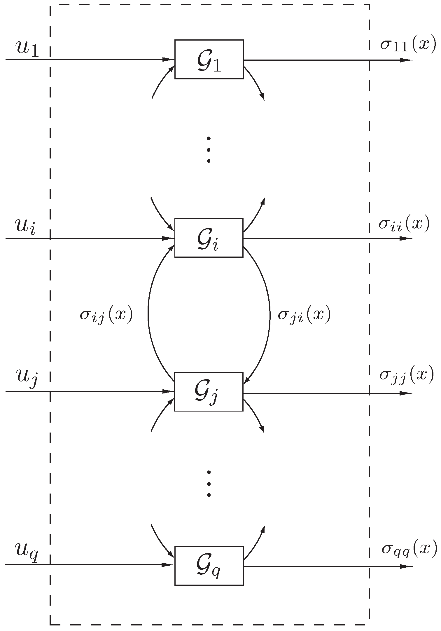