Some Further Results on the Minimum Error Entropy Estimation


1
Department of Precision Instruments and Mechanology, Tsinghua University, Beijing, 100084, China
2
Department of Electrical and Computer Engineering, University of Florida, Gainesville, FL 32611, USA
*
Author to whom correspondence should be addressed.
Entropy 2012, 14(5), 966-977; https://doi.org/10.3390/e14050966
Submission received: 1 April 2012
/
Revised: 2 May 2012
/
Accepted: 10 May 2012
/
Published: 21 May 2012
Abstract
:The minimum error entropy (MEE) criterion has been receiving increasing attention due to its promising perspectives for applications in signal processing and machine learning. In the context of Bayesian estimation, the MEE criterion is concerned with the estimation of a certain random variable based on another random variable, so that the error’s entropy is minimized. Several theoretical results on this topic have been reported. In this work, we present some further results on the MEE estimation. The contributions are twofold: (1) we extend a recent result on the minimum entropy of a mixture of unimodal and symmetric distributions to a more general case, and prove that if the conditional distributions are generalized uniformly dominated (GUD), the dominant alignment will be the MEE estimator; (2) we show by examples that the MEE estimator (not limited to singular cases) may be non-unique even if the error distribution is restricted to zero-mean (unbiased).
MSC Codes:
62B101. Introduction
A central concept in information theory is entropy, which is a mathematical measure of the uncertainty or the amount of missing information [1]. Entropy has been widely used in many areas, including physics, mathematics, communication, economics, signal processing, machine learning, etc. The maximum entropy principle is a powerful and widely accepted method for statistical inference or probabilistic reasoning with incomplete knowledge of probability distribution [2]. Another important entropy principle is the minimum entropy principle, which decreases the uncertainty associated with a system. In particular, the minimum error entropy (MEE) criterion can be applied in problems like estimation [3,4,5], identification [6,7], filtering [8,9,10], and system control [11,12]. In recent years, the MEE criterion, together with the nonparametric Renyi entropy estimator, has been successfully used in information theoretic learning (ITL) [13,14,15].
In the scenario of Bayesian estimation, the MEE criterion aims to minimize the entropy of the estimation error, and hence decrease the uncertainty in estimation. Given two random variables:
, an unknown parameter to be estimated, and
, the observation (or measurement), the MEE estimation of
based on can be formulated as:
where
denotes an estimator of
based on
, is a measurable function,
stands for the collection of all measurable functions of
,
denotes the Shannon entropy of the estimation error
, and
denotes the probability density function (PDF) of the estimation error. Let
be the conditional PDF of
given
. Then:
where
denotes the distribution function of
. From (2), one can see the error PDF
is actually a mixture of the shifted conditional PDF.
Different from conventional Bayesian risks, like mean square error (MSE) and risk-sensitive cost [16], the “loss function” in MEE is
, which is directly related to the error’s PDF, transforming nonlinearly the error by its own PDF. Some theoretical aspects of MEE estimation have been studied in the literature. In an early work [3], Weidemann and Stear proved that minimizing the error entropy is equivalent to minimizing the mutual information between the error and the observation, and also proved that the reduced error entropy is upper-bounded by the amount of information obtained by the observation. In [17], Janzura et al. proved that, for the case of finite mixtures (
is a discrete random variable with finite possible values), the MEE estimator equals the conditional median provided that the conditional PDFs are conditionally symmetric and unimodal (CSUM). Otahal [18] extended Janzura’s results to finite-dimensional Euclidean space. In a recent paper, Chen and Geman [19] employed a “function rearrangement” to study the minimum entropy of a mixture of CSUM distributions where no restriction on
was imposed. More recently, Chen et al. have investigated the robustness, non-uniqueness (for singular cases), sufficient condition, and the necessary condition involved in the MEE estimation [20]. Chen et al. have also presented a new interpretation on the MSE criterion as a robust MEE criterion [21].
In this work, we continue the study on the MEE estimation, and obtain some further results. Our contributions are twofold. First, we extend the results of Chen and Geman to a more general case, and show that when the conditional PDFs are generalized uniformly dominated (GUD), the MEE estimator equals the dominant alignment. Second, we show by examples that, the unbiased MEE estimator (not limited to singular cases) may be non-unique, and there can even be infinitely many optimal solutions. The rest of the paper is organized as follows. In Section 2, we study the minimum entropy of a mixture of generalized uniformly dominated conditional distributions. In Section 3, we present two examples to show the non-uniqueness of the unbiased MEE estimation. Finally, we give our conclusions in Section 4.
2. MEE Estimator for Generalized Uniformly Dominated Conditional Distributions
Before presenting the main theorem of this section, we give the following definitions.
Definition 1: Let
be a set of nonnegative, integrable functions, where
denotes an index set (possibly uncountable). Then
is said to be uniformly dominated in
if and only if
, there exists a measurable set
, satisfying
and:
where
is Lebesgue measure. The set
is called the
-volume dominant support of
.
Definition 2: The nonnegative, integrable function set
is said to be generalized uniformly dominated (GUD) in
if and only if there exists a function
, such that
is uniformly dominated, where:
The function
is called the dominant alignment of
.
Remark 1: The dominant alignment is, obviously, non-unique. If
is a dominant alignment of
, then
,
will also be a dominant alignment of
.
When regarding
as an index parameter, the conditional PDF
will represent a set of nonnegative and integrable functions, that is:
If the above function set is (generalized) uniformly dominated in
, then we say that the conditional PDF
is (generalized) uniformly dominated in
.
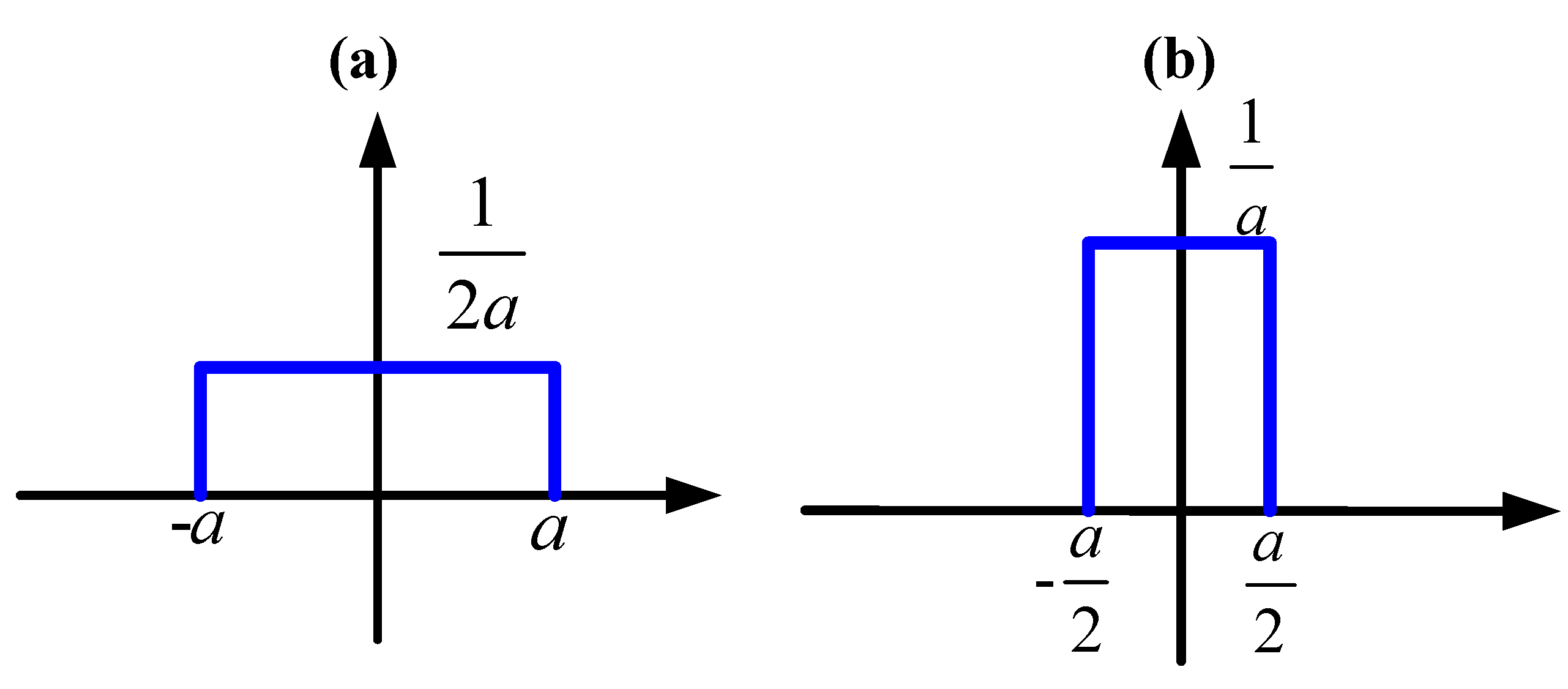
Remark 2: The GUD is much more general than CSUM. Actually, if the conditional PDF is CSUM, it must also be GUD (with the conditional mean as the dominant alignment), but not vice versa. In Figure 1 we show two examples where two PDFs (solid and dotted lines) are uniformly dominated but not CSUM.
Figure 1.
Uniformly dominated PDFs: (a) non-symmetric, (b) non-unimodal.
Theorem 1: Assume the conditional PDF
is generalized uniformly dominated in
, with dominant alignment
. If
exists (here “exists” means “exists in the extended sense” as defined in [19]) then
for all
for which
also exists.
Proof of Theorem 1: The proof presented below is similar to that of the Theorem 1 in [19], except that the discretization procedure is avoided. In the following, we give a brief sketch of the proof, and consider only the case
(the proof can be easily extended to
). First, one needs to prove the following proposition.
Proposition 1: Assume that the function
, ,
(not necessarily a conditional PDF) satisfies the following conditions:
- (1)
- non-negative, continuous, and integrable in for each ;
- (2)
- generalized uniformly dominated in , with dominant alignment ;
- (3)
- uniformly bounded in .
Then for any
, we have:
where
(here we extend the entropy definition to nonnegative
functions), and:
Remark 3: It is easy to verify that
(not necessarily
).
Proof of Proposition 1: The above proposition can be readily proved using the following two lemmas.
Lemma 1 [19]: Assume the nonnegative function
is bounded, continuous, and integrable, and define the function
by (
is Lebesgue measure):
Then the following results hold:
- (a)
- Define , , and . Then is continuous and non-increasing on , and as .
- (b)
- For any function with
- (c)
- For any
Proof of Lemma 1: See [19].
Remark 4: Denote
, and
. Then by Lemma 1, we have
and
(let ). Therefore, to prove Proposition 1, it suffices to prove:
Lemma 2: Functions and satisfy:
- (a)
- (b)
Proof of Lemma 2: (a) comes directly from the fact
. We only need to prove (b). We have:
where
is the
-volume dominant support of
. By Lemma 1 (c):
Thus , we have :
We are now in position to prove (11):
where
denotes the indicator function, and (a) follows from
, , that is:
In the above proof, we adopt the convention
.
Now the proof of Proposition 1 has been completed. To finish the proof of Theorem 1, we have to remove the conditions of continuity and uniform boundedness imposed in Proposition 1. This can be easily accomplished by approximating
by a sequence of functions
, , which satisfy these conditions. The remaining proof is omitted here, since it is exactly the same as the last part of the proof for Theorem 1 in [19].
Example 1: Consider an additive noise model:
where
is an additive noise that is independent of
. In this case, we have
, where
denotes the noise PDF. It is clear that
is generalized uniformly dominated, with dominant alignment
. According to Theorem 1, we have
. In fact, this result can also be proved by:
where (b) comes from the fact that
and
are independent (For independent random variables
and , the inequality
holds). In this example, the conditional PDF
is, obviously, not necessarily CSUM.
Example 2: Suppose the joint PDF of random variables
,
() is:
where
,
. Then the conditional PDF
will be:
One can easily verify that the above conditional PDF is non-symmetric but generalized uniformly dominated, with dominant alignment
(the ε-volume dominant support of
is
). By Theorem 1, the function
is the minimizer of error entropy.
3. Non-Uniqueness of Unbiased MEE Estimation
Because entropy is shift-invariant, the MEE estimator is obviously non-unique. In practical applications, in order to yield a unique solution, or to meet the desire for small error values, the MEE estimator is usually restricted to be unbiased, that is, the estimation error is restricted to be zero-mean [15]. The question of interest in this paper is whether the unbiased MEE estimator is unique. In [20], it has been shown that, for the singular case (in which the error entropy approaches minus infinity), the unbiased MEE estimation may yield non-unique (even infinitely many) solutions. In the following, we present two examples to show that this result still holds even for nonsingular case.
Example 3: Let the joint PDF of
and
() be a mixed-Gaussian density [20]:
where
,
. The conditional PDF of
given
will be:
,
is symmetric around zero (but not unimodal in x). It can be shown that for some values of
, , the MEE estimator of
based on
does not equal zero (see [20], Example 3). In these cases, the MEE estimator will be non-unique, even if the error’s PDF is restricted to zero-mean (unbiased) distribution. This can be proved as follows:
Let
be an unbiased MEE estimator of
based on
. Then
will also be an unbiased MEE estimator, because:
where (c) comes from the fact that
is symmetric around zero, and further:
If the unbiased MEE estimator is unique, then we have
, which contradicts the fact that
does not equal zero. Therefore, the unbiased MEE estimator must be non-unique. Obviously, the above result can be extended to more general cases. In fact, we have the following proposition.
Proposition2: The unbiased MEE estimator will be non-unique if the conditional PDF
satisfies:
- (1)
- Symmetric in around the conditional mean for each ;
- (2)
- There exists a function such that , .
Proof: Similar to the proof presented above (Omitted).
In the next example, we show that, for some particular situations, there can be even infinitely many unbiased MEE estimators.
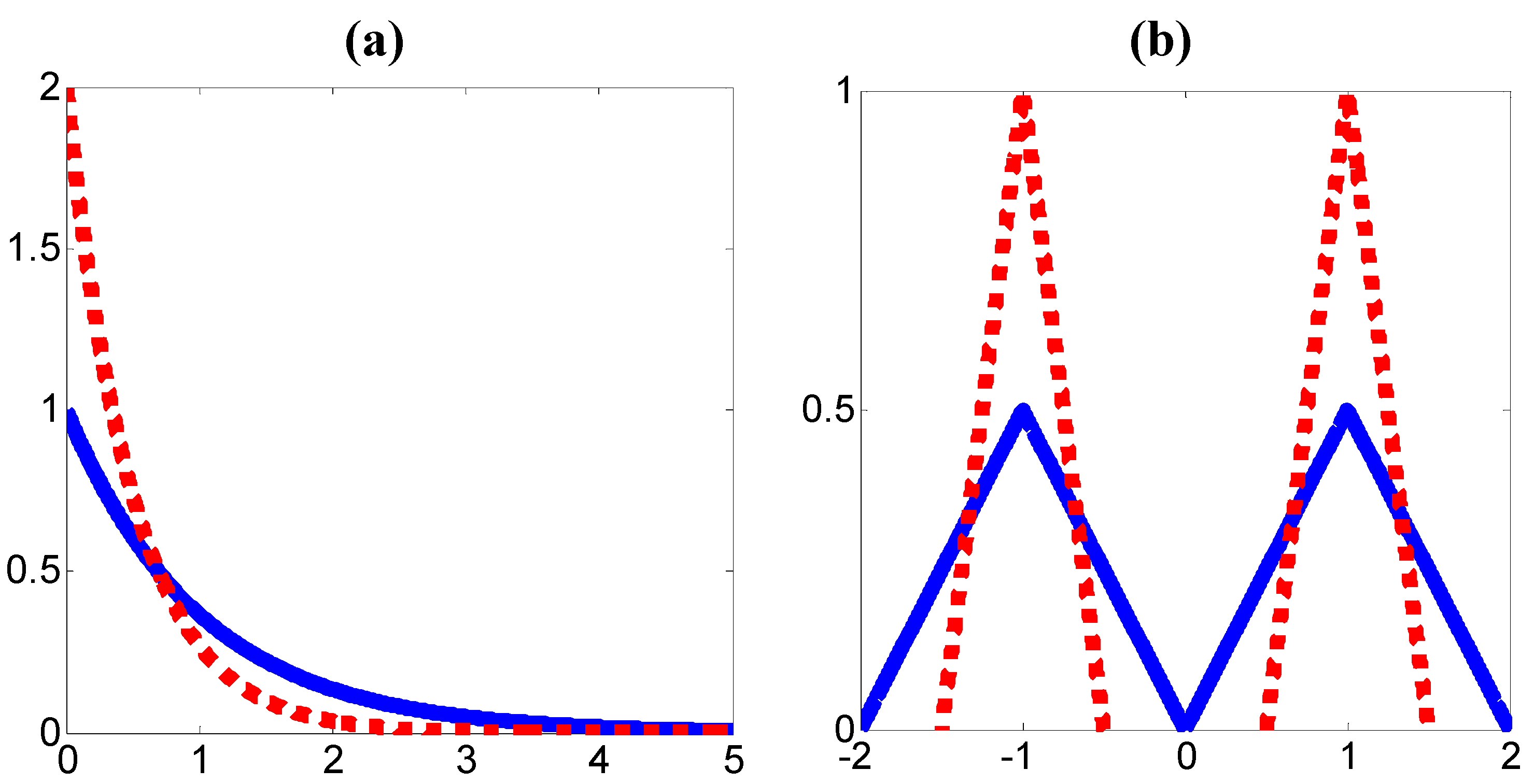
Example 4: Suppose is a discrete random variable with Bernoulli distribution:
The conditional PDF of
given
is (see Figure 2):
where
. Note that the above conditional PDF is uniformly dominated in
.
Figure 2.
Conditional PDF of given : (a) , (b) .

Given an estimator
, the error’s PDF will be:
Let be an unbiased estimator, then
, and hence
. In the following, we assume
(due to symmetry, one can obtain similar results for
), and consider three cases:
Case 1:
. In this case, the error PDF is:
Then the error entropy can be calculated as:
Case 2:
. In this case, we have:
And hence:
Case 3:
. In this case:
Thus:
One can easily verify that the error entropy achieves its minimum value when
(the first case). There are, therefore, infinitely many unbiased estimators that minimize the error entropy.
4. Conclusion
Two issues involved in the minimum error entropy (MEE) estimation have been studied in this work. The first issue is about which estimator minimizes the error entropy. In general there is no explicit expression for the MEE estimator unless some constraints on the conditional distribution are imposed. In the past, several researchers have shown that, if the conditional density is conditionally symmetric and unimodal (CSUM), then the conditional mean (or median) will be the MEE estimator. We extend these results to a more general case, and show that if the conditional densities are generalized uniformly dominated (GUD), then the dominant alignment will minimize the error entropy. The second issue is about the non-uniqueness of the unbiased MEE estimation. It has been shown in a recent paper that for the singular case (in which the error entropy approaches minus infinity), the unbiased MEE estimation may yield non-unique (even infinitely many) solutions. In this work, we show by examples that this result still holds even for nonsingular case.
Acknowledgments
This work was supported by National Natural Science Foundation of China (No. 60904054), NSF grant ECCS 0856441, and ONR N00014-10-1-0375.
References
- Cover, T.M.; Thomas, J.A. Element of Information Theory; Wiley & Son, Inc.: New York, NY, USA, 1991. [Google Scholar]
- Kapur, J.N.; Kesavan, H.K. Entropy Optimization Principles with Applications; Academic Press, Inc.: Boston, MA, USA, 1992. [Google Scholar]
- Weidemann, H.L.; Stear, E.B. Entropy analysis of estimating systems. IEEE Trans. Inform. Theor. 1970, 16, 264–270. [Google Scholar] [CrossRef]
- Tomita, Y.; Ohmatsu, S.; Soeda, T. An application of the information theory to estimation problems. Inf. Control 1976, 32, 101–111. [Google Scholar] [CrossRef]
- Wolsztynski, E.; Thierry, E.; Pronzato, L. Minimum-entropy estimation in semiparametric models. Signal Process. 2005, 85, 937–949. [Google Scholar] [CrossRef]
- Guo, L.Z.; Billings, S.A.; Zhu, D.Q. An extended orthogonal forward regression algorithm for system identification using entropy. Int. J. Control 2008, 81, 690–699. [Google Scholar] [CrossRef]
- Chen, B.; Zhu, Y.; Hu, J.; Principe, J.C. △-entropy: Definition, properties and applications in system identification with quantized data. Inf. Sci. 2011, 181, 1384–1402. [Google Scholar] [CrossRef]
- Kalata, P.; Priemer, R. Linear prediction, filtering and smoothing: an information theoretic approach. Inf. Sci. 1979, 17, 1–14. [Google Scholar] [CrossRef]
- Feng, X.; Loparo, K.A.; Fang, Y. Optimal state estimation for stochastic systems: An information theoretic approach. IEEE Trans. Automat. Contr. 1997, 42, 771–785. [Google Scholar] [CrossRef]
- Guo, L.; Wang, H. Minimum entropy filtering for multivariate stochastic systems with non-Gaussian Noises. IEEE Trans. Autom. Control 2006, 51, 695–700. [Google Scholar] [CrossRef]
- Wang, H. Minimum entropy control of non-Gaussian dynamic stochastic systems. IEEE Trans. Autom. Control 2002, 47, 398–403. [Google Scholar] [CrossRef]
- Yue, H.; Wang, H. Minimum entropy control of closed-loop tracking errors for dynamic stochastic systems. IEEE Trans. Autom. Control 2003, 48, 118–122. [Google Scholar]
- Erdogmus, D.; Principe, J.C. An error-entropy minimization algorithm for supervised training of nonlinear adaptive systems. IEEE Trans. Signal Process. 2002, 50, 1780–1786. [Google Scholar] [CrossRef]
- Erdogmus, D.; Principe, J.C. From linear adaptive filtering to nonlinear information processing—The design and analysis of information processing systems. IEEE Signal Process. Mag. 2006, 23, 14–33. [Google Scholar] [CrossRef]
- Principe, J.C. Information Theoretic Learning: Renyi's Entropy and Kernel Perspectives; Springer: New York, NY, USA, 2010. [Google Scholar]
- Boel, R.K.; James, M.R.; Petersen, I.R. Robustness and risk-sensitive filtering. IEEE Trans. Autom. Control 2002, 47, 451–461. [Google Scholar] [CrossRef]
- Janzura, M.; Koski, T.; Otahal, A. Minimum entropy of error principle in estimation. Inf. Sci. 1994, 79, 123–144. [Google Scholar] [CrossRef]
- Otahal, A. Minimum entropy of error estimate for multi-dimensional parameter and finite-state-space observations. Kybernetika 1995, 31, 331–335. [Google Scholar]
- Chen, T.-L.; Geman, S. On the minimum entropy of a mixture of unimodal and symmetric distributions. IEEE Trans. Inf. Theory 2008, 54, 3166–3174. [Google Scholar] [CrossRef]
- Chen, B.; Zhu, Y.; Hu, J.; Zhang, M. On optimal estimations with minimum error entropy criterion. J. Frankl. Inst.-Eng. Appl. Math. 2010, 347, 545–558. [Google Scholar] [CrossRef]
- Chen, B.; Zhu, Y.; Hu, J.; Zhang, M. A new interpretation on the MMSE as a robust MEE criterion. Signal Process. 2010, 90, 3313–3316. [Google Scholar] [CrossRef]
© 2012 by the authors; licensee MDPI, Basel, Switzerland. This article is an open access article distributed under the terms and conditions of the Creative Commons Attribution license (http://creativecommons.org/licenses/by/3.0/).
Share and Cite
MDPI and ACS Style
Chen, B.; Principe, J.C. Some Further Results on the Minimum Error Entropy Estimation. Entropy 2012, 14, 966-977. https://doi.org/10.3390/e14050966
AMA Style
Chen B, Principe JC. Some Further Results on the Minimum Error Entropy Estimation. Entropy. 2012; 14(5):966-977. https://doi.org/10.3390/e14050966
Chicago/Turabian StyleChen, Badong, and Jose C. Principe. 2012. "Some Further Results on the Minimum Error Entropy Estimation" Entropy 14, no. 5: 966-977. https://doi.org/10.3390/e14050966