4.1. Monte Carlo Design
The Monte Carlo experiments are constructed in the following manner: three different sample sizes were analyzed, namely,
n = 25, 60, and 90. For each sample size, three different specifications of spatial weight matrices were used. Weight matrices differ in their degree of sparseness, they have equal weights, and an average number of neighbors per unit,
J, is chosen to be
J = 2, 6 and 10 [
50]. Eleven values for the spatial autoregressive coefficient
ρ in (1) are chosen, namely, −0.9, −0.8, −0.6, −0.4, −0.2, 0, 0.2, 0.4, 0.6, 0.8 and 0.9. Three values of
are 1, 2.5, and 5. The remaining elements of the parameter vector are specified as
. Two regressors,
, are specified as
~
and
~
. The
n observations on independent variables are normalized so that their sample means and variances are, respectively, zero and one. The same regressors are used in all experiments and 1000 repetitions were conducted for each Monte Carlo experiment. In summary, there are then three values of
n, eleven values of ρ, three values of
, and three values of
J. All combinations of
n, ρ,
, and
J result in 3 × 11 × 3 × 3 = 297 Monte Carlo experiments.
In addition, three different parametric functional forms for the distribution of the disturbance term ε in (1) are analyzed, together with varying specifications relating to heteroskedasticity. First, normally distributed homoscedastic disturbance terms, ~ for ∀i = 1,…,n, are considered and referred to as H = 1. Three forms of heteroscedasticity are also specified for the normal distribution such that , , and , referred to as H = 2, H = 3, H = 4, correspondingly. In addition, the log-normal distribution (H = 5) is chosen because of its asymmetric nature such that , where ~ . Finally, a mixture of normal is considered (H = 6), where a normally distributed variable is contaminated by another with a larger variance, producing thicker tails than a normal distribution, i.e., , the are iid Bernoulli variables with , ~ and ~ . There are 297 experiments for the 6 distributional assumptions considered, which result in a total of 297 × 6 = 1782 Monte Carlo experiments performed.
To keep the Monte Carlo study manageable in terms of reporting results, bias and spread of the estimator distributions are measured by root mean square error (RMSE). Since sample moments for the calculation of the standard RMSE might not exist, the RMSE’s measure proposed by [
50] is used, which guarantees the existence of necessary components. According to Kelejian and Prucha [
48],
where the
bias is the difference between the median and the true parameter values, and
is the inter-quantile range where
and
are 0.75 and 0.25 quantiles, correspondingly.
In addition, response functions are used to summarize the relationship between RMSEs of estimators and model parameters over the set of all considered parameter values. In particular, let
,
,
,
and
be the values, respectively, of ρ,
,
,
J and
in the
ith experiment,
i = 1,…,297, for each distributional assumption, and let
correspond to the sample size. Then the functional form of the response function [
51] is:
where
RMSEi is the RMSE of an estimator of a given parameter in the
ith experiment and the parameters
are different for each estimator of each parameter. For each case considered, the parameters of (22) are estimated using the entire set of 297 Monte Carlo experiments for each distributional assumption by least squares after taking natural logs on both sides.
4.2. Results
There are three types of results presented. First, tables of root mean square errors of the estimators for a subset of experiments are reported. Second, average RMSEs for the entire Monte Carlo study are provided. Finally, response functions for the RMSEs of estimators are estimated, and graphs of these response functions are presented.
In order to conserve space,
Table 1,
Table 2 and
Table 3 report RMSEs of the estimators for a selected subset of experimental parameter values. These tables report RMSEs of the estimators of the parameters
,
and
, correspondingly, for 33 Monte Carlo experiments representing a combination of 11 parameter values for ρ and 3 parameter values for
, with the average number of neighbors
J = 6, sample size
n = 60, and normally distributed disturbance term
H = 1.
According to
Table 1, the RMSEs of the QML estimator of ρ are the lowest and the OLS estimator are the largest, since the OLS estimator is inconsistent and the QML estimator with a normally distributed homoscedastic disturbance term is consistent and efficient.
Table 1.
Root mean square errors of estimators of ρ, n = 60, J = 6, H = 1.
Table 1.
Root mean square errors of estimators of ρ, n = 60, J = 6, H = 1.
| ρ | | OLS | 2SLS | GMM | QML | MEEL | MEL | MLEL |
|---|
| 0.9 | 1 | 0.055 | 0.048 | 0.048 | 0.036 | 0.051 | 0.074 | 0.051 |
| 0.9 | 2.5 | 0.077 | 0.061 | 0.063 | 0.040 | 0.065 | 0.093 | 0.069 |
| 0.9 | 5 | 0.110 | 0.115 | 0.111 | 0.046 | 0.113 | 0.098 | 0.127 |
| 0.8 | 1 | 0.077 | 0.069 | 0.070 | 0.055 | 0.071 | 0.120 | 0.074 |
| 0.8 | 2.5 | 0.155 | 0.128 | 0.138 | 0.073 | 0.143 | 0.121 | 0.153 |
| 0.8 | 5 | 0.189 | 0.178 | 0.183 | 0.079 | 0.165 | 0.146 | 0.180 |
| 0.6 | 1 | 0.173 | 0.148 | 0.159 | 0.097 | 0.149 | 0.116 | 0.155 |
| 0.6 | 2.5 | 0.237 | 0.227 | 0.233 | 0.113 | 0.236 | 0.133 | 0.243 |
| 0.6 | 5 | 0.258 | 0.236 | 0.260 | 0.124 | 0.258 | 0.146 | 0.267 |
| 0.4 | 1 | 0.159 | 0.166 | 0.170 | 0.116 | 0.160 | 0.128 | 0.166 |
| 0.4 | 2.5 | 0.229 | 0.241 | 0.245 | 0.139 | 0.247 | 0.157 | 0.251 |
| 0.4 | 5 | 0.271 | 0.295 | 0.288 | 0.150 | 0.267 | 0.181 | 0.274 |
| 0.2 | 1 | 0.196 | 0.194 | 0.204 | 0.137 | 0.200 | 0.190 | 0.207 |
| 0.2 | 2.5 | 0.260 | 0.295 | 0.294 | 0.153 | 0.276 | 0.222 | 0.289 |
| 0.2 | 5 | 0.315 | 0.400 | 0.389 | 0.216 | 0.354 | 0.233 | 0.369 |
| 0 | 1 | 0.204 | 0.209 | 0.214 | 0.153 | 0.210 | 0.164 | 0.219 |
| 0 | 2.5 | 0.305 | 0.315 | 0.331 | 0.201 | 0.302 | 0.220 | 0.310 |
| 0 | 5 | 0.389 | 0.563 | 0.593 | 0.220 | 0.506 | 0.255 | 0.532 |
| −0.2 | 1 | 0.231 | 0.213 | 0.225 | 0.166 | 0.205 | 0.184 | 0.207 |
| −0.2 | 2.5 | 0.404 | 0.390 | 0.414 | 0.219 | 0.389 | 0.238 | 0.397 |
| −0.2 | 5 | 0.424 | 0.465 | 0.496 | 0.216 | 0.393 | 0.274 | 0.410 |
| −0.4 | 1 | 0.360 | 0.282 | 0.321 | 0.200 | 0.284 | 0.230 | 0.288 |
| −0.4 | 2.5 | 0.476 | 0.421 | 0.438 | 0.214 | 0.405 | 0.256 | 0.415 |
| −0.4 | 5 | 0.555 | 0.556 | 0.612 | 0.232 | 0.533 | 0.328 | 0.533 |
| −0.6 | 1 | 0.360 | 0.256 | 0.282 | 0.193 | 0.242 | 0.221 | 0.246 |
| −0.6 | 2.5 | 0.581 | 0.434 | 0.497 | 0.240 | 0.397 | 0.315 | 0.408 |
| −0.6 | 5 | 0.669 | 0.598 | 0.627 | 0.239 | 0.549 | 0.350 | 0.546 |
| −0.8 | 1 | 0.532 | 0.368 | 0.382 | 0.208 | 0.302 | 0.266 | 0.307 |
| −0.8 | 2.5 | 0.591 | 0.442 | 0.463 | 0.247 | 0.364 | 0.307 | 0.368 |
| −0.8 | 5 | 0.789 | 0.609 | 0.569 | 0.240 | 0.504 | 0.337 | 0.498 |
| −0.9 | 1 | 0.328 | 0.224 | 0.186 | 0.175 | 0.178 | 0.144 | 0.189 |
| −0.9 | 2.5 | 0.656 | 0.411 | 0.387 | 0.217 | 0.323 | 0.244 | 0.329 |
| −0.9 | 5 | 0.757 | 0.576 | 0.392 | 0.235 | 0.396 | 0.225 | 0.403 |
| Column Average | 0.345 | 0.307 | 0.312 | 0.163 | 0.280 | 0.203 | 0.287 |
Table 2.
Root mean square errors of estimators of , n = 60, J = 6, H = 1.
Table 2.
Root mean square errors of estimators of , n = 60, J = 6, H = 1.
| ρ | | OLS | 2SLS | GMM | QML | MEEL | MEL | MLEL |
|---|
| 0.9 | 1 | 0.141 | 0.142 | 0.141 | 0.139 | 0.142 | 0.154 | 0.146 |
| 0.9 | 2.5 | 0.217 | 0.217 | 0.219 | 0.222 | 0.221 | 0.247 | 0.224 |
| 0.9 | 5 | 0.294 | 0.309 | 0.313 | 0.303 | 0.315 | 0.334 | 0.312 |
| 0.8 | 1 | 0.132 | 0.131 | 0.132 | 0.128 | 0.137 | 0.151 | 0.138 |
| 0.8 | 2.5 | 0.225 | 0.228 | 0.229 | 0.222 | 0.221 | 0.254 | 0.228 |
| 0.8 | 5 | 0.301 | 0.312 | 0.315 | 0.293 | 0.307 | 0.321 | 0.304 |
| 0.6 | 1 | 0.132 | 0.133 | 0.135 | 0.130 | 0.136 | 0.175 | 0.137 |
| 0.6 | 2.5 | 0.206 | 0.209 | 0.209 | 0.203 | 0.202 | 0.249 | 0.208 |
| 0.6 | 5 | 0.305 | 0.299 | 0.300 | 0.293 | 0.305 | 0.346 | 0.310 |
| 0.4 | 1 | 0.129 | 0.130 | 0.129 | 0.129 | 0.135 | 0.192 | 0.134 |
| 0.4 | 2.5 | 0.204 | 0.206 | 0.206 | 0.202 | 0.204 | 0.272 | 0.209 |
| 0.4 | 5 | 0.303 | 0.305 | 0.316 | 0.304 | 0.310 | 0.351 | 0.306 |
| 0.2 | 1 | 0.130 | 0.134 | 0.135 | 0.128 | 0.135 | 0.190 | 0.139 |
| 0.2 | 2.5 | 0.217 | 0.219 | 0.220 | 0.219 | 0.223 | 0.262 | 0.221 |
| 0.2 | 5 | 0.295 | 0.305 | 0.314 | 0.302 | 0.314 | 0.356 | 0.319 |
| 0 | 1 | 0.133 | 0.136 | 0.137 | 0.129 | 0.144 | 0.171 | 0.146 |
| 0 | 2.5 | 0.211 | 0.209 | 0.213 | 0.211 | 0.210 | 0.252 | 0.210 |
| 0 | 5 | 0.296 | 0.309 | 0.320 | 0.294 | 0.315 | 0.339 | 0.315 |
| −0.2 | 1 | 0.126 | 0.129 | 0.127 | 0.126 | 0.132 | 0.165 | 0.142 |
| −0.2 | 2.5 | 0.199 | 0.202 | 0.203 | 0.201 | 0.199 | 0.236 | 0.204 |
| −0.2 | 5 | 0.297 | 0.305 | 0.302 | 0.307 | 0.320 | 0.341 | 0.318 |
| −0.4 | 1 | 0.139 | 0.142 | 0.145 | 0.137 | 0.142 | 0.197 | 0.144 |
| −0.4 | 2.5 | 0.205 | 0.212 | 0.222 | 0.208 | 0.207 | 0.259 | 0.215 |
| −0.4 | 5 | 0.295 | 0.292 | 0.303 | 0.282 | 0.299 | 0.334 | 0.299 |
| −0.6 | 1 | 0.131 | 0.130 | 0.130 | 0.129 | 0.131 | 0.185 | 0.137 |
| −0.6 | 2.5 | 0.240 | 0.224 | 0.234 | 0.220 | 0.223 | 0.281 | 0.223 |
| −0.6 | 5 | 0.303 | 0.317 | 0.314 | 0.296 | 0.317 | 0.333 | 0.323 |
| −0.8 | 1 | 0.142 | 0.134 | 0.139 | 0.136 | 0.140 | 0.180 | 0.140 |
| −0.8 | 2.5 | 0.216 | 0.219 | 0.236 | 0.210 | 0.219 | 0.276 | 0.219 |
| −0.8 | 5 | 0.293 | 0.298 | 0.312 | 0.290 | 0.301 | 0.317 | 0.309 |
| −0.9 | 1 | 0.142 | 0.129 | 0.132 | 0.126 | 0.134 | 0.175 | 0.137 |
| −0.9 | 2.5 | 0.237 | 0.214 | 0.225 | 0.209 | 0.211 | 0.274 | 0.218 |
| −0.9 | 5 | 0.285 | 0.294 | 0.307 | 0.284 | 0.300 | 0.337 | 0.295 |
| Column Average | 0.216 | 0.217 | 0.222 | 0.213 | 0.220 | 0.258 | 0.222 |
This is not surprising since in this case, the QML estimator is actually a correctly specified classical ML estimator. The IT estimators of ρ have the second lowest RMSEs, outperforming the OLS, 2SLS, and GMM estimators. The MEL estimator outperforms the other IT estimators but is, on average, slightly less efficient than the QML estimator.
Table 2 and
Table 3 report the RMSEs of the QML and IT estimators of
and
which are on average roughly the same. A loss of efficiency of the IT estimators relative to the QML estimators is small and mostly arises from estimation of the spatial autocorrelation coefficient ρ [
11]. The same pattern holds for other distributional assumptions, namely
H = 2,...,5, and only the averages of the RMSEs are reported.
In order to summarize the results of the total 1782 Monte Carlo experiments, average RMSEs of the estimators, namely, for ρ,
and
, are presented in
Table 4,
Table 5,
Table 6,
Table 7,
Table 8 and
Table 9. A table’s entry is the averages of RMSEs of estimators over 33 Monte Carlo experiments for a given sample size
n, average number of neighbors
J, and distributional assumptions
H.
Table 3.
Root mean square errors of estimators of , n = 60, J = 6, H = 1.
Table 3.
Root mean square errors of estimators of , n = 60, J = 6, H = 1.
| ρ | | OLS | 2SLS | GMM | QML | MEEL | MEL | MLEL |
|---|
| 0.9 | 1 | 0.131 | 0.130 | 0.131 | 0.126 | 0.139 | 0.149 | 0.141 |
| 0.9 | 2.5 | 0.233 | 0.236 | 0.243 | 0.230 | 0.246 | 0.249 | 0.243 |
| 0.9 | 5 | 0.297 | 0.307 | 0.308 | 0.301 | 0.314 | 0.330 | 0.310 |
| 0.8 | 1 | 0.140 | 0.137 | 0.143 | 0.136 | 0.141 | 0.156 | 0.146 |
| 0.8 | 2.5 | 0.225 | 0.225 | 0.239 | 0.221 | 0.237 | 0.244 | 0.237 |
| 0.8 | 5 | 0.274 | 0.278 | 0.277 | 0.275 | 0.292 | 0.306 | 0.293 |
| 0.6 | 1 | 0.127 | 0.125 | 0.124 | 0.125 | 0.128 | 0.173 | 0.132 |
| 0.6 | 2.5 | 0.199 | 0.198 | 0.199 | 0.204 | 0.205 | 0.249 | 0.214 |
| 0.6 | 5 | 0.301 | 0.311 | 0.308 | 0.302 | 0.304 | 0.345 | 0.307 |
| 0.4 | 1 | 0.137 | 0.132 | 0.131 | 0.133 | 0.137 | 0.186 | 0.140 |
| 0.4 | 2.5 | 0.211 | 0.215 | 0.219 | 0.210 | 0.226 | 0.265 | 0.226 |
| 0.4 | 5 | 0.299 | 0.303 | 0.312 | 0.312 | 0.311 | 0.340 | 0.316 |
| 0.2 | 1 | 0.135 | 0.136 | 0.137 | 0.134 | 0.140 | 0.182 | 0.144 |
| 0.2 | 2.5 | 0.219 | 0.224 | 0.224 | 0.221 | 0.220 | 0.269 | 0.226 |
| 0.2 | 5 | 0.308 | 0.309 | 0.314 | 0.306 | 0.319 | 0.334 | 0.321 |
| 0 | 1 | 0.131 | 0.132 | 0.131 | 0.133 | 0.140 | 0.179 | 0.141 |
| 0 | 2.5 | 0.228 | 0.230 | 0.227 | 0.226 | 0.233 | 0.259 | 0.236 |
| 0 | 5 | 0.290 | 0.302 | 0.304 | 0.292 | 0.304 | 0.333 | 0.309 |
| −0.2 | 1 | 0.128 | 0.128 | 0.131 | 0.126 | 0.141 | 0.182 | 0.147 |
| −0.2 | 2.5 | 0.205 | 0.210 | 0.208 | 0.206 | 0.221 | 0.251 | 0.221 |
| −0.2 | 5 | 0.282 | 0.302 | 0.303 | 0.281 | 0.296 | 0.310 | 0.306 |
| −0.4 | 1 | 0.134 | 0.137 | 0.135 | 0.133 | 0.141 | 0.178 | 0.143 |
| −0.4 | 2.5 | 0.216 | 0.217 | 0.221 | 0.214 | 0.222 | 0.250 | 0.230 |
| −0.4 | 5 | 0.302 | 0.300 | 0.312 | 0.294 | 0.312 | 0.331 | 0.319 |
| −0.6 | 1 | 0.133 | 0.131 | 0.131 | 0.126 | 0.140 | 0.179 | 0.142 |
| −0.6 | 2.5 | 0.236 | 0.214 | 0.212 | 0.202 | 0.214 | 0.257 | 0.213 |
| −0.6 | 5 | 0.316 | 0.321 | 0.336 | 0.298 | 0.314 | 0.361 | 0.318 |
| −0.8 | 1 | 0.156 | 0.149 | 0.155 | 0.142 | 0.147 | 0.190 | 0.148 |
| −0.8 | 2.5 | 0.227 | 0.212 | 0.234 | 0.212 | 0.222 | 0.269 | 0.218 |
| −0.8 | 5 | 0.311 | 0.324 | 0.320 | 0.308 | 0.324 | 0.343 | 0.315 |
| −0.9 | 1 | 0.137 | 0.137 | 0.139 | 0.136 | 0.140 | 0.192 | 0.145 |
| −0.9 | 2.5 | 0.216 | 0.199 | 0.205 | 0.200 | 0.213 | 0.265 | 0.212 |
| −0.9 | 5 | 0.305 | 0.327 | 0.342 | 0.296 | 0.330 | 0.360 | 0.344 |
| Column Average | 0.218 | 0.219 | 0.223 | 0.214 | 0.225 | 0.257 | 0.227 |
The results of the Monte Carlo experiments for other distributional assumptions are consistent with the results for a subset of parameter space for the case of
H = 1 reported in
Table 1,
Table 2 and
Table 3. In fact,
Table 4 and
Table 5 indicate that the RMSEs of the QML estimator of ρ are the lowest, regardless of sample size, average number of neighbors, and distributional assumptions considered. The IT estimators of ρ have the second lowest RMSEs across all Monte Carlo experiments, being less efficient than the QML estimator, but often outperforming OLS, 2SLS, and GMM estimators.
Table 6,
Table 7,
Table 8 and
Table 9 indicate that the RMSEs of QML and the IT estimators of
and
are roughly the same with the exception of the MEL estimator which is, on average, less efficient than the QML estimator for
and
. Indeed, many cases exist where IT estimators (e.g., MLEL) outperform QML. In any case, the loss of efficiency of the IT estimators relative to the QML estimator is, on average, small and mostly arises from estimation of the spatial autocorrelation coefficient ρ.
Table 4.
Average root mean square errors of estimators of for H = 1−3.
Table 4.
Average root mean square errors of estimators of for H = 1−3.
| H | J | n | OLS | 2SLS | GMM | QML | MEEL | MEL | MLEL |
|---|
| 1 | 2 | 25 | 0.212 | 0.221 | 0.247 | 0.115 | 0.210 | 0.191 | 0.223 |
| 1 | 2 | 60 | 0.170 | 0.140 | 0.148 | 0.077 | 0.139 | 0.112 | 0.146 |
| 1 | 2 | 90 | 0.156 | 0.113 | 0.118 | 0.060 | 0.113 | 0.097 | 0.117 |
| 1 | 6 | 25 | 0.493 | 0.522 | 0.540 | 0.272 | 0.456 | 0.402 | 0.465 |
| 1 | 6 | 60 | 0.345 | 0.307 | 0.312 | 0.163 | 0.280 | 0.203 | 0.287 |
| 1 | 6 | 90 | 0.301 | 0.251 | 0.256 | 0.132 | 0.230 | 0.159 | 0.236 |
| 1 | 10 | 25 | 0.693 | 0.721 | 0.698 | 0.372 | 0.598 | 0.524 | 0.610 |
| 1 | 10 | 60 | 0.463 | 0.440 | 0.466 | 0.226 | 0.413 | 0.284 | 0.418 |
| 1 | 10 | 90 | 0.400 | 0.351 | 0.352 | 0.180 | 0.319 | 0.208 | 0.325 |
| 2 | 2 | 25 | 0.114 | 0.106 | 0.114 | 0.077 | 0.106 | 0.113 | 0.109 |
| 2 | 2 | 60 | 0.082 | 0.066 | 0.069 | 0.050 | 0.065 | 0.070 | 0.065 |
| 2 | 2 | 90 | 0.080 | 0.057 | 0.058 | 0.038 | 0.055 | 0.061 | 0.056 |
| 2 | 6 | 25 | 0.260 | 0.262 | 0.276 | 0.189 | 0.244 | 0.240 | 0.246 |
| 2 | 6 | 60 | 0.197 | 0.170 | 0.177 | 0.120 | 0.154 | 0.145 | 0.154 |
| 2 | 6 | 90 | 0.162 | 0.125 | 0.133 | 0.095 | 0.117 | 0.116 | 0.117 |
| 2 | 10 | 25 | 0.395 | 0.422 | 0.435 | 0.273 | 0.370 | 0.360 | 0.370 |
| 2 | 10 | 60 | 0.272 | 0.244 | 0.257 | 0.189 | 0.225 | 0.214 | 0.224 |
| 2 | 10 | 90 | 0.225 | 0.184 | 0.196 | 0.133 | 0.169 | 0.156 | 0.169 |
| 3 | 2 | 25 | 0.148 | 0.134 | 0.140 | 0.081 | 0.126 | 0.144 | 0.127 |
| 3 | 2 | 60 | 0.143 | 0.117 | 0.117 | 0.061 | 0.106 | 0.111 | 0.105 |
| 3 | 2 | 90 | 0.132 | 0.099 | 0.104 | 0.046 | 0.084 | 0.093 | 0.083 |
| 3 | 6 | 25 | 0.365 | 0.375 | 0.386 | 0.217 | 0.336 | 0.341 | 0.334 |
| 3 | 6 | 60 | 0.285 | 0.240 | 0.257 | 0.134 | 0.207 | 0.217 | 0.203 |
| 3 | 6 | 90 | 0.269 | 0.236 | 0.246 | 0.115 | 0.203 | 0.178 | 0.197 |
| 3 | 10 | 25 | 0.444 | 0.473 | 0.510 | 0.277 | 0.418 | 0.425 | 0.420 |
| 3 | 10 | 60 | 0.367 | 0.336 | 0.360 | 0.183 | 0.300 | 0.288 | 0.294 |
| 3 | 10 | 90 | 0.325 | 0.325 | 0.343 | 0.146 | 0.260 | 0.241 | 0.253 |
Table 5.
Average root mean square errors of estimators of ρ for H = 4−6.
Table 5.
Average root mean square errors of estimators of ρ for H = 4−6.
| H | J | n | OLS | 2SLS | GMM | QML | MEEL | MEL | MLEL |
|---|
| 4 | 2 | 25 | 0.219 | 0.232 | 0.250 | 0.120 | 0.211 | 0.204 | 0.222 |
| 4 | 2 | 60 | 0.188 | 0.167 | 0.177 | 0.076 | 0.157 | 0.131 | 0.164 |
| 4 | 2 | 90 | 0.185 | 0.144 | 0.152 | 0.064 | 0.138 | 0.112 | 0.142 |
| 4 | 6 | 25 | 0.506 | 0.560 | 0.579 | 0.266 | 0.488 | 0.448 | 0.496 |
| 4 | 6 | 60 | 0.380 | 0.380 | 0.387 | 0.162 | 0.333 | 0.239 | 0.338 |
| 4 | 6 | 90 | 0.338 | 0.307 | 0.306 | 0.132 | 0.271 | 0.189 | 0.274 |
| 4 | 10 | 25 | 0.701 | 0.795 | 0.805 | 0.365 | 0.647 | 0.589 | 0.657 |
| 4 | 10 | 60 | 0.494 | 0.515 | 0.510 | 0.225 | 0.446 | 0.303 | 0.452 |
| 4 | 10 | 90 | 0.452 | 0.450 | 0.460 | 0.186 | 0.410 | 0.252 | 0.412 |
| 5 | 2 | 25 | 0.175 | 0.169 | 0.182 | 0.100 | 0.149 | 0.151 | 0.155 |
| 5 | 2 | 60 | 0.148 | 0.119 | 0.125 | 0.066 | 0.102 | 0.105 | 0.103 |
| 5 | 2 | 90 | 0.142 | 0.101 | 0.105 | 0.050 | 0.087 | 0.090 | 0.088 |
| 5 | 6 | 25 | 0.439 | 0.452 | 0.474 | 0.244 | 0.373 | 0.368 | 0.374 |
| 5 | 6 | 60 | 0.304 | 0.275 | 0.282 | 0.143 | 0.228 | 0.210 | 0.226 |
| 5 | 6 | 90 | 0.283 | 0.235 | 0.244 | 0.120 | 0.196 | 0.168 | 0.195 |
| 5 | 10 | 25 | 0.659 | 0.685 | 0.716 | 0.349 | 0.544 | 0.532 | 0.549 |
| 5 | 10 | 60 | 0.420 | 0.408 | 0.442 | 0.206 | 0.362 | 0.325 | 0.360 |
| 5 | 10 | 90 | 0.357 | 0.307 | 0.336 | 0.163 | 0.270 | 0.240 | 0.266 |
| 6 | 2 | 25 | 0.160 | 0.160 | 0.169 | 0.083 | 0.143 | 0.148 | 0.148 |
| 6 | 2 | 60 | 0.147 | 0.120 | 0.126 | 0.057 | 0.096 | 0.103 | 0.096 |
| 6 | 2 | 90 | 0.142 | 0.100 | 0.105 | 0.046 | 0.080 | 0.086 | 0.080 |
| 6 | 6 | 25 | 0.343 | 0.375 | 0.386 | 0.193 | 0.312 | 0.311 | 0.315 |
| 6 | 6 | 60 | 0.286 | 0.269 | 0.278 | 0.131 | 0.213 | 0.206 | 0.209 |
| 6 | 6 | 90 | 0.261 | 0.222 | 0.227 | 0.108 | 0.171 | 0.159 | 0.168 |
| 6 | 10 | 25 | 0.486 | 0.597 | 0.580 | 0.271 | 0.473 | 0.451 | 0.478 |
| 6 | 10 | 60 | 0.383 | 0.401 | 0.431 | 0.183 | 0.330 | 0.332 | 0.322 |
| 6 | 10 | 90 | 0.343 | 0.324 | 0.344 | 0.152 | 0.257 | 0.251 | 0.250 |
| Column Average | 0.304 | 0.295 | 0.305 | 0.153 | 0.255 | 0.230 | 0.257 |
Table 6.
Average root mean square errors of estimators of β1 for H = 1−3.
Table 6.
Average root mean square errors of estimators of β1 for H = 1−3.
| H | J | n | OLS | 2SLS | GMM | QML | MEEL | MEL | MLEL |
|---|
| 1 | 2 | 25 | 0.349 | 0.356 | 0.374 | 0.337 | 0.365 | 0.384 | 0.372 |
| 1 | 2 | 60 | 0.226 | 0.223 | 0.231 | 0.215 | 0.227 | 0.254 | 0.231 |
| 1 | 2 | 90 | 0.186 | 0.179 | 0.183 | 0.172 | 0.181 | 0.215 | 0.182 |
| 1 | 6 | 25 | 0.345 | 0.352 | 0.364 | 0.338 | 0.359 | 0.383 | 0.366 |
| 1 | 6 | 60 | 0.216 | 0.217 | 0.222 | 0.212 | 0.220 | 0.258 | 0.222 |
| 1 | 6 | 90 | 0.177 | 0.177 | 0.179 | 0.173 | 0.178 | 0.227 | 0.180 |
| 1 | 10 | 25 | 0.343 | 0.355 | 0.368 | 0.334 | 0.360 | 0.384 | 0.368 |
| 1 | 10 | 60 | 0.219 | 0.221 | 0.227 | 0.212 | 0.224 | 0.266 | 0.227 |
| 1 | 10 | 90 | 0.172 | 0.172 | 0.173 | 0.169 | 0.174 | 0.226 | 0.175 |
| 2 | 2 | 25 | 0.327 | 0.329 | 0.331 | 0.329 | 0.339 | 0.356 | 0.353 |
| 2 | 2 | 60 | 0.229 | 0.230 | 0.231 | 0.227 | 0.235 | 0.249 | 0.241 |
| 2 | 2 | 90 | 0.186 | 0.184 | 0.185 | 0.184 | 0.181 | 0.201 | 0.185 |
| 2 | 6 | 25 | 0.335 | 0.334 | 0.335 | 0.331 | 0.338 | 0.354 | 0.349 |
| 2 | 6 | 60 | 0.224 | 0.224 | 0.225 | 0.223 | 0.221 | 0.244 | 0.225 |
| 2 | 6 | 90 | 0.184 | 0.183 | 0.184 | 0.183 | 0.181 | 0.200 | 0.182 |
| 2 | 10 | 25 | 0.317 | 0.316 | 0.320 | 0.314 | 0.321 | 0.342 | 0.330 |
| 2 | 10 | 60 | 0.222 | 0.223 | 0.225 | 0.222 | 0.221 | 0.243 | 0.225 |
| 2 | 10 | 90 | 0.187 | 0.186 | 0.187 | 0.186 | 0.184 | 0.205 | 0.186 |
| 3 | 2 | 25 | 0.758 | 0.773 | 0.763 | 0.781 | 0.802 | 0.820 | 0.833 |
| 3 | 2 | 60 | 0.589 | 0.600 | 0.599 | 0.599 | 0.602 | 0.616 | 0.600 |
| 3 | 2 | 90 | 0.546 | 0.561 | 0.564 | 0.559 | 0.554 | 0.578 | 0.540 |
| 3 | 6 | 25 | 0.883 | 0.884 | 0.881 | 0.888 | 0.901 | 0.929 | 0.916 |
| 3 | 6 | 60 | 0.768 | 0.778 | 0.781 | 0.778 | 0.784 | 0.794 | 0.781 |
| 3 | 6 | 90 | 0.631 | 0.635 | 0.635 | 0.640 | 0.623 | 0.649 | 0.614 |
| 3 | 10 | 25 | 0.782 | 0.784 | 0.786 | 0.781 | 0.795 | 0.820 | 0.801 |
| 3 | 10 | 60 | 0.732 | 0.733 | 0.731 | 0.732 | 0.735 | 0.742 | 0.734 |
| 3 | 10 | 90 | 0.655 | 0.664 | 0.663 | 0.660 | 0.649 | 0.671 | 0.637 |
Table 7.
Average root mean square errors of estimators of β1 for H = 4−6.
Table 7.
Average root mean square errors of estimators of β1 for H = 4−6.
| H | J | n | OLS | 2SLS | GMM | QML | MEEL | MEL | MLEL |
|---|
| 4 | 2 | 25 | 0.799 | 0.828 | 0.828 | 0.839 | 0.844 | 0.871 | 0.854 |
| 4 | 2 | 60 | 0.751 | 0.795 | 0.800 | 0.804 | 0.799 | 0.835 | 0.796 |
| 4 | 2 | 90 | 0.505 | 0.523 | 0.521 | 0.524 | 0.518 | 0.543 | 0.513 |
| 4 | 6 | 25 | 0.844 | 0.857 | 0.866 | 0.851 | 0.870 | 0.906 | 0.878 |
| 4 | 6 | 60 | 0.616 | 0.628 | 0.634 | 0.627 | 0.626 | 0.657 | 0.624 |
| 4 | 6 | 90 | 0.655 | 0.666 | 0.665 | 0.669 | 0.656 | 0.696 | 0.648 |
| 4 | 10 | 25 | 0.828 | 0.850 | 0.873 | 0.840 | 0.870 | 0.899 | 0.882 |
| 4 | 10 | 60 | 0.706 | 0.715 | 0.711 | 0.716 | 0.707 | 0.751 | 0.703 |
| 4 | 10 | 90 | 0.579 | 0.585 | 0.586 | 0.580 | 0.579 | 0.611 | 0.574 |
| 5 | 2 | 25 | 0.270 | 0.271 | 0.282 | 0.257 | 0.258 | 0.294 | 0.257 |
| 5 | 2 | 60 | 0.190 | 0.185 | 0.190 | 0.178 | 0.170 | 0.221 | 0.165 |
| 5 | 2 | 90 | 0.168 | 0.158 | 0.162 | 0.152 | 0.145 | 0.194 | 0.140 |
| 5 | 6 | 25 | 0.276 | 0.274 | 0.285 | 0.265 | 0.262 | 0.301 | 0.259 |
| 5 | 6 | 60 | 0.182 | 0.180 | 0.183 | 0.177 | 0.165 | 0.219 | 0.161 |
| 5 | 6 | 90 | 0.155 | 0.154 | 0.155 | 0.149 | 0.139 | 0.194 | 0.134 |
| 5 | 10 | 25 | 0.270 | 0.268 | 0.284 | 0.257 | 0.259 | 0.298 | 0.256 |
| 5 | 10 | 60 | 0.187 | 0.185 | 0.190 | 0.181 | 0.171 | 0.229 | 0.167 |
| 5 | 10 | 90 | 0.153 | 0.152 | 0.153 | 0.148 | 0.138 | 0.196 | 0.133 |
| 6 | 2 | 25 | 0.234 | 0.236 | 0.244 | 0.229 | 0.231 | 0.263 | 0.230 |
| 6 | 2 | 60 | 0.181 | 0.178 | 0.183 | 0.170 | 0.155 | 0.212 | 0.147 |
| 6 | 2 | 90 | 0.161 | 0.152 | 0.156 | 0.146 | 0.129 | 0.193 | 0.122 |
| 6 | 6 | 25 | 0.241 | 0.240 | 0.249 | 0.234 | 0.232 | 0.267 | 0.230 |
| 6 | 6 | 60 | 0.178 | 0.176 | 0.179 | 0.172 | 0.152 | 0.217 | 0.145 |
| 6 | 6 | 90 | 0.148 | 0.148 | 0.150 | 0.144 | 0.125 | 0.196 | 0.117 |
| 6 | 10 | 25 | 0.238 | 0.243 | 0.254 | 0.228 | 0.233 | 0.269 | 0.232 |
| 6 | 10 | 60 | 0.173 | 0.173 | 0.177 | 0.168 | 0.151 | 0.215 | 0.143 |
| 6 | 10 | 90 | 0.149 | 0.148 | 0.151 | 0.145 | 0.125 | 0.194 | 0.118 |
| Column Average | 0.382 | 0.386 | 0.390 | 0.382 | 0.383 | 0.418 | 0.383 |
Table 8.
Average root mean square errors of estimators of β2 for H = 1−3.
Table 8.
Average root mean square errors of estimators of β2 for H = 1−3.
| H | J | n | OLS | 2SLS | GMM | QML | MEEL | MEL | MLEL |
|---|
| 1 | 2 | 25 | 0.351 | 0.361 | 0.376 | 0.342 | 0.371 | 0.386 | 0.379 |
| 1 | 2 | 60 | 0.223 | 0.221 | 0.230 | 0.213 | 0.228 | 0.250 | 0.231 |
| 1 | 2 | 90 | 0.185 | 0.178 | 0.183 | 0.172 | 0.182 | 0.213 | 0.184 |
| 1 | 6 | 25 | 0.343 | 0.351 | 0.367 | 0.332 | 0.360 | 0.385 | 0.369 |
| 1 | 6 | 60 | 0.218 | 0.219 | 0.223 | 0.214 | 0.225 | 0.257 | 0.227 |
| 1 | 6 | 90 | 0.178 | 0.175 | 0.178 | 0.172 | 0.177 | 0.221 | 0.181 |
| 1 | 10 | 25 | 0.343 | 0.353 | 0.364 | 0.336 | 0.362 | 0.387 | 0.370 |
| 1 | 10 | 60 | 0.216 | 0.217 | 0.221 | 0.212 | 0.220 | 0.258 | 0.223 |
| 1 | 10 | 90 | 0.175 | 0.175 | 0.177 | 0.172 | 0.177 | 0.225 | 0.179 |
| 2 | 2 | 25 | 0.152 | 0.151 | 0.155 | 0.147 | 0.151 | 0.183 | 0.152 |
| 2 | 2 | 60 | 0.108 | 0.102 | 0.106 | 0.100 | 0.099 | 0.151 | 0.098 |
| 2 | 2 | 90 | 0.092 | 0.085 | 0.087 | 0.083 | 0.082 | 0.144 | 0.081 |
| 2 | 6 | 25 | 0.160 | 0.160 | 0.161 | 0.156 | 0.155 | 0.191 | 0.154 |
| 2 | 6 | 60 | 0.109 | 0.107 | 0.108 | 0.106 | 0.103 | 0.158 | 0.101 |
| 2 | 6 | 90 | 0.086 | 0.085 | 0.085 | 0.084 | 0.081 | 0.150 | 0.080 |
| 2 | 10 | 25 | 0.162 | 0.162 | 0.165 | 0.158 | 0.157 | 0.193 | 0.157 |
| 2 | 10 | 60 | 0.100 | 0.098 | 0.100 | 0.097 | 0.096 | 0.153 | 0.095 |
| 2 | 10 | 90 | 0.085 | 0.084 | 0.085 | 0.084 | 0.082 | 0.154 | 0.081 |
| 3 | 2 | 25 | 0.254 | 0.254 | 0.255 | 0.250 | 0.239 | 0.282 | 0.231 |
| 3 | 2 | 60 | 0.188 | 0.187 | 0.190 | 0.181 | 0.169 | 0.227 | 0.161 |
| 3 | 2 | 90 | 0.182 | 0.171 | 0.176 | 0.166 | 0.151 | 0.221 | 0.140 |
| 3 | 6 | 25 | 0.238 | 0.235 | 0.243 | 0.227 | 0.220 | 0.263 | 0.217 |
| 3 | 6 | 60 | 0.205 | 0.204 | 0.203 | 0.200 | 0.183 | 0.241 | 0.172 |
| 3 | 6 | 90 | 0.174 | 0.179 | 0.179 | 0.179 | 0.148 | 0.238 | 0.134 |
| 3 | 10 | 25 | 0.239 | 0.239 | 0.250 | 0.231 | 0.230 | 0.272 | 0.227 |
| 3 | 10 | 60 | 0.209 | 0.208 | 0.208 | 0.204 | 0.185 | 0.257 | 0.176 |
| 3 | 10 | 90 | 0.185 | 0.186 | 0.185 | 0.185 | 0.164 | 0.242 | 0.153 |
Table 9.
Average root mean square errors of estimators of β2 for H = 4−6.
Table 9.
Average root mean square errors of estimators of β2 for H = 4−6.
| H | J | n | OLS | 2SLS | GMM | QML | MEEL | MEL | MLEL |
|---|
| 3 | 6 | 90 | 0.174 | 0.179 | 0.179 | 0.179 | 0.148 | 0.238 | 0.134 |
| 4 | 2 | 25 | 0.436 | 0.452 | 0.473 | 0.437 | 0.461 | 0.486 | 0.464 |
| 4 | 2 | 60 | 0.316 | 0.321 | 0.329 | 0.305 | 0.318 | 0.354 | 0.312 |
| 4 | 2 | 90 | 0.257 | 0.255 | 0.262 | 0.247 | 0.248 | 0.297 | 0.243 |
| 4 | 6 | 25 | 0.426 | 0.440 | 0.459 | 0.421 | 0.441 | 0.474 | 0.441 |
| 4 | 6 | 60 | 0.302 | 0.306 | 0.313 | 0.293 | 0.297 | 0.350 | 0.292 |
| 4 | 6 | 90 | 0.255 | 0.257 | 0.262 | 0.254 | 0.248 | 0.315 | 0.242 |
| 4 | 10 | 25 | 0.445 | 0.458 | 0.480 | 0.444 | 0.458 | 0.495 | 0.461 |
| 4 | 10 | 60 | 0.303 | 0.310 | 0.314 | 0.299 | 0.304 | 0.358 | 0.299 |
| 4 | 10 | 90 | 0.243 | 0.243 | 0.246 | 0.240 | 0.236 | 0.302 | 0.233 |
| 5 | 2 | 25 | 0.278 | 0.280 | 0.289 | 0.271 | 0.267 | 0.304 | 0.261 |
| 5 | 2 | 60 | 0.198 | 0.192 | 0.199 | 0.186 | 0.173 | 0.238 | 0.167 |
| 5 | 2 | 90 | 0.172 | 0.163 | 0.168 | 0.158 | 0.149 | 0.213 | 0.143 |
| 5 | 6 | 25 | 0.279 | 0.285 | 0.291 | 0.273 | 0.267 | 0.310 | 0.261 |
| 5 | 6 | 60 | 0.189 | 0.189 | 0.192 | 0.184 | 0.171 | 0.243 | 0.166 |
| 5 | 6 | 90 | 0.159 | 0.157 | 0.158 | 0.153 | 0.141 | 0.217 | 0.136 |
| 5 | 10 | 25 | 0.275 | 0.276 | 0.287 | 0.266 | 0.259 | 0.304 | 0.253 |
| 5 | 10 | 60 | 0.192 | 0.192 | 0.193 | 0.189 | 0.172 | 0.249 | 0.166 |
| 5 | 10 | 90 | 0.159 | 0.158 | 0.161 | 0.156 | 0.144 | 0.224 | 0.137 |
| 6 | 2 | 25 | 0.252 | 0.253 | 0.262 | 0.246 | 0.245 | 0.276 | 0.242 |
| 6 | 2 | 60 | 0.194 | 0.191 | 0.198 | 0.186 | 0.165 | 0.230 | 0.154 |
| 6 | 2 | 90 | 0.172 | 0.164 | 0.168 | 0.159 | 0.138 | 0.208 | 0.128 |
| 6 | 6 | 25 | 0.249 | 0.250 | 0.256 | 0.243 | 0.240 | 0.275 | 0.237 |
| 6 | 6 | 60 | 0.188 | 0.187 | 0.189 | 0.185 | 0.160 | 0.231 | 0.148 |
| 6 | 6 | 90 | 0.160 | 0.159 | 0.159 | 0.156 | 0.132 | 0.209 | 0.124 |
| 6 | 10 | 25 | 0.248 | 0.253 | 0.260 | 0.241 | 0.241 | 0.276 | 0.237 |
| 6 | 10 | 60 | 0.185 | 0.184 | 0.188 | 0.181 | 0.157 | 0.230 | 0.147 |
| 6 | 10 | 90 | 0.160 | 0.158 | 0.161 | 0.156 | 0.132 | 0.210 | 0.123 |
| Column Average | 0.220 | 0.220 | 0.225 | 0.214 | 0.210 | 0.263 | 0.207 |
The response functions (22) are used to depict a relationship between the RMSEs of estimators over the set of all considered parameter values.
Figure 1,
Figure 2 and
Figure 3 describe 18 sets of response functions for the RMSEs of the QML and the IT estimators of ρ for average number of neighbors equal
J = 2 and three sample sizes
n = 25, 60, 90. Each figure describes six response functions of the RMSEs for six distributional assumptions.
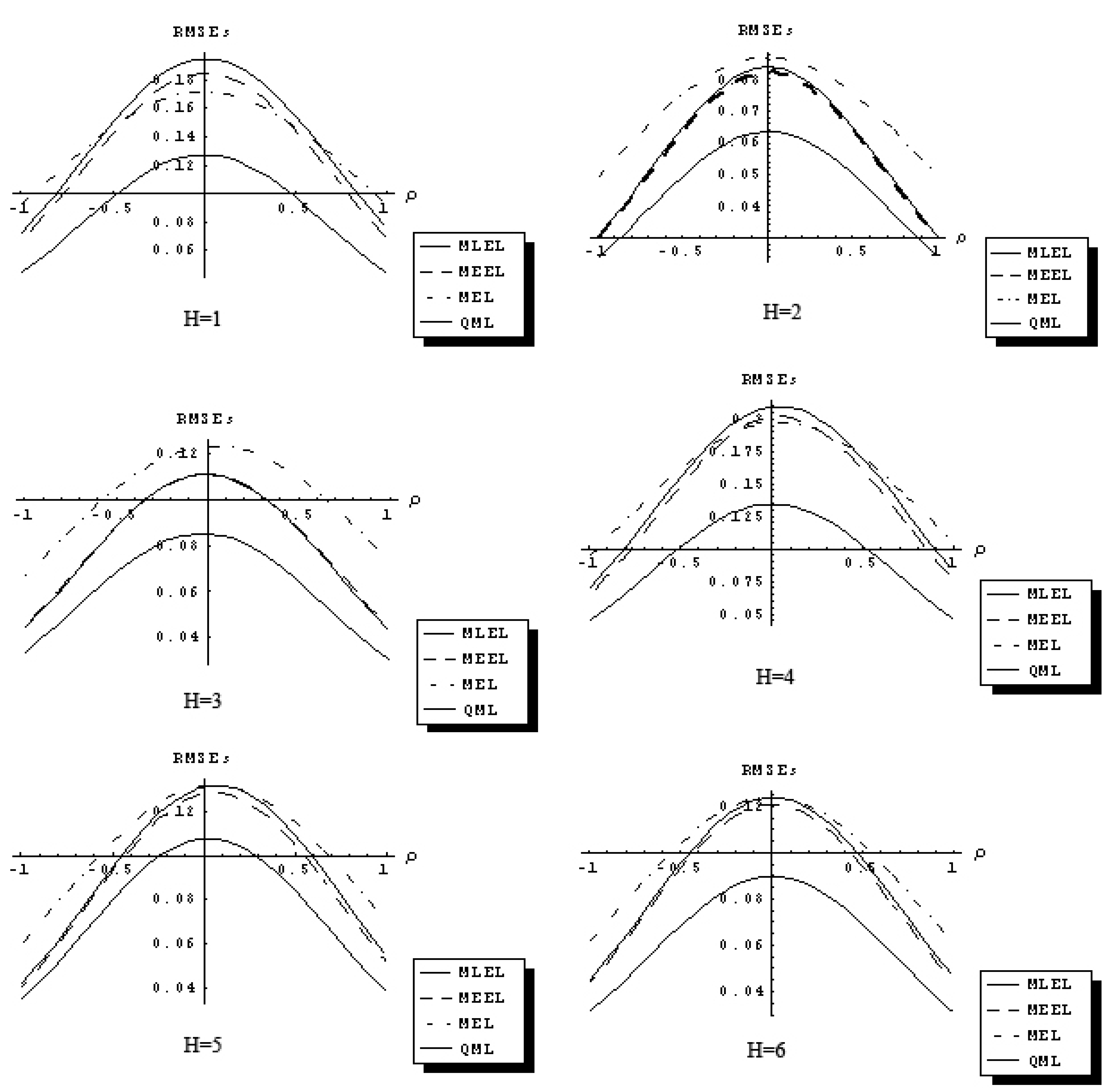
Figure 1.
Response function RMSEs of QML, MEEL, MLEL and MEL of ρ (n = 25 and J = 2).
Figure 1.
Response function RMSEs of QML, MEEL, MLEL and MEL of ρ (n = 25 and J = 2).
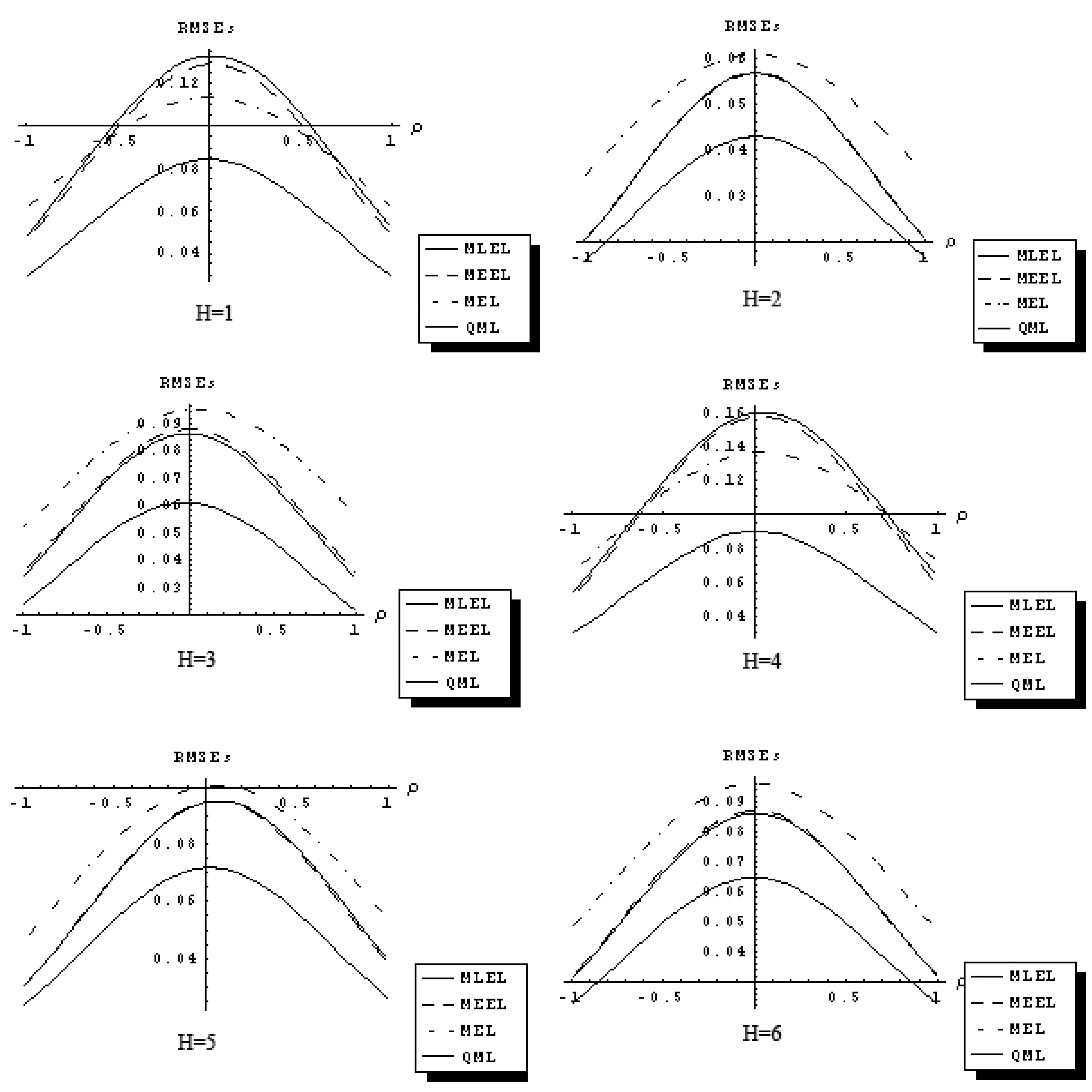
Figure 2.
Response function RMSEs of QML, MEEL, MLEL and MEL of ρ (n = 60 and J = 2).
Figure 2.
Response function RMSEs of QML, MEEL, MLEL and MEL of ρ (n = 60 and J = 2).
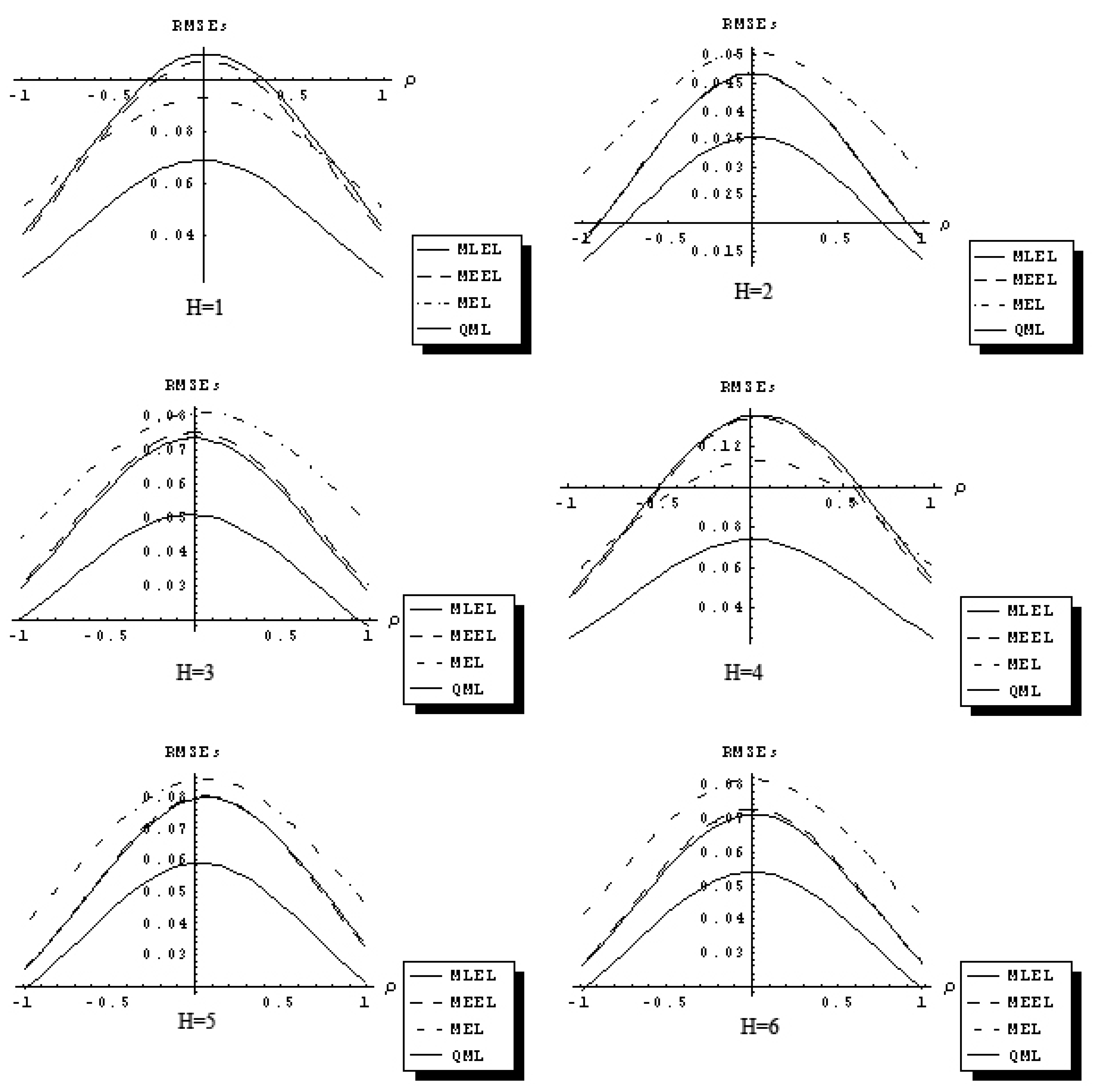
The RMSEs are related to the spatial autocorrelation parameter, ρ, in a concave fashion. The difference in the RMSEs between QML and IT estimators increases as ρ approaches zero, and it decreases as ρ approaches ±1. The QML estimator outperforms the IT estimators for all distributional assumptions considered and for J = 2, 6, 10. The response functions for the three IT estimators considered are related to the ρ in similar fashion and have comparable magnitude. As sample size increases, differences between the response functions of QML and IT estimators declines.
The results of the Monte Carlo study suggest that in certain sampling situations information theoretic estimators of the first-order spatial autoregressive model have superior sampling properties and outperform traditional OLS, 2SLS and GMM estimators with the exception of quasi-maximum likelihood estimator.
Figure 3.
Response function RMSEs of QML, MEEL, MLEL and MEL of ρ (n = 90 and J = 2).
Figure 3.
Response function RMSEs of QML, MEEL, MLEL and MEL of ρ (n = 90 and J = 2).

