Moving Frames of Reference, Relativity and Invariance in Transfer Entropy and Information Dynamics

Abstract

We present a new interpretation of a local framework for information dynamics, including the transfer entropy, by defining a moving frame of reference for the observer of dynamics in lattice systems. This formulation is inspired by the idea of investigating “relativistic” effects on observing the dynamics of information - in particular, we investigate a Galilean transformation of the lattice system data. In applying this interpretation to elementary cellular automata, we demonstrate that using a moving frame of reference certainly alters the observed spatiotemporal measurements of information dynamics, yet still returns meaningful results in this context. We find that, as expected, an observer will report coherent spatiotemporal structures that are moving in their frame as information transfer, and structures that are stationary in their frame as information storage. Crucially, the extent to which the shifted frame of reference alters the results depends on whether the shift of frame retains, adds or removes relevant information regarding the source-destination interaction.

1. Introduction

Einstein’s theory of relativity postulates that the laws of physics are the same for observers in all moving frames of reference (no frame is preferred) and that the speed of light is the same in all frames [1]. These postulates can be used to quantitatively describe the differences in measurements of the same events made by observers in different frames of reference.

Information-theoretic measures are always computed with reference to some observer. They are highly dependent on how the observer measures the data, the subtleties of how an observer asks a question of the data, how the observer attempts to interpret information from the data, and what the observer already knows [2,3]. We aim to take inspiration from the theory of relativity to explore the effect of a moving observer on information-theoretic measures here. To make such an investigation however, we need not only an observer for the information measures but specifically:

(1)

a space-time interpretation for the relevant variables in the system; and

(2)

some frame of reference for the observer, which can be moving in space-time in the system while the measures are computed.

A candidate for such investigations is a recently introduced framework for information dynamics [4,5,6,7,8], which measures information storage, transfer and modification at each local point in a spatiotemporal system. This framework has had success in various domains, particularly in application to cellular automata (CAs), a simple but theoretically important class of discrete dynamical system that is set on a regular space-time lattice. In application to CAs, the framework has provided quantitative evidence for long-held conjectures that the moving coherent structures known as particles are the dominant information transfer entities and that collisions between them are information modification events. In considering the dynamics of information, the framework examines the state updates of each variable in the system with respect to the past state of that variable. For example, in examining the information transfer into a destination variable using the transfer entropy [9], we consider how much information was contributed from some source, in the context of the past state of that destination. This past state can be seen as akin to a stationary frame of reference for the measurement. As such, we have the possibility to use this framework to explore “relativistic” effects on information; i.e., as applied to a spatiotemporal system such as a CA, with a spatiotemporally moving frame of reference. We begin our paper by introducing CAs in Section 2, basic information-theoretic quantities in Section 3, and the measures for information dynamics in Section 4.

Our primary concern in this paper then lies in exploring a new interpretation of this framework for information dynamics by defining and incorporating a moving frame of reference for the observer (Section 5). The type of relativity presented for application to these lattice systems is akin to an ether relativity, where there is a preferred stationary frame in which information transfer is limited by the speed of light. (We note the existence of a discretized special relativity for certain CAs by Smith [10]. For special relativity to be applicable, the CA laws must obey the same rules in all frames of reference. Smith notes the difficulty to find any non-trivial CA rules that meet this requirement, and indeed uses only a simple diffusion process as an example. While in principle we could apply our measures within moving frames of reference in that particular discretization, and intend to do so in future work, we examine only an ether-type of relativity in this study, as this is more naturally applicable to lattice systems.) We also mathematically investigate the shift of frame to demonstrate the invariance of certain information properties. That is, while the total information required to predict a given variable’s value remains the same, shifting the frame of reference redistributes that information amongst the measurements of information storage and transfer by the observer. The nature of that redistribution will depend on whether the shift of frame retains, adds or removes relevant information regarding the source-destination interactions.

We perform experiments on elementary cellular automata (ECAs) using the new perspective on information dynamics with shifted frames of reference in Section 6, comparing the results to those found in the stationary frame. We find that, as expected, the use of a moving frame of reference has a dramatic effect on the measurements of information storage and transfer, though the results are well-interpretable in the context of the shifted frame. In particular, particles only appear as information transfer in frames in which they are moving, otherwise they appear as information storage.

2. Dynamics of Computation in Cellular Automata

Cellular automata (CAs) have been a particular focus for experimentation with the framework for the information dynamics measures that we use here. This is because CAs have been used to model a wide variety of real-world phenomena (see [11]), and have attracted much discussion regarding the nature of computation in their dynamics.

CAs are discrete dynamical systems consisting of an array of cells that each synchronously update their state as a function of the states of a fixed number of spatially neighboring cells using a uniform rule. We focus on Elementary CAs, or ECAs, a simple variety of 1D CAs using binary states, deterministic rules and one neighbor on either side (i.e., cell range $r=1$). An example evolution of an ECA may be seen in Figure 1(a). For more complete definitions, including that of the Wolfram rule number convention for describing update rules (used here), see [12].

Studies of information dynamics in CAs have focused on their emergent structure: particles, gliders, blinkers and domains. A domain is a set of background configurations in a CA, any of which will update to another configuration in the set in the absence of any disturbance. Domains are formally defined by computational mechanics as spatial process languages in the CA [13]. Particles are considered to be dynamic elements of coherent spatiotemporal structure, as disturbances or in contrast to the background domain. Gliders are regular particles, and blinkers are stationary gliders. Formally, particles are defined by computational mechanics as a boundary between two domains [13]; as such, they can be referred to as domain walls, though this term is usually reserved for irregular particles. Several techniques exist to filter particles from background domains (e.g., [5,6,7,13,14,15,16,17,18,19,20]). As a visual example, see Figure 1(a) and Figure 1(b) – the horizontally moving gliders in Figure 1(a) are filtered using negative values of the measure in Figure 1(b) (which will be introduced in Section 4.1), while the domains (in the background) and the blinkers (the stationary large triangular structures) in Figure 1(a) are filtered using positive values of the measure in Figure 1(b).

These emergent structures have been quite important to studies of computation in CAs, for example in the design or identification of universal computation in CAs (see [11]), and in the analyses of the dynamics of intrinsic or other specific computation ([13,21,22]). This is because these studies typically discuss the computation in terms of the three primitive functions of computation and their apparent analogues in CA dynamics [11,21]:

• blinkers as the basis of information storage, since they periodically repeat at a fixed location;
• particles as the basis of information transfer, since they communicate information about the dynamics of one spatial part of the CA to another part; and
• collisions between these structures as information modification, since collision events combine and modify the local dynamical structures.

Previous to recent work however [4,5,6,7] (as discussed in Section 4), these analogies remained conjecture only.

Figure 1. Measures of information dynamics applied to ECA Rule 54 with a stationary frame of reference (all units in (b)–(d) are in bits). Time increases down the page for all plots. (a) Raw CA; (b) Local active information storage $a(i,n,k=16)$; (c) Local apparent transfer entropy $t(i,j=-1,n,k=16)$; (d) Local complete transfer entropy $t^c(i,j=-1,n,k=16)$.

Figure 1. Measures of information dynamics applied to ECA Rule 54 with a stationary frame of reference (all units in (b)–(d) are in bits). Time increases down the page for all plots. (a) Raw CA; (b) Local active information storage $a(i,n,k=16)$; (c) Local apparent transfer entropy $t(i,j=-1,n,k=16)$; (d) Local complete transfer entropy $t^c(i,j=-1,n,k=16)$.

3. Information-theoretic Quantities

To quantify these dynamic functions of computation, we look to information theory (e.g., see [2,3]) which has proven to be a useful framework for the design and analysis of complex self-organized systems, e.g., [23,24,25,26,27]. John: choose which other of your articles you might want to cite here In this section, we give a brief overview of the fundamental quantities which will be built on in the following sections.

The Shannon entropy represents the uncertainty associated with any measurement x of a random variable X (logarithms are in base 2, giving units in bits): $H\left(X\right)=-{\sum }_{x}p\left(x\right)logp\left(x\right)$. The joint entropy of two random variables X and Y is a generalization to quantify the uncertainty of their joint distribution: $H(X,Y)=-{\sum }_{x,y}p(x,y)logp(x,y)$. The conditional entropy of X given Y is the average uncertainty that remains about x when y is known: $H\left(X\right|Y)=-{\sum }_{x,y}p(x,y)logp\left(x\right|y)$. The mutual information between X and Y measures the average reduction in uncertainty about x that results from learning the value of y, or vice versa: $I(X;Y)=H\left(X\right)-H\left(X\right|Y)$. The conditional mutual information between X and Y given Z is the mutual information between X and Y when Z is known: $I(X;Y|Z)=H(X\left|Z\right)-H\left(X\right|Y,Z)$.

Moving to dynamic measures of information in time-series processes X, the entropy rate is the limiting value of the average entropy of the next realizations $x_{n+1}$ of X conditioned on the realizations $x_n^{\left(k\right)}=\left\{x_{n-k+1},\dots ,x_{n-1},x_n\right\}$ of the previous k values $X^{\left(k\right)}$ of X (up to and including time step n):

$$\begin{array}{c}\hfill H_{\mu X}=\underset{k\to \infty }{lim}H\left[X|X^{\left(k\right)}\right]=\underset{k\to \infty }{lim}{H}_{\mu X}\left(k\right)\end{array}$$

(1)

Finally, the effective measure complexity [28] or excess entropy [23] quantifies the total amount of structure or memory in a system, and is computed in terms of the slowness of the approach of the entropy rate estimates to their limiting value (see [23]). For our purposes, it is best formulated as the mutual information between the semi-infinite past and semi-infinite future of the process:

$$\begin{array}{c}\hfill E_X=\underset{k\to \infty }{lim}I\left[X^{\left(k\right)};X^{\left(k^{+}\right)}\right]\end{array}$$

(2)

where $X^{\left(k^{+}\right)}$ refers to the next k states with realizations $x^{\left(k^{+}\right)}=\left\{x_{n+1},x_{n+2},\dots ,x_{n+k}\right\}$. This interpretation is known as the predictive information [29], as it highlights that the excess entropy captures the information in a system’s past that can also be found in its future.

4. Framework for Information Dynamics

A local framework for information dynamics has recently been introduced in [4,5,6,7,8]. This framework examines the information composition of the next value $x_{n+1}$ of a destination variable, in terms of how much of that information came from the past state of that variable (information storage), how much came from respective source variables (information transfer), and how those information sources were combined (information modification). The measures of the framework provide information profiles quantifying each element of computation at each spatiotemporal point in a complex system.

In this section, we describe the information storage and transfer components of the framework (the information modification component is not studied here; it may be seen in [6]). We also review example profiles of these information dynamics in ECA rule 54 (see raw states in Figure 1(a)). ECA rule 54 is considered a class IV complex rule, contains simple glider structures and collisions, and is therefore quite useful in illustrating the concepts around information dynamics.

4.1. Information Storage

We define information storage as the amount of information from the past of a process that is relevant to or will be used at some point in its future. The statistical complexity [30] measures the amount of information in the past of a process that is relevant to the prediction of its future states. It is known that the statistical complexity $C_{\mu X}$ provides an upper bound to the excess entropy [31]; i.e., $E_X\le C_{\mu X}$. This can be interpreted in that the statistical complexity measures all information stored by the system that may be used in the future, whereas the excess entropy only measures the information that is used by the system at some point in the future. Of course, this means that the excess entropy measures information storage that will possibly but not necessarily be used at the next time step $n+1$. When focusing on the dynamics of information processing, we are particularly interested in how much of the stored information is actually in use at the next time step, so as to be examined in conjunction with information transfer.

As such, the active information storage $A_X$ was introduced [7] to explicitly measure how much of the information from the past of the process is observed to be in use in computing its next state. The active information storage is the average mutual information between realizations $x_n^{\left(k\right)}$ of the past state $X^{\left(k\right)}$ (as $k\to \infty$) and the corresponding realizations $x_{n+1}$ of the next value $X^{\prime }$ of a given time series X:

$$\begin{array}{c}\hfill A_X=\underset{k\to \infty }{lim}{A}_X\left(k\right)\end{array}$$

(3)

$$\begin{array}{c}\hfill A_X\left(k\right)=I\left[X^{\left(k\right)};X^{\prime }\right]\end{array}$$

(4)

We note that the limit $k\to \infty$ is required in general, unless the next value $x_{n+1}$ is conditionally independent of the far past values $x_{n-k}^{\left(\infty \right)}$ given $x_n^{\left(k\right)}$.

We can then extract the local active information storage $a_X(n+1)$ [7] as the amount of information storage attributed to the specific configuration or realization $(x_n^{\left(k\right)},x_{n+1})$ at time step $n+1$; i.e., the amount of information storage in use by the process at the particular time-step $n+1$: (Descriptions of the manner in which local information-theoretical measures are obtained from averaged measures may be found in [5,31].)

$$\begin{array}{cc}\hfill A_X& ={〈a_X(n+1)〉}_n\hfill \end{array}$$

(5)

$$\begin{array}{cc}\hfill a_X(n+1)& =\underset{k\to \infty }{lim}{a}_X(n+1,k)\hfill \end{array}$$

(6)

$$\begin{array}{cc}\hfill A_X\left(k\right)& ={〈a_X(n+1,k)〉}_n\hfill \end{array}$$

(7)

$$\begin{array}{cc}\hfill a_X(n+1,k)& ={log}_2\frac{p(x_n^{\left(k\right)},x_{n+1})}{p(x_n^{\left(k\right)})p(x_{n+1})}\hfill \end{array}$$

(8)

$$\begin{array}{cc}& =i(x_n^{\left(k\right)};x_{n+1})\hfill \end{array}$$

(9)

By convention, we use lower case labels for the local values of information-theoretic quantities. Note that $A_X\left(k\right)$ and $a(i,n+1,k)$ represent finite k estimates.

Where the process of interest exists for cells on a lattice structure, we include the index i to identify the variable of interest. This gives the following notation for local active information storage $a(i,n+1)$ in a spatiotemporal system:

$$\begin{array}{cc}\hfill a(i,n+1)& =\underset{k\to \infty }{lim}a(i,n+1,k)\hfill \end{array}$$

(10)

$$\begin{array}{cc}\hfill a(i,n+1,k)& ={log}_2\frac{p(x_{i,n}^{\left(k\right)},x_{i,n+1})}{p(x_{i,n}^{\left(k\right)})p(x_{i,n+1})}\hfill \end{array}$$

(11)

We note that the local active information storage is defined for every spatiotemporal point $(i,n)$ in the lattice system. We have $A(i,k)={〈a(i,n,k)〉}_n$ as the average for variable i. For stationary systems of homogeneous variables where the probability distribution functions are estimated over all variables, it is appropriate to average over all variables also, giving:

$$\begin{array}{c}\hfill A\left(k\right)={〈a(i,n,k)〉}_{i,n}\end{array}$$

(12)

Figure 2(a) shows the local active information as this mutual information between the destination cell and its past history. Importantly, $a(i,n,k)$ may be positive or negative, meaning the past history of the cell can either positively inform us or actually misinform us about its next state. An observer is misinformed where, conditioned on the past history, the observed outcome was relatively unlikely as compared with the unconditioned probability of that outcome (i.e., $p(x_{n+1}|x_n^{\left(k\right)})<p(x_{n+1})$). In deterministic systems (e.g., CAs), negative local active information storage means that there must be strong information transfer from other causal sources.

Figure 2. Local information dynamics for a lattice system with speed of light $c=1$ unit per time step: (a) (left) with stationary frame of reference ($f=0$); (b) (right) with moving frame of reference $f=1$ (i.e., at one cell to the right per unit time step). Red double-headed arrow represents active information storage $a(i,n+1,f)$ from the frame of reference; the blue single-headed arrow represent transfer entropy $t(i,j,n+1,f)$ from each source orthogonal to the frame of reference. Note that the frame of reference in the figures is the path of the moving observer through space-time.

Figure 2. Local information dynamics for a lattice system with speed of light $c=1$ unit per time step: (a) (left) with stationary frame of reference ($f=0$); (b) (right) with moving frame of reference $f=1$ (i.e., at one cell to the right per unit time step). Red double-headed arrow represents active information storage $a(i,n+1,f)$ from the frame of reference; the blue single-headed arrow represent transfer entropy $t(i,j,n+1,f)$ from each source orthogonal to the frame of reference. Note that the frame of reference in the figures is the path of the moving observer through space-time.

As reported in [7], and shown in the sample application to rule 54 in Figure 1(b), when applied to CAs the local active information storage identifies strong positive values in the domain and in blinkers (vertical gliders). For each of these entities, the next state is effectively predictable from the destination’s past. This was the first direct quantitative evidence that blinkers and domains were the dominant information storage entities in CAs. Interestingly for rule 54, the amount of predictability from the past (i.e., the active information storage) is roughly the same for both the blinkers and the background domain (see further discussion in [7]). Furthermore, negative values are typically measured at (the leading edge of) traveling gliders, because the past of the destination (being in the regular domain) would predict domain continuation, which is misinformative when the glider is encountered.

4.2. Information Transfer

Information transfer is defined as the amount of information that a source provides about a destination’s next state that was not contained in the destination’s past. This definition pertains to Schreiber’s transfer entropy measure [9] (which we will call the apparent transfer entropy, as discussed later). The transfer entropy captures the average mutual information from realizations $y_n^{\left(l\right)}$ of the state $Y^{\left(l\right)}$ of a source Y to the corresponding realizations $x_{n+1}$ of the next value $X^{\prime }$ of the destination X, conditioned on realizations $x_n^{\left(k\right)}$ of the previous state $X^{\left(k\right)}$:

$$T_{Y\to X}(k,l)=I\left[Y^{\left(l\right)};X^{\prime }\mid X^{\left(k\right)}\right]$$

(13)

Schreiber emphasized that, unlike the (unconditioned) time-differenced mutual information, the transfer entropy was a properly directed, dynamic measure of information transfer rather than shared information.

In general, one should take the limit as $k\to \infty$ in order to properly represent the previous state $X^{\left(k\right)}$ as relevant to the relationship between the next value $X^{\prime }$ and the source Y [5]. Note that k can be limited here where the next value $x_{n+1}$ is conditionally independent of the far past values $x_{n-k}^{\left(\infty \right)}$ given $(x_n^{\left(k\right)},y_n)$. One than then interpret the transfer entropy as properly representing information transfer [5,32]. Empirically of course one is restricted to finite-k estimates $T_{Y\to X}(k,l)$. Furthermore, where only the previous value $y_n$ of Y is a direct causal contributor to $x_{n+1}$, it is appropriate to use $l=1$ [5,32]. So for our purposes, we write:

$$\begin{array}{c}\hfill T_{Y\to X}=\underset{k\to \infty }{lim}{T}_{Y\to X}\left(k\right)\end{array}$$

(14)

$$\begin{array}{c}\hfill T_{Y\to X}\left(k\right)=I\left[Y;X^{\prime }\mid X^{\left(k\right)}\right]\end{array}$$

(15)

We can then extract the local transfer entropy $t_{Y\to X}(n+1)$ [5] as the amount of information transfer attributed to the specific configuration or realization $(x_{n+1},x_n^{\left(k\right)},y_n)$ at time step $n+1$; i.e., the amount of information transfered from Y to X at time step $n+1$:

$$\begin{array}{cc}\hfill T_{Y\to X}& =〈t_{Y\to X}(n+1)〉\hfill \end{array}$$

(16)

$$\begin{array}{cc}\hfill t_{Y\to X}(n+1)& =\underset{k\to \infty }{lim}{t}_{Y\to X}(n+1,k)\hfill \end{array}$$

(17)

$$\begin{array}{cc}\hfill T_{Y\to X}\left(k\right)& =〈t_{Y\to X}(n+1,k)〉\hfill \end{array}$$

(18)

$$\begin{array}{cc}\hfill t_{Y\to X}(n+1,k)& ={log}_2\frac{p(x_{n+1}\mid x_n^{\left(k\right)},y_n)}{p(x_{n+1}\mid x_n^{\left(k\right)})}\hfill \end{array}$$

(19)

$$\begin{array}{cc}& =i(y_n;x_{n+1}\mid x_n^{\left(k\right)})\hfill \end{array}$$

(20)

Again, where the processes Y and X exist on cells on a lattice system, we denote i as the index of the destination variable $X_i$ and $i-j$ as the source variable $X_{i-j}$, such that we consider the local transfer entropy across j cells in:

$$\begin{array}{cc}\hfill t(i,j,n+1)& =\underset{k\to \infty }{lim}t(i,j,n+1,k)\hfill \end{array}$$

(21)

$$\begin{array}{cc}\hfill t(i,j,n+1,k)& =log\frac{p(x_{i,n+1}|x_{i,n}^{\left(k\right)},x_{i-j,n})}{p(x_{i,n+1}|x_{i,n}^{\left(k\right)})}\hfill \end{array}$$

(22)

The local transfer entropy is defined for every channel j for the given destination i, but for proper interpretation as information transfer j is constrained among causal information contributors to the destination [32] (i.e., within the past light cone [33]). For CAs for example we have $\left|j\right|\le r$, being $\left|j\right|\le 1$ for ECAs as shown in Figure 2(a).

We have $T(i,j,k)={〈t(i,j,n,k)〉}_n$ as the average transfer from variable $i-j$ to variable i. For systems of homogeneous variables where the probability distribution functions for transfer across j cells are estimated over all variables, it is appropriate to average over all variables also, giving:

$$\begin{array}{c}\hfill T(j,k)={〈t(i,j,n,k)〉}_{i,n}\end{array}$$

(23)

Importantly, the information conditioned on by the transfer entropy (i.e., that contained in the destination’s past about its next state) is that provided by the local active information storage. (Note however that a conditional mutual information may be either larger or smaller than the corresponding unconditioned mutual information [3]; the conditioning removes information redundantly held by the source and the conditioned variable, but also includes synergistic information that can only be decoded with knowledge of both the source and conditioned variable [34].)

Also, the local transfer entropy may also be positive or negative. As reported in [5], when applied to CAs it is typically strongly positive when measured at a glider in the same direction j as the macroscopic motion of the glider (see the sample application to rule 54 in Figure 1(c)). Negative values imply that the source misinforms an observer about the next state of the destination in the context of the destination’s past. Negative values are typically only found at gliders for measurements in the orthogonal direction to macroscopic glider motion (see the right moving gliders in Figure 1(c)); at these points, the source (still part of the domain) would suggest that the domain pattern in the destination’s past would continue, which is misinformative. Small positive non-zero values are also often measured in the domain and in the orthogonal direction to glider motion (see Figure 1(c)). These correctly indicate non-trivial information transfer in these regions (e.g., indicating the absence of a glider), though they are dominated by the positive transfer in the direction of glider motion. These results for local transfer entropy provided the first quantitative evidence for the long-held conjecture that particles are the information transfer agents in CAs.

We note that the transfer entropy can also be conditioned on other possible causal contributors Z in order to account for their effects on the destination. We introduced the conditional transfer entropy for this purpose [5,6]:

$$\begin{array}{cc}\hfill T_{Y\to X\mid Z}& =\underset{k\to \infty }{lim}{T}_{Y\to X\mid Z}\left(k\right)\hfill \end{array}$$

(24)

$$\begin{array}{cc}\hfill T_{Y\to X\mid Z}\left(k\right)& =I\left[Y;X^{\prime }\mid X^{\left(k\right)},Z\right]\hfill \end{array}$$

(25)

$$\begin{array}{cc}\hfill T_{Y\to X\mid Z}\left(k\right)& =〈t_{Y\to X\mid Z}(n+1,k)〉\hfill \end{array}$$

(26)

$$\begin{array}{cc}\hfill t_{Y\to X\mid Z}(n+1,k)& ={log}_2\frac{p(x_{n+1}\mid x_n^{\left(k\right)},y_n,z_n)}{p(x_{n+1}\mid x_n^{\left(k\right)},z_n)}\hfill \end{array}$$

(27)

$$\begin{array}{cc}& =i(y_n;x_{n+1}\mid x_n^{\left(k\right)},z_n)\hfill \end{array}$$

(28)

This extra conditioning can exclude the (redundant) influence of a common drive Z from being attributed to Y, and can also include the synergistic contribution when the source Y acts in conjunction with another source Z (e.g., where X is the outcome of an XOR operation on Y and Z).

We specifically refer to the conditional transfer entropy as the complete transfer entropy (with notation $T_{Y\to X}^c\left(k\right)$ and $t_{Y\to X}^c(n+1,k)$ for example) when it conditions on all other causal sources Z to the destination X [5]. For CAs, this means conditioning on the only other causal contributor to the destination. For example, for the $j=1$ channel, we can write

$$\begin{array}{cc}\hfill t^c(i,j=1,n+1)& =\underset{k\to \infty }{lim}{t}^c(i,j=1,n+1,k)\hfill \end{array}$$

(29)

$$\begin{array}{cc}\hfill t^c(i,j=1,n+1,k)& =log\frac{p(x_{i,n+1}|x_{i,n}^{\left(k\right)},x_{i-1,n},x_{i+1,n})}{p(x_{i,n+1}|x_{i,n}^{\left(k\right)},x_{i+1,n})}\hfill \end{array}$$

(30)

with $T^c(j,k)$ for the spatiotemporal average in homogeneous, stationary systems. To differentiate the conditional and complete transfer entropies from the original measure, we often refer to $T_{Y\to X}$ simply as the apparent transfer entropy [5]—this nomenclature conveys that the result is the information transfer that is apparent without accounting for other sources.

In application to CAs, we note that the results for $t^c(i,j,n+1,k)$ are largely the same as for $t(i,j,n+1,k)$ (e.g., compare Figure 1(d) with Figure 1(c) for rule 54), with some subtle differences. These results are discussed in detail in [5]. First, in deterministic systems such as CAs, $t^c(i,j,n+1,k)$ cannot be negative since by accounting for all causal sources (and without noise) there is no way that our source can misinform us about the next state of the destination. Also, the strong transfer measured in gliders moving in the macroscopic direction of the measured channel j is slightly stronger with $t^c(i,j,n+1,k)$. This is because, by accounting for the other causal source, we can be sure that there is no other incoming glider to disturb this one, and thus attribute more influence to the source of the ongoing glider here. Other scenarios regarding synergistic interactions in other rules are discussed in [5].

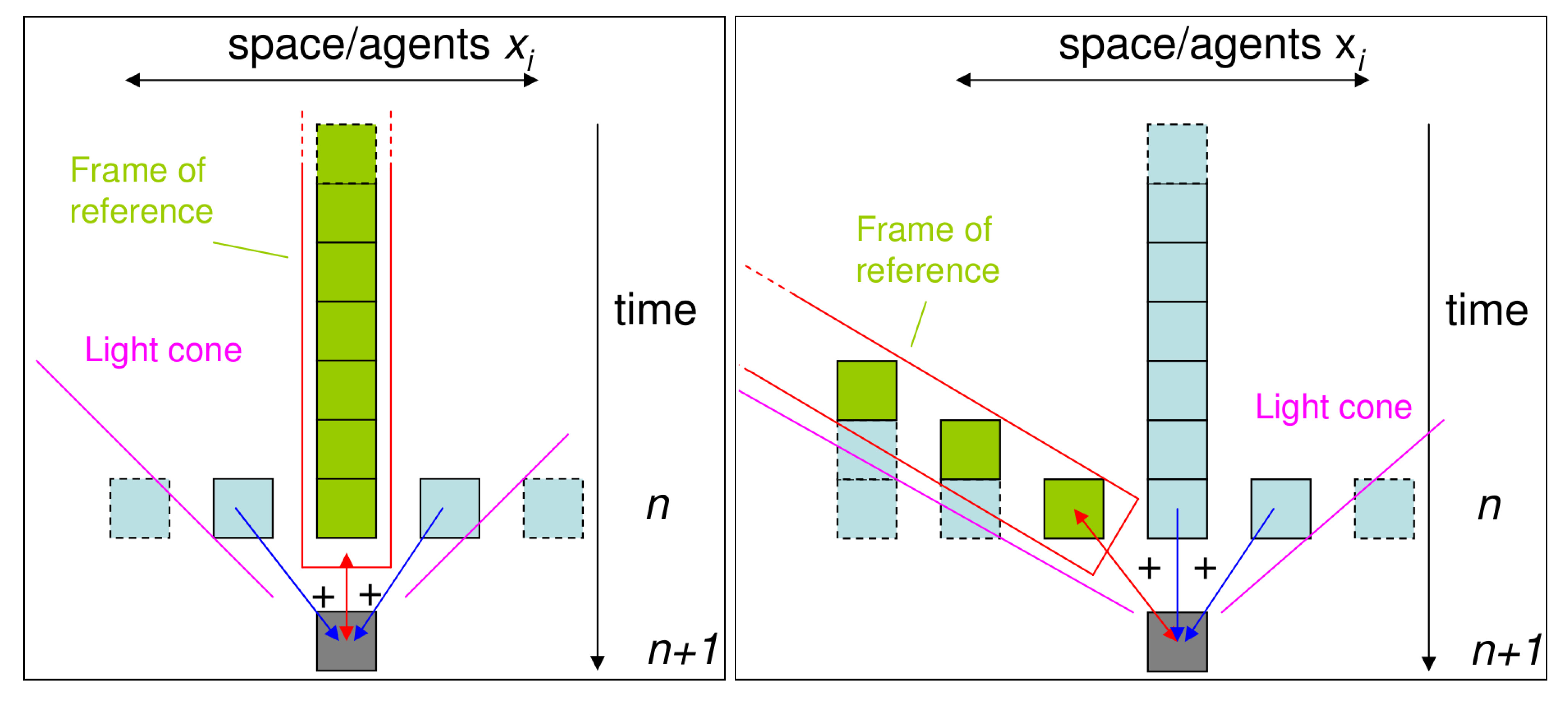
5. Information Dynamics for a Moving Observer

In this section, we consider how these measures of information dynamics would change for a moving observer. First, we consider the meaning of the past state $x_n^{\left(k\right)}$ in these measures, and how it can be interpreted as a frame of reference. We then provide a formulation to interpret these measures for an observer with a moving frame of reference. We consider what aspects of the dynamics would remain invariant, and finally consider what differences we may expect to see from measures of information dynamics by moving observers.

5.1. Meaning of the Use of the Past State

Realizations $x_n^{\left(k\right)}$ of the past state $X^{\left(k\right)}$ of the destination variable X play a very important role in the measures of information dynamics presented above. We see that the active information storage directly considers the amount of information contained in $x_n^{\left(k\right)}$ about the next value $x_{n+1}$ of X, while the transfer entropy considers how much information the source variable adds to this next value conditioned on $x_n^{\left(k\right)}$.

The role of the past state $x_n^{\left(k\right)}$ can be understood from three complementary perspectives here:

(1)

To separate information storage and transfer. As described above, we know that $x_n^{\left(k\right)}$ provides information storage for use in computation of the next value $x_{n+1}$. The conditioning on the past state in the transfer entropy ensures that none of that information storage is counted as information transfer (where the source and past hold some information redundantly) [5,6].

(2)

To capture the state transition of the destination variable. We note that Schreiber’s original description of the transfer entropy [9] can be rephrased as the information provided by the source about the state transition in the destination. That $x_n^{\left(k\right)}\to x_{n+1}$ (or including redundant information $x_n^{\left(k\right)}\to x_{n+1}^{\left(k\right)}$) is a state transition is underlined in that the $x_n^{\left(k\right)}$ are embedding vectors [35], which capture the underlying state of the process.

(3)

To examine the information composition of the next value $x_{n+1}$ of the destination in the context of the past state $x_n^{\left(k\right)}$ of the destination. With regard to the transfer entropy, we often describe the conditional mutual information as “conditioning out” the information contained in $x_n^{\left(k\right)}$, but this nomenclature can be slightly misleading. This is because, as pointed out in Section 4.2, a conditional mutual information can be larger or smaller than the corresponding unconditioned form, since the conditioning both removes information redundantly held by the source variable and the conditioned variable (e.g., if the source is a copy of the conditioned variable) and adds information synergistically provided by the source and conditioned variables together (e.g., if the destination is an XOR-operation of these variables). As such, it is perhaps more useful to describe the conditioned variable as providing context to the measure, rather than “conditioning out” information. Here then, we can consider the past state $x_n^{\left(k\right)}$ as providing context to our analysis of the information composition of the next value $x_{n+1}$.

Note that we need $k\to \infty$ to properly capture each perspective here (see discussion in Section 4.1 and Section 4.2 regarding conditions where finite-k is satisfactory).

Importantly, we note that the final perspective of $x_n^{\left(k\right)}$ as providing context to our analysis of the information composition of the computation of the next state can also be viewed as a “frame of reference” for the analysis.

5.2. Information Dynamics with a Moving Frame of Reference

Having established the perspective of $x_n^{\left(k\right)}$ as providing a frame of reference for our analysis, we now examine how the measures of our framework are altered if we consider a moving frame of reference for our observer in lattice systems.

It is relatively straightforward to define a frame of reference for an observer moving at f cells per unit time towards the destination cell $x_{i,n+1}$. Our measures consider the set of k cells backwards in time from $x_{i,n+1}$ at $-f$ cells per time step:

$$\begin{array}{cc}\hfill x_{i-f,n}^{(k,f)}& =\left\{x_{i-(q+1)f,n-q}\right|0\le q<k\}\hfill \end{array}$$

(31)

$$\begin{array}{cc}& =\{x_{i-kf,n-k+1},...,x_{i-2f,n-1},x_{i-f,n}\}\hfill \end{array}$$

(32)

Notice that $x_{i,n}^{\left(k\right)}=x_{i-0,n}^{(k,0)}$ with $f=0$, as it should.

We can then define measures for each of the information dynamics in this new frame of reference f. As shown with the double headed arrow in Figure 2(b), the local active information in this frame becomes the local mutual information between the observer’s frame of reference $x_{i-f,n}^{(k,f)}$ and the next state of the destination cell $x_{i,n+1}$; mathematically this is represented by:

$$\begin{array}{cc}\hfill a(i,n+1,f)& =\underset{k\to \infty }{lim}a(i,n+1,k,f)\hfill \end{array}$$

(33)

$$\begin{array}{cc}\hfill a(i,n+1,k,f)& =log\frac{p(x_{i-f,n}^{(k,f)},x_{i,n+1})}{p(x_{i-f,n}^{(k,f)})p(x_{i,n+1})}\hfill \end{array}$$

(34)

Crucially, $a(i,n+1,k,f)$is still a measure of local information storage for the moving observer: it measures how much information is contained in the past of their frame of reference about the next state that appears in their frame. The observer, as well as the shifted measure itself, is oblivious to the fact that these observations are in fact taken over different variables. Finally, we write $A(k,f)={〈a(i,n+1,k,f)〉}_{i,n}$ as the average of finite-k estimates over all space-time points $(i,n)$ in the lattice, for stationary homogeneous systems.

As shown by directed arrows in Figure 2(b), the local transfer entropy becomes the local conditional mutual information between the source cell $x_{i-j,n}$ and the destination $x_{i,n+1}$, conditioned on the moving frame of reference $x_{i-f,n}^{(k,f)}$:

$$\begin{array}{cc}\hfill t(i,j,n+1,f)& =\underset{k\to \infty }{lim}t(i,j,n+1,k,f)\hfill \end{array}$$

(35)

$$\begin{array}{cc}\hfill t(i,j,n+1,k,f)& =log\frac{p(x_{i,n+1}|x_{i-f,n}^{(k,f)},x_{i-j,n})}{p(x_{i,n+1}|x_{i-f,n}^{(k,f)})}\hfill \end{array}$$

(36)

The set of sensible values to use for j remains those within the light-cone (i.e., those that represent causal information sources to the destination variable); otherwise we only measure correlations rather than information transfer. That said, we also do not consider the transfer entropy for the channel $j=f$ here, since this source is accounted for by the local active information. Of course, we can now also consider $j=0$ for moving frames $f\ne 0$. Writing the local complete transfer entropy $t^c(i,j,n+1,k,f)$ for the moving frame trivially involves adding conditioning on the remaining causal source (that which is not the source $x_{i-j,n}$ itself, nor the source $x_{i-f,n}$ in the frame) to Equation (36).

Again, $t(i,j,n+1,f)$ is still interpretable as a measure of local information transfer for the moving observer: it measures how much information was provided by the source cell about the state transition of the observer’s frame of reference. The observer is oblivious to the fact that the states in its frame of reference are composed of observations taken over different variables.

Also, note that while $t(i,j,n+1,f)$ describes the transfer across j cells in a stationary frame as observed in a frame moving at speed f, we could equally express it as the transfer observed across $j-f$ cells in the frame f.

Finally, we write $T(j,k,f)={〈t(i,j,n+1,k,f)〉}_{i,n}$ as the average of finite-k estimates over all space-time points $(i,n)$ in the lattice, for stationary homogeneous systems.

In the next two subsections, we describe what aspects of the information dynamics remain invariant, and how we can expect the measures to change, with a moving frame of reference.

5.3. Invariance

This formulation suggests the question of why we consider the same set of information sources j in the moving and stationary frames (i.e., those within the light-cone), rather than say a symmetric set of sources around the frame of reference (as per a stationary frame). To examine this, consider the local (single-site) entropy $h(i,n+1)=logp\left(x_{i,n+1}\right)$ as a sum of incrementally conditioned mutual information terms as presented in [6]. For ECAs (a deterministic system), in the stationary frame of reference, this sum is written as:

$$\begin{array}{cc}\hfill h(i,n+1)=& i(x_{i,n}^{\left(k\right)};x_{i,n+1})+i(x_{i-j,n};x_{i,n+1}|x_{i,n}^{\left(k\right)})\hfill \end{array}$$

$$\begin{array}{cc}& +i(x_{i+j,n};x_{i,n+1}|x_{i,n}^{\left(k\right)},x_{i-j,n})\hfill \end{array}$$

(37)

$$\begin{array}{cc}\hfill h(i,n+1)=& a(i,n+1,k)+t(i,j,n+1,k)\hfill \end{array}$$

$$\begin{array}{cc}& +t^c(i,-j,n+1,k)\hfill \end{array}$$

(38)

with either $j=1$ or $j=-1$. Since $h(i,n+1)$ represents the information required to predict the state at site $(i,n+1)$, Equation (37) shows that one can obtain this by considering the information contained in the past of the destination, then the information contributed through channel j that was not in this past, then that contributed through channel $-j$ which was not in this past or the channel j. The first term here is the active information storage, the first local conditional mutual information term here is a transfer entropy, the second is a complete transfer entropy. Considering any sources in addition to or instead of these will only return correlations to the information provided by these entities.

Note that there is no need to take the limit $k\to \infty$ for the correctness of Equation (37) (unless one wishes to properly interpret the terms as information storage and transfer). In fact, the sum of incrementally conditional mutual information terms in Equation (37) is invariant as long as all terms use the same context. We can also consider a moving frame of reference as this context and so construct this sum for a moving frame of reference f. Note that the choice of f determines which values to use for j, so we write an example with $f=1$:

$$\begin{array}{cc}\hfill h(i,n+1)=& a(i,n+1,k,f=1)+t(i,j=0,n+1,k,f=1)\end{array}$$

$$\begin{array}{cc}& +t^c(i,j=-1,n+1,k,f=1)\end{array}$$

(39)

Obviously this is true because the set of causal information contributors is invariant, and we are merely considering the same causal sources but in a different context. Equation (39) demonstrates that prediction of the next state for a given cell in a moving frame of reference depends on the same causal information contributors. Considering the local transfer entropy from sources outside the light cone instead may be insufficient to predict the next state [32].

Choosing the frame of reference here merely sets the context for the information measures, and redistributes the attribution of the invariant amount of information in the next value $x_{i,n+1}$ between the various storage and transfer sources. This could be understood in terms of the different context redistributing the information atoms in a partial information diagram (see [34]) of the sources to the destination.

Note that we examine a type of ether relativity for local information dynamics. That is to say, there is a preferred stationary frame of reference $f=0$ in which the velocity for information is bounded by the speed of light c. The stationary frame of reference is preferred because it is the only frame that has an even distribution of causal information sources on either side, while other frames observe an asymmetric distribution of causal information sources. It is also the only frame of reference that truly represents the information storage in the causal variables. As pointed out in Section 1, we do not consider a type of relativity where the rules of physics (i.e., CA rules) are invariant, remaining observationally symmetric around the frame of reference.

5.4. Hypotheses and Expectations

In general, we expect the measures $a(i,n,k,f)$ and $t(i,j,n,k,f)$ to be different from the corresponding measurements in a stationary frame of reference. Obviously, this is because the frames of reference $x_{i-f,n}^{(k,f)}$ provide in general different contexts for the measurements. As exceptional cases however, the measurements would not change if:

• The two contexts or frames of reference in fact provide the same information redundantly about the next state (and in conjunction with the sources for transfer entropy measurements).
• Neither context provides any relevant information about the next state at all.

Despite such differences to the standard measurements, as described in Section 5.2 the measurements in a moving frame of reference are still interpretable as information storage and transfer for the moving observer, and still provide relevant insights into the dynamics of the system.

In the next section, we will examine spatiotemporal information profiles of CAs, as measured by a moving observer. We hypothesize that in a moving frame of reference f, we shall observe:

• Regular background domains appearing as information storage regardless of movement of the frame of reference, since their spatiotemporal structure renders them predictable in both moving and stationary frames. In this case, both the stationary and moving frames would retain the same information redundantly regarding how their spatiotemporal pattern evolves to give the next value of the destination in the domain;
• Gliders moving at the speed of the frame appearing as information storage in the frame, since the observer will find a large amount of information in their past observations that predict the next state observed. In this case, the shift of frame incorporates different information into the new frame of reference, making that added information appear as information storage;
• Gliders that were stationary in the stationary frame appearing as information transfer in the channel $j=0$ when viewed in moving frames, since the $j=0$ source will add a large amount of information for the observer regarding the next state they observe. In this case, the shift of frame of reference removes relevant information from the new frame of reference, allowing scope for the $j=0$ source to add information about the next observed state.

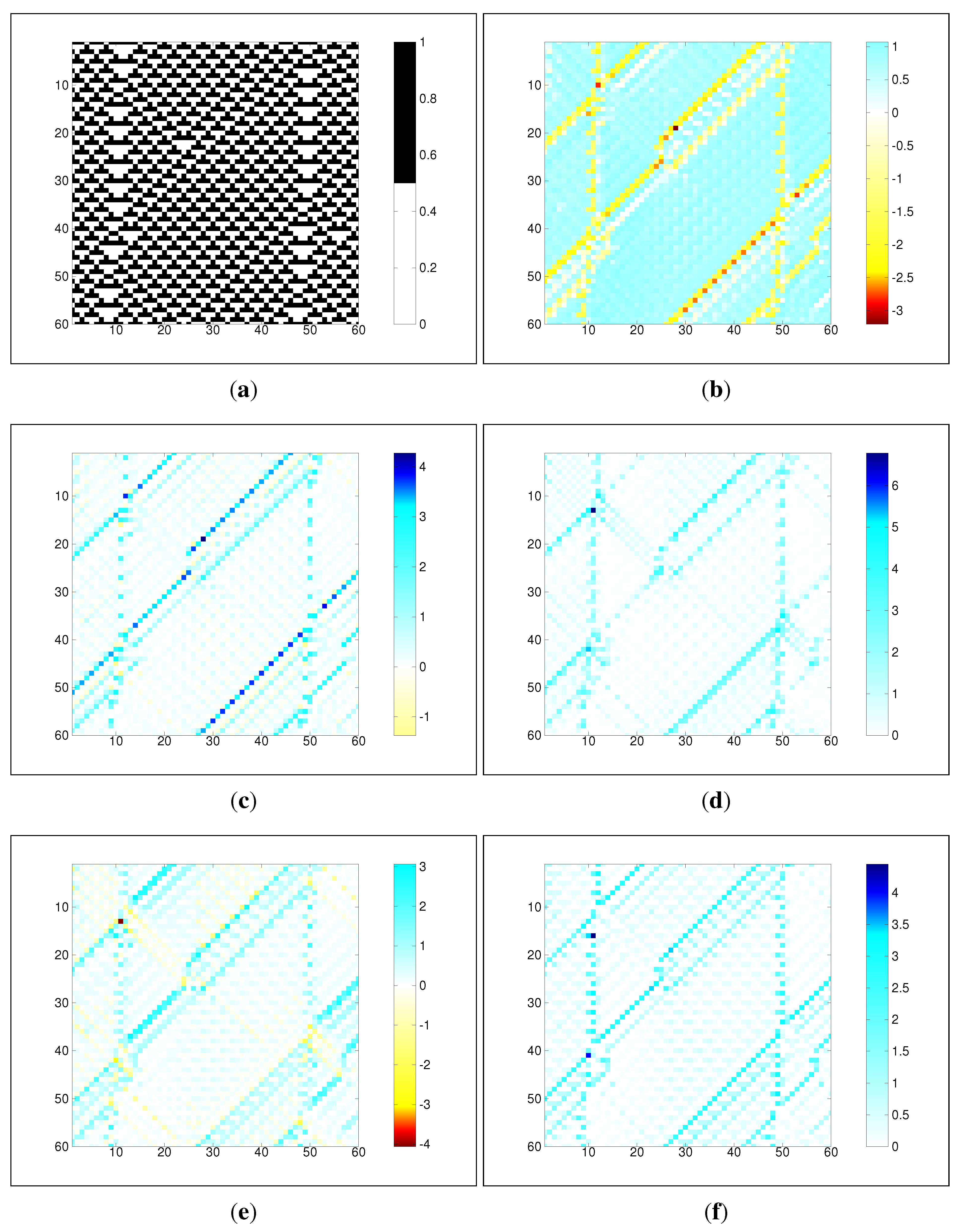
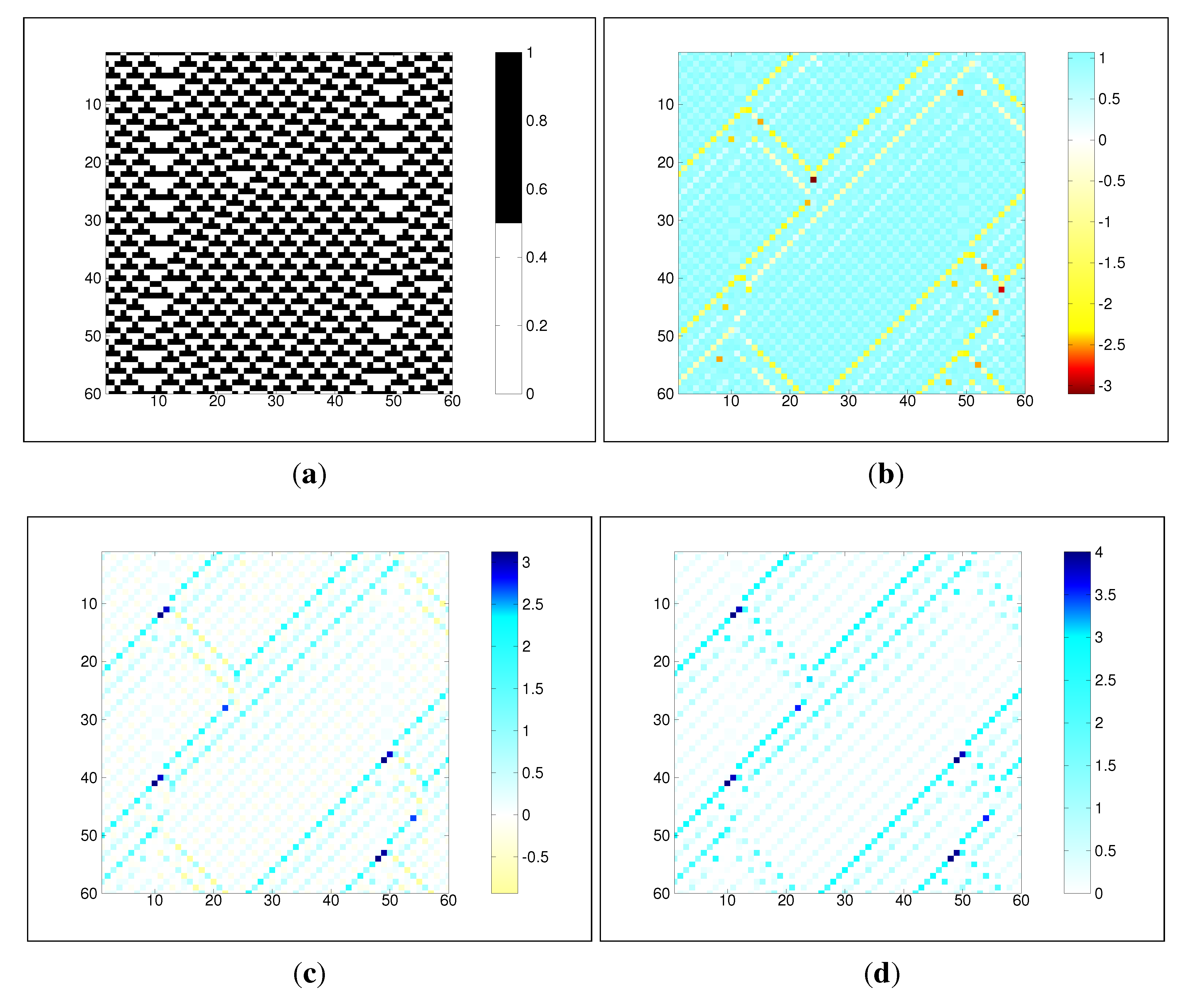
6. Results and Discussion

To investigate the local information dynamics in a moving frame of reference, we study ECA rule 54 here with a frame of reference moving at $f=1$ (i.e., one step to the right per unit time). Our experiments used 10,000 cells initialized in random states, with 600 time steps captured for estimation of the probability distribution functions (similar settings used in introducing the local information dynamics in [5,6,7]). We fixed $k=16$ for our measures (since the periodic background domain for ECA rule 54 has a period of 4, this captures an adequate amount of history to properly separate information storage and transfer as discussed in [5]). We measure the local information dynamics measures in both the stationary frame of reference (Figure 1) and the moving frame of reference $f=1$ (Figure 3). The results were produced using the “Java Information Dynamics Toolkit” [36], and can be reproduced using the Matlab/Octave script movingFrame.m in the demos/octave/CellularAutomata example distributed with this toolkit.

We first observe that the background domain is captured as a strong information storage process irrespective of whether the frame of reference is moving (with $a(i,n,k=16,f=1)$, Figure 3(b)) or stationary (with $a(i,n,k=16,f=0)$, Figure 1(b)). That is to say that the frame of reference is strongly predictive of the next state in the domain, regardless of whether the observer is stationary or moving. This is as expected, because the background domain is not only temporally periodic, but spatiotemporally periodic, and the moving frame provides much redundant information with the stationary frame about the next observed state.

While it is not clear from the local profiles however, the average active information storage is significantly lower for the moving frame than the stationary frame ($A(i,n,k=16,f=1)=0.468$ bits versus $A(i,n,k=16,f=0)=0.721$ bits). At first glance, this seems strange since the background domain is dominated by information storage, and the observer in both frames should be able to adequately detect the periodic domain process. On closer inspection though, we can see that the storage process in the domain is significantly more disturbed by glider incidence in the moving frame, with a larger number and magnitude of negative local values encountered, and more time for the local values to recover to their usual levels in the domain. This suggests that the information in the moving frame is not fully redundant with the stationary frame, which could be explained in that the stationary frame (being centred in the light cone) is better able to retain information about the surrounding dynamics that could influence the next state. The moving frame (moving at the speed of light itself) is not able to contain any information regarding incoming dynamics from neighboring cells. Thus, in the moving frame, more of the (invariant) information in the next observed state is distributed amongst the transfer sources.

As expected also, we note that gliders that are moving at the same speed as the frame of reference $f=1$ are now considered as information storage in that frame. That is, the right moving gliders previously visible as misinformative storage in Figure 1(b) now blend in with the background information storage process in the moving frame in Figure 3(b). As previously discussed, this is because the moving frame brings new information for the observer about these gliders into the frame of reference.

Figure 3(b) also shows that it is only gliders moving in orthogonal directions to the frame $f=1$ (including blinkers, which were formerly considered stationary) that contain negative local active information storage, and are therefore information transfer processes in this frame. Again, this is as expected, since these gliders contribute new information about the observed state in the context of the frame of reference. For gliders that now become moving in the moving frame of reference, this is because the information about those gliders is no longer in the observer’s frame of reference but can now be contributed to the observer by the neighboring sources. To understand these processes in more detail however, we consider the various sources of that transfer via the transfer entropy measurements in Figure 3(c)–Figure 3(f).

First, we focus on the vertical gliders that were stationary in the stationary frame of reference (i.e., the blinkers): we had expected that these entities would be captured as information transfer processes in the $j=0$ (vertical) channel in the $j=1$ moving frame. This expectation is upheld, but the dynamics are more complicated than the foreseen in our hypothesis. Here, we see that the apparent transfer entropy from the $j=0$ source alone does not dominate the dynamics for this vertical glider (Figure 3(c)). Instead, the information transfer required to explain the vertical gliders is generally a combination of both apparent and complete transfer entropy measures, requiring the $j=-1$ source for interpretation as well. The full information may be accounted for by either taking Figure 3(c) plus Figure 3(f) or Figure 3(e) plus Figure 3(d) (as per the two different orders of considering sources to sum the invariant information in Equation (38)). Further, we note that some of the points within the glider are even considered as strong information storage processes - note how there are positive storage points amongst the negative points (skewed by the moving frame) for this glider in Figure 3(b). These vertical gliders are thus observed in this frame of reference to be a complex structure consisting of some information storage, as well as information transfer requiring both other sources for interpretation. This is a perfectly valid result, demonstrating that switching frames of reference does not lead to the simple one-to-one correspondence between individual information dynamics that one may naively expect.

Figure 3. Measures of local information dynamics applied to ECA rule 54, computed in frame of reference $f=1$, i.e., moving 1 cell to the right per unit time (all units in (b)–(f) are in bits). Note that raw states are the same as in Figure 1. (a) Raw CA; (b) Local active information storage $a(i,n,k=16,f=1)$; (c) Local apparent transfer entropy $t(i,j=0,n,k=16,f=1)$; (d) Local complete transfer entropy $t^c(i,j=0,n,k=16,f=1)$; (e) Local apparent transfer entropy $t(i,j=-1,n,k=16,f=1)$; (f) Local complete transfer entropy $t^c(i,j=-1,n,k=16,f=1)$.

Figure 3. Measures of local information dynamics applied to ECA rule 54, computed in frame of reference $f=1$, i.e., moving 1 cell to the right per unit time (all units in (b)–(f) are in bits). Note that raw states are the same as in Figure 1. (a) Raw CA; (b) Local active information storage $a(i,n,k=16,f=1)$; (c) Local apparent transfer entropy $t(i,j=0,n,k=16,f=1)$; (d) Local complete transfer entropy $t^c(i,j=0,n,k=16,f=1)$; (e) Local apparent transfer entropy $t(i,j=-1,n,k=16,f=1)$; (f) Local complete transfer entropy $t^c(i,j=-1,n,k=16,f=1)$.

We note a similar result for the left-moving gliders in the $j=-1$ channel, which are considering moving both in the stationary and $j=1$ frames of reference: here we see that the complete transfer entropy from the $j=0$ source (Figure 3(d)) is required to completely explain some of these gliders. What is interesting is that the (extra) complete transfer entropy from the $j=0$ source orthogonal to the glider is a greater proportion here than for orthogonal sources in the stationary frame (see the complete transfer entropy for the right moving gliders in Figure 1(d)). This suggests that there was less information pertinent to these gliders in the moving frame of reference than there was in the stationary frame. Clearly, a change of frame of reference can lead to complicated interplays between the information dynamics in each frame, with changes in both the magnitude and source attribution of the information.

Finally, note that while one can easily write down the differences between the measures in each frame (e.g., subtracting Equation (11) from Equation (34)), there do not appear to be any clear general principals regarding how the information will be redistributed between storage and transfers for an observer, since this depends on the common information between each frame of reference.

7. Conclusions

In this paper, we have presented a new interpretation of a framework for local information dynamics (including transfer entropy), which incorporates a moving frame of reference for the observer. This interpretation was inspired by the idea of investigating relativistic effects on information dynamics, and indeed contributes some interesting perspectives to this field.

We reported the results from investigations to explore this perspective applied to cellular automata, showing that moving elements of coherent spatiotemporal structure (particles or gliders) are identified as information transfer in frames in which they are moving and as information storage in frames where they are stationary, as expected. Crucially, the extent to which the shifted frame of reference alters the results depends on whether the shift of frame retains, adds or removes relevant information regarding the source-destination interaction. We showed examples illustrating each of these scenarios, and it is important to note that we showed all three to occur at different local points in the same coupled system (i.e., these differences are not mutually exclusive).

Future work may include exploring mathematically formalizing transformation laws between individual information dynamics under shifts of frames of reference, as well as time-reversibility, and the use of different frames of reference as a classification tool.

References

1. Halliday, D.; Resnick, R.; Walker, J. Fundamentals of Physics, 4th ed.; John Wiley & Sons: New York, NY, USA, 1993. [Google Scholar]
2. Cover, T.M.; Thomas, J.A. Elements of Information Theory; John Wiley & Sons: New York, NY, USA, 1991. [Google Scholar]
3. MacKay, D.J. Information Theory, Inference, and Learning Algorithms; Cambridge University Press: Cambridge, UK, 2003. [Google Scholar]
4. Lizier, J.T.; Prokopenko, M.; Zomaya, A.Y. Detecting Non-trivial Computation in Complex Dynamics. In Proceedings of the 9th European Conference on Artificial Life (ECAL 2007), Lisbon, Portugal, 10–14 September 2007; Almeidae Costa, F., Rocha, L.M., Costa, E., Harvey, I., Coutinho, A., Eds.; Springer: Berlin / Heidelberg, 2007; Vol. 4648, Lecture Notes in Computer Science. pp. 895–904. [Google Scholar]
5. Lizier, J.T.; Prokopenko, M.; Zomaya, A.Y. Local information transfer as a spatiotemporal filter for complex systems. Phys. Rev. E 2008, 77, 026110+. [Google Scholar] [CrossRef]
6. Lizier, J.T.; Prokopenko, M.; Zomaya, A.Y. Information modification and particle collisions in distributed computation. Chaos 2010, 20, 037109+. [Google Scholar] [CrossRef] [PubMed]
7. Lizier, J.T.; Prokopenko, M.; Zomaya, A.Y. Local measures of information storage in complex distributed computation. Inform. Sciences 2012, 208, 39–54. [Google Scholar] [CrossRef]
8. Lizier, J.T. The local information dynamics of distributed computation in complex systems; Springer Theses, Springer: Berlin / Heidelberg, Germany, 2013. [Google Scholar]
9. Schreiber, T. Measuring Information Transfer. Phys. Rev. Lett. 2000, 85, 461–464. [Google Scholar] [CrossRef] [PubMed]
10. Smith, M.A. Cellular automata methods in mathematical physics. PhD thesis, Massachusetts Institute of Technology, 1994. [Google Scholar]
11. Mitchell, M. Computation in Cellular Automata: A Selected Review. In Non-Standard Computation; Gramss, T., Bornholdt, S., Gross, M., Mitchell, M., Pellizzari, T., Eds.; VCH Verlagsgesellschaft: Weinheim, Germany, 1998; pp. 95–140. [Google Scholar]
12. Wolfram, S. A New Kind of Science; Wolfram Media: Champaign, IL, USA, 2002. [Google Scholar]
13. Hanson, J.E.; Crutchfield, J.P. The Attractor-Basin Portait of a Cellular Automaton. J. Stat. Phys. 1992, 66, 1415–1462. [Google Scholar] [CrossRef]
14. Grassberger, P. New mechanism for deterministic diffusion. Phys. Rev. A 1983, 28, 3666. [Google Scholar] [CrossRef]
15. Grassberger, P. Long-range effects in an elementary cellular automaton. J. Stat. Phys. 1986, 45, 27–39. [Google Scholar] [CrossRef]
16. Hanson, J.E.; Crutchfield, J.P. Computational mechanics of cellular automata: An example. Physica D 1997, 103, 169–189. [Google Scholar] [CrossRef]
17. Wuensche, A. Classifying cellular automata automatically: Finding gliders, filtering, and relating space-time patterns, attractor basins, and the Z parameter. Complexity 1999, 4, 47–66. [Google Scholar] [CrossRef]
18. Helvik, T.; Lindgren, K.; Nordahl, M.G. Local information in one-dimensional cellular automata. In Proceedings of the International Conference on Cellular Automata for Research and Industry, Amsterdam; Sloot, P.M., Chopard, B., Hoekstra, A.G., Eds.; Springer: Berlin/Heidelberg, Germany, 2004; Vol. 3305, Lecture Notes in Computer Science. pp. 121–130. [Google Scholar]
19. Helvik, T.; Lindgren, K.; Nordahl, M.G. Continuity of Information Transport in Surjective Cellular Automata. Commun. Math. Phys. 2007, 272, 53–74. [Google Scholar] [CrossRef]
20. Shalizi, C.R.; Haslinger, R.; Rouquier, J.B.; Klinkner, K.L.; Moore, C. Automatic filters for the detection of coherent structure in spatiotemporal systems. Phys. Rev. E 2006, 73, 036104. [Google Scholar] [CrossRef]
21. Langton, C.G. Computation at the edge of chaos: phase transitions and emergent computation. Physica D 1990, 42, 12–37. [Google Scholar] [CrossRef]
22. Mitchell, M.; Crutchfield, J.P.; Hraber, P.T. Evolving Cellular Automata to Perform Computations: Mechanisms and Impediments. Physica D 1994, 75, 361–391. [Google Scholar] [CrossRef]
23. Crutchfield, J.P.; Feldman, D.P. Regularities unseen, randomness observed: Levels of entropy convergence. Chaos 2003, 13, 25–54. [Google Scholar] [CrossRef] [PubMed]
24. Prokopenko, M.; Gerasimov, V.; Tanev, I. Evolving Spatiotemporal Coordination in a Modular Robotic System. In Ninth International Conference on the Simulation of Adaptive Behavior (SAB’06); Nolfi, S., Baldassarre, G., Calabretta, R., Hallam, J., Marocco, D., Meyer, J.A., Parisi, D., Eds.; Springer Verlag: Rome, Italy, 2006; Volume 4095, Lecture Notes in Artificial Intelligence; pp. 548–559. [Google Scholar]
25. Prokopenko, M.; Lizier, J.T.; Obst, O.; Wang, X.R. Relating Fisher information to order parameters. Phys. Rev. E 2011, 84, 041116+. [Google Scholar] [CrossRef]
26. Mahoney, J.R.; Ellison, C.J.; James, R.G.; Crutchfield, J.P. How hidden are hidden processes? A primer on crypticity and entropy convergence. Chaos 2011, 21, 037112+. [Google Scholar] [CrossRef] [PubMed]
27. Crutchfield, J.P.; Ellison, C.J.; Mahoney, J.R. Time’s Barbed Arrow: Irreversibility, Crypticity, and Stored Information. Phys. Rev. Lett. 2009, 103, 094101. [Google Scholar] [CrossRef] [PubMed]
28. Grassberger, P. Toward a quantitative theory of self-generated complexity. Int. J. Theor. Phys. 1986, 25, 907–938. [Google Scholar] [CrossRef]
29. Bialek, W.; Nemenman, I.; Tishby, N. Complexity through nonextensivity. Physica A 2001, 302, 89–99. [Google Scholar] [CrossRef]
30. Crutchfield, J.P.; Young, K. Inferring statistical complexity. Phys. Rev. Lett. 1989, 63, 105. [Google Scholar] [CrossRef] [PubMed]
31. Shalizi, C.R. Causal Architecture, Complexity and Self-Organization in Time Series and Cellular Automata. PhD thesis, University of Wisconsin-Madison, 2001. [Google Scholar]
32. Lizier, J.T.; Prokopenko, M. Differentiating information transfer and causal effect. Eur. Phys. J. B 2010, 73, 605–615. [Google Scholar] [CrossRef]
33. Shalizi, C.R.; Shalizi, K.L.; Haslinger, R. Quantifying Self-Organization with Optimal Predictors. Phys. Rev. Lett. 2004, 93, 118701. [Google Scholar] [CrossRef] [PubMed]
34. Williams, P.L.; Beer, R.D. Nonnegative Decomposition of Multivariate Information. 2010. arXiv:1004.2515. [Google Scholar]
35. Takens, F. Detecting strange attractors in turbulence. In Dynamical Systems and Turbulence, Warwick 1980; Rand, D., Young, L.S., Eds.; Springer: Berlin / Heidelberg, Germany, 1981; Vol. 898, Lecture Notes in Mathematics, chapter 21; pp. 366–381. [Google Scholar]
36. Lizier, J.T. JIDT: An information-theoretic toolkit for studying the dynamics of complex systems. Available online: https://code.google.com/p/information-dynamics-toolkit/ (accessed on 15 November 2012).