Compensated Transfer Entropy as a Tool for Reliably Estimating Information Transfer in Physiological Time Series

Abstract

We present a framework for the estimation of transfer entropy (TE) under the conditions typical of physiological system analysis, featuring short multivariate time series and the presence of instantaneous causality (IC). The framework is based on recognizing that TE can be interpreted as the difference between two conditional entropy (CE) terms, and builds on an efficient CE estimator that compensates for the bias occurring for high dimensional conditioning vectors and follows a sequential embedding procedure whereby the conditioning vectors are formed progressively according to a criterion for CE minimization. The issue of IC is faced accounting for zero-lag interactions according to two alternative empirical strategies: if IC is deemed as physiologically meaningful, zero-lag effects are assimilated to lagged effects to make them causally relevant; if not, zero-lag effects are incorporated in both CE terms to obtain a compensation. The resulting compensated TE (cTE) estimator is tested on simulated time series, showing that its utilization improves sensitivity (from 61% to 96%) and specificity (from 5/6 to 0/6 false positives) in the detection of information transfer respectively when instantaneous effect are causally meaningful and non-meaningful. Then, it is evaluated on examples of cardiovascular and neurological time series, supporting the feasibility of the proposed framework for the investigation of physiological mechanisms.

1. Introduction

Since its first introduction by Schreiber [1], transfer entropy (TE) has been recognized as a powerful tool for detecting the transfer of information between joint processes. The most appealing features of TE are that it has a solid foundation in information theory, and it naturally incorporates directional and dynamical information as it is inherently asymmetric (i.e., different when computed over the two causal directions) and based on transition probabilities (i.e., on the conditional probabilities associated with the transition of the observed system from its past states to its present state). Moreover, the formulation of TE does not assume any particular model as underlying the interaction between the considered processes, thus making it sensitive to all types of dynamical interaction. The popularity of this tool has grown even more with the recent elucidation of its close connection with the ubiquitous concept of Granger causality [2], which has led to formally bridge information-theoretic and predictive approaches to the evaluation of directional interactions between processes. Given all these advantages, the TE has been increasingly used to assess the transfer of information in physiological systems with typical applications in neurophysiology [3,4,5,6] and in cardiovascular physiology [7,8,9]. Nevertheless, in front of this widespread utilization of TE and other Granger causality measures, it should be remarked that these measures quantify “causality” from a statistical perspective which is quite distinct from the interventionist perspective that has to be followed to infer effectively the existence of real causal effects [10,11,12]. Accordingly in this study, when speaking of the transfer of information measured by TE we refer to the “predictive information transfer” intended as the amount of information added by the past states of a source process to the next state of a destination process, rather than to the causal information flow measured via interventional conditional probabilities [12].

The estimation of TE from the time series data taken as realizations of the investigated physiological processes is complicated by a number of practical issues. One major challenge is the estimation of the probability density functions involved in TE computation from datasets the length of which is limited by experimental constraints and/or by the need for stationarity [13,14]. Another critical point is that, to exploit the dynamical information contained in the transition probabilities, one should cover reasonably well the past history of the observed processes; since this corresponds to work with long conditioning vectors represented into high-dimensional spaces, TE estimation from short time series is further hampered, especially in the presence of multiple processes and long memory effects [15]. Moreover, an open issue in practical time series analysis is how to deal with instantaneous effects, which are effects occurring between two time series within the same time lag [16]. These effects may reflect fast (within sample) physiologically meaningful interactions, or be void of physiological meaning (e.g., may be due to unobserved confounders). In either case, instantaneous effects have an impact on the computation of any causality measure [17,18]. In particular, the presence of unmeasured exogenous inputs or latent variables which cannot be included in the observed data set (e.g., because they are not accessible) is a critical issue when investigating Granger causality in experimental data, as it may easily lead to the detection of spurious causalities [19,20,21]. Since an instantaneous correlation arises between two observed variables which are affected by latent variables with the same time delay, in the context of model-based analysis attempts have been made to counteract this problem by accounting for residual correlations which reflect zero-lag effects. Indeed, recent studies have proposed to incorporate terms from the covariance matrix of the model residuals into the so-called partial Granger causality measures [21,22], or to express the residual correlation in terms of model coefficients and exploit the resulting new model structure for defining extended Granger causality measures [17,18]. However, as similar approaches cannot be followed in the model-free context of TE analysis, instantaneous effects are usually not considered in the computation of TE on experimental data.

In the present study we describe an approach for the estimation of TE from short realizations of multivariate processes which is able to deal with the issues presented above. We develop an estimation framework that combines conditional entropy (CE) estimation, non-uniform embedding, and consideration of instantaneous causality. The framework is based on recognizing that TE can be interpreted as CE difference, and builds on an efficient CE estimator that compensates for the bias occurring for high dimensional conditioning vectors and follows a sequential embedding procedure whereby the conditioning vectors are formed progressively according to a criterion for CE minimization. This procedure realizes an approach for partial conditioning that follows the ideas first proposed in [15]. The novel contribution of the paper consists in the integration of the framework with a procedure for the inclusion of instantaneous effects. This is a crucial point in TE analysis because, even though it is now well recognized that instantaneous causality plays a key role in Granger causality analysis, instantaneous effects are commonly disregarded in the computation of TE on experimental data. While recent studies have started to unravel the issue of instantaneous causality in the linear parametric framework of multivariate autoregressive models [17,18,23,24], there is a paucity of works addressing the consequences of excluding instantaneous effects from the computation of model-free causality measures. In this paper, the issue of instantaneous causality is faced allowing for the possibility of zero-lag effects in TE computation, according to two alternative empirical procedures: if instantaneous effects are deemed as causally meaningful, the zero-lag term is assimilated to the lagged terms to make it causally relevant; if not, the zero-lag term is incorporated in both CE computations to obtain a compensation of its confounding effects. The resulting TE estimator, denoted as compensated TE (cTE), is first validated on simulations of linear stochastic and nonlinear deterministic systems. Then, the estimator is evaluated on representative examples of physiological time series which entail utilization of different strategies for compensating instantaneous causality and different procedures for significance assessment, i.e. cardiovascular variability series and multi-trial magneto­encephalo­graphy signals. The direct comparison between the proposed cTE and the traditional TE allows to make explicit the problem of disregarding instantaneous causality in the computation of the predictive information transfer in multivariate time series.

2. Methods

2.1. Transfer Entropy

Let us consider a composite physical system described by a set of M interacting dynamical (sub) systems and suppose that, within the composite system, we are interested in evaluating the information flow from the source system X to the destination system Y, collecting the remaining systems in the vector Z = {Z^(k)}_{k = 1,...,M-2}. We develop our framework under the assumption of stationarity, which allows to perform estimations replacing ensemble averages with time averages (for non-stationary formulations see, e.g., [10] and references therein). Accordingly, we denote x, y and z as the stationary stochastic processes describing the state visited by the systems X, Y and Z over time, and x_n, y_n and z_n as the stochastic variables obtained sampling the processes at the time n. Moreover, let x_t:n represent the vector variable describing all the states visited by X from time t up to time n (assuming n as the present time and setting the origin of time at t = 1, x_1:n-1 represents the whole past history of the process x). Then, the transfer entropy (TE) from X to Y conditioned to Z is defined as:

$$T{E}_{X\to Y|Z}={\displaystyle \sum p\left(y_{1:n},x_{1:n-1},z_{1:n-1}\right)log\frac{p\left(y_n|x_{1:n-1},y_{1:n-1},z_{1:n-1}\right)}{p\left(y_n|y_{1:n-1},z_{1:n-1}\right)}}$$

(1)

where the sum extends over all states visited by the composite system, p(a) is the probability associated with the vector variable a, and p(b|a) = p(a,b)/p(a) is the probability of the scalar variable b conditioned to a. The conditional probabilities used in (1) can be interpreted as transition probabilities, in the sense that they describe the dynamics of the transition of the destination system from its past states to its present state, accounting for the past of the other processes. Utilization of the transition probabilities as defined in (1) makes the resulting measure able to quantify the extent to which the transition of the destination system Y into its present state is affected by the past states visited by the source system X. Specifically, the TE quantifies the information provided by the past states of X about the present state of Y that is not already provided by the past of Y or any other system included in Z. The formulation presented in (1) is an extension of the original TE measure proposed for bivariate systems [1] to the case of multiple interacting processes. The multivariate (conditional) TE formulation, also denoted as partial TE [25], rules out the information shared between X and Y that could be possibly triggered by their common interaction with Z. As such, this formulation fulfills for multivariate systems the correspondence between TE and the concept of Granger causality [19], that refers to the exclusive consideration of direct effects between two processes after resolving the conditional effects of the other observed processes. Note that the conditional formulation has been shown essential for taking under control the effects of common confounders in experimental contexts such as cardiovascular variability analysis [24] or neural signal analysis [26]. In the following, we will indicate Granger causal effects from the system X to the system Y with the notation X→Y (or x_1:n-1→y_n if we refer to the corresponding processes).

Equivalently, the TE defined in (1) can be expressed in terms of mutual information (MI), as the conditional MI between the present state of the destination and the past states of the source given the past states of all systems except the source:

$$T{E}_{X\to Y|Z}=I\left(y_n,x_{1:n-1}|y_{1:n-1},z_{1:n-1}\right)$$

(2)

or in terms of conditional entropy (CE), as the difference between the CE of the present state of the destination given the past states of all systems except the source and the CE of the present state of the destination given the past states of all systems including the source:

$$T{E}_{X\to Y|Z}=H\left(y_n|y_{1:n-1},z_{1:n-1}\right)-H\left(y_n|x_{1:n-1},y_{1:n-1},z_{1:n-1}\right)$$

(3)

These alternative compact formulations also favor the estimation of TE, as efficient estimators exist for both MI [27] and CE [28]. In Section 2.3 we propose an approach for the estimation of CE based on sequential non-uniform conditioning combined with bias compensation, which is exploited for estimating TE in short and noisy physiological time series. The CE, which constitutes the backbone of the presented approach for TE estimation, can be functionally defined as the difference between two Shannon entropies, e.g., according to (3), H(y_n|y_1:n-1,z_1:n-1) = H(y_1:n,z_1:n-1) − H(y_1:n-1,z_1:n-1) and H(y_n|x_1:n-1,y_1:n-1,z_1:n-1) = H(x_1:n-1,y_1:n,z_1:n-1) − H(x_1:n-1,y_1:n-1,z_1:n-1), where the entropy of any vector variable a is defined as H(a) = −∑ p(a)·log p(a) and is usually measured in bits when the base of the logarithm is 2 or in nats when the base is e (as in the present study).

2.2. Compensated Transfer Entropy

An open issue in TE analysis is how to deal with instantaneous effects, which are effects occurring between two processes within the same time lag (e.g., with the notation above, x_n→y_n). Instantaneous effects are the practical evidence of the concept of instantaneous causality, which is a known issue in causal analysis [16,19]. In practice, instantaneous causality between two time series may either have a proper causal meaning, when the time resolution of the measurements is lower than the time scale of the lagged causal influences between the underlying processes, or be void of such causal meaning, in the case of common driving effects occurring when an unmeasured process simultaneously affects the two processes under analysis [17]. In either case, instantaneous causality has an impact on the estimation of the TE: if it is causally meaningful, the analysis misses the zero-lag effect x_n→y_n, if not, the analysis includes potential spurious effects taking the form x_1:n-1→x_n→y_n; these misleading detections may impair respectively the sensitivity and the specificity of TE estimation.

To counteract this problem from a practical perspective, we introduce a so-called compensated TE (cTE), which realizes a compensation for instantaneous causality in the computation of TE. This compensation exploits the representation of TE as CE difference and allows for the possibility of zero-lag interactions according to two alternative strategies. If instantaneous effects are deemed as causally meaningful, the zero-lag term of the source process, x_n, is incorporated in the second CE term used for TE computation:

$$cTE{\prime }_{X\to Y|Z}=H\left(y_n|y_{1:n-1},z_{1:n}\right)-H\left(y_n|x_{1:n},y_{1:n-1},z_{1:n}\right)$$

(4)

in this case, the zero-lag term is assimilated with the past states (x_n plays a similar role as x_1:n-1), so that the present state of the source system is taken as causally relevant to account for instantaneous causality in TE computation. If, on the contrary, instantaneous effects are deemed as non causally meaningful, the zero-lag term is incorporated both in the first and in the second CE terms used for TE computation:

$$cTE{″}_{X\to Y|Z}=H\left(y_n|x_n,y_{1:n-1},z_{1:n}\right)-H\left(y_n|x_{1:n},y_{1:n-1},z_{1:n}\right)$$

(5)

in this second case, the zero-lag term is considered as a conditioning factor (x_n plays a similar role as y_1:n-1 and z_1:n), so that the present state of the source system is compensated to remove instantaneous causality from TE computation. The compensation performed in (5) is alternative to the test of time-shifted data recently proposed to detect instantaneous mixing between coupled processes [4]. Note that in both compensations in (4) and (5) instantaneous effects possibly occurring from any scalar element of Z towards Y are conditioned out considering the present term z_n, in addition to the past terms z_1:n-1, in the two CE computations; this is done to avoid that indirect effects x_1:n-1→z_n→y_n were misinterpreted as the presence of predictive information transfer from the system X to the system Y. Note that, in the absence of instantaneous causality among the observed processes, the two cTE measures defined in (4) and (5) reduce to the traditional TE.

2.3. Estimation Approach

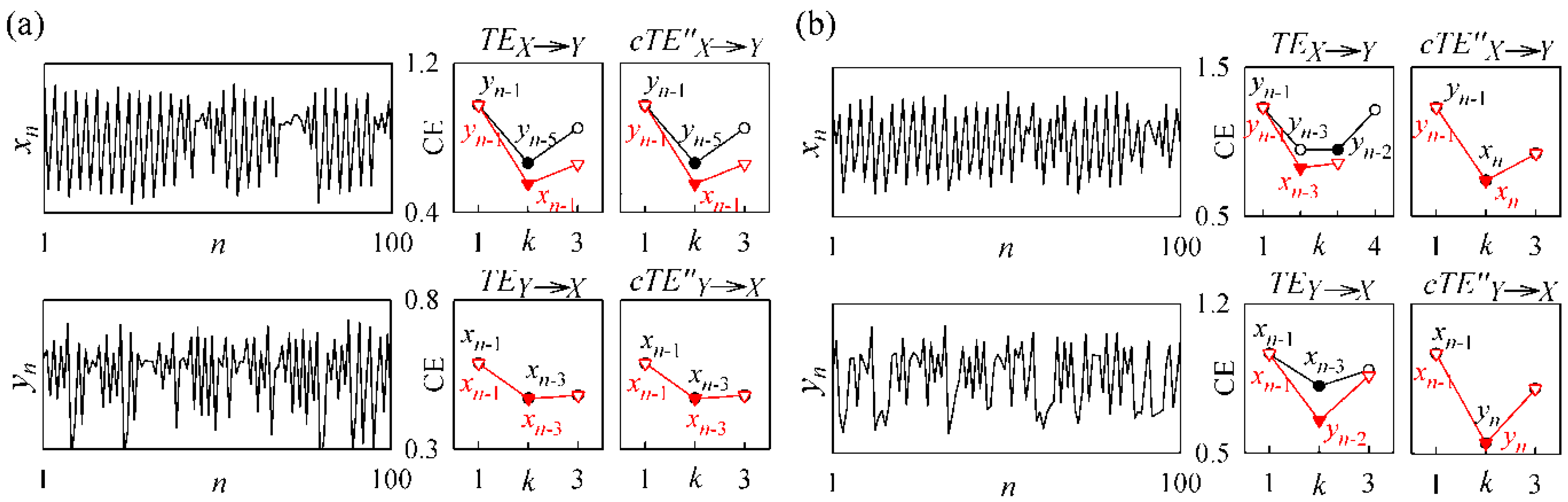
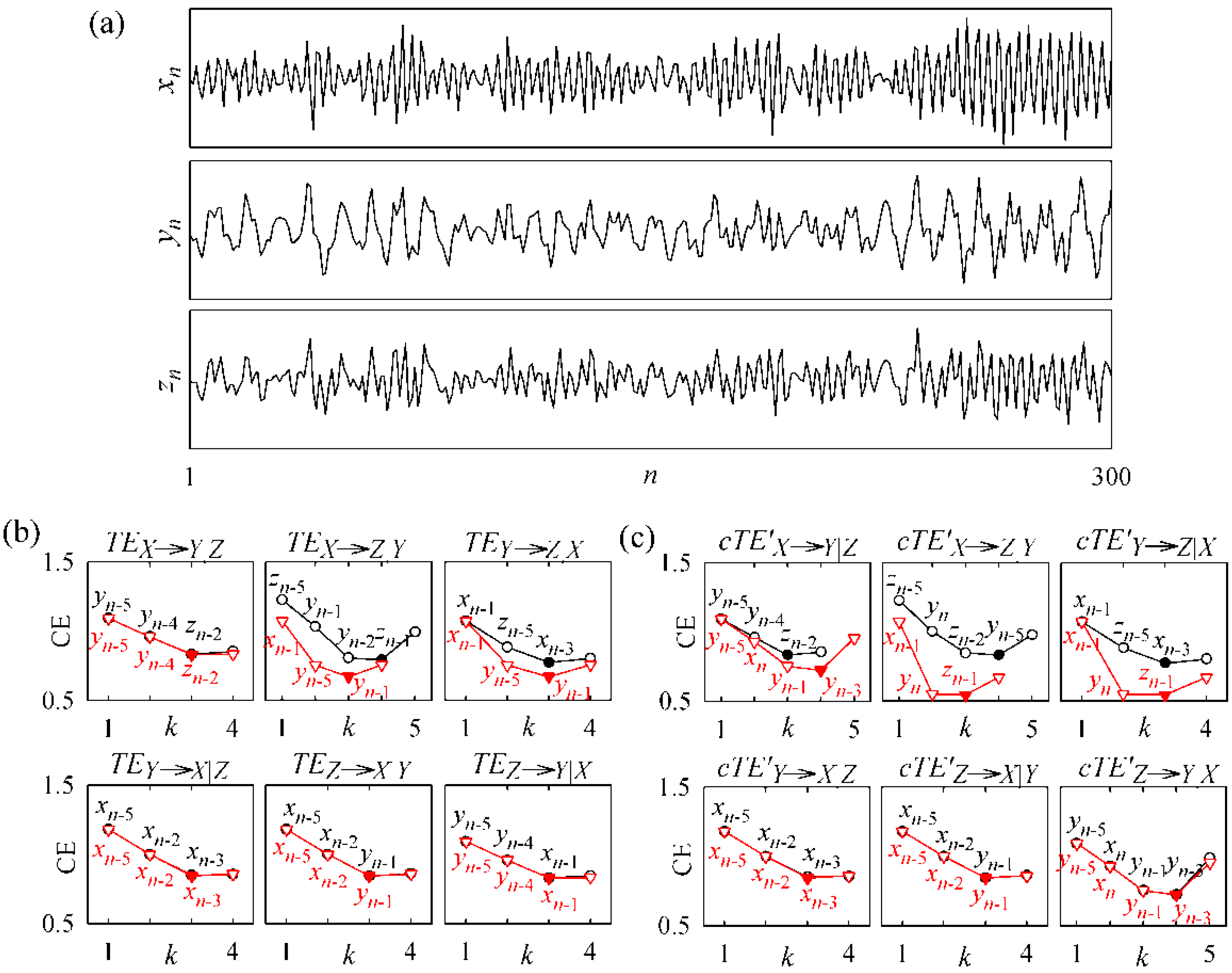
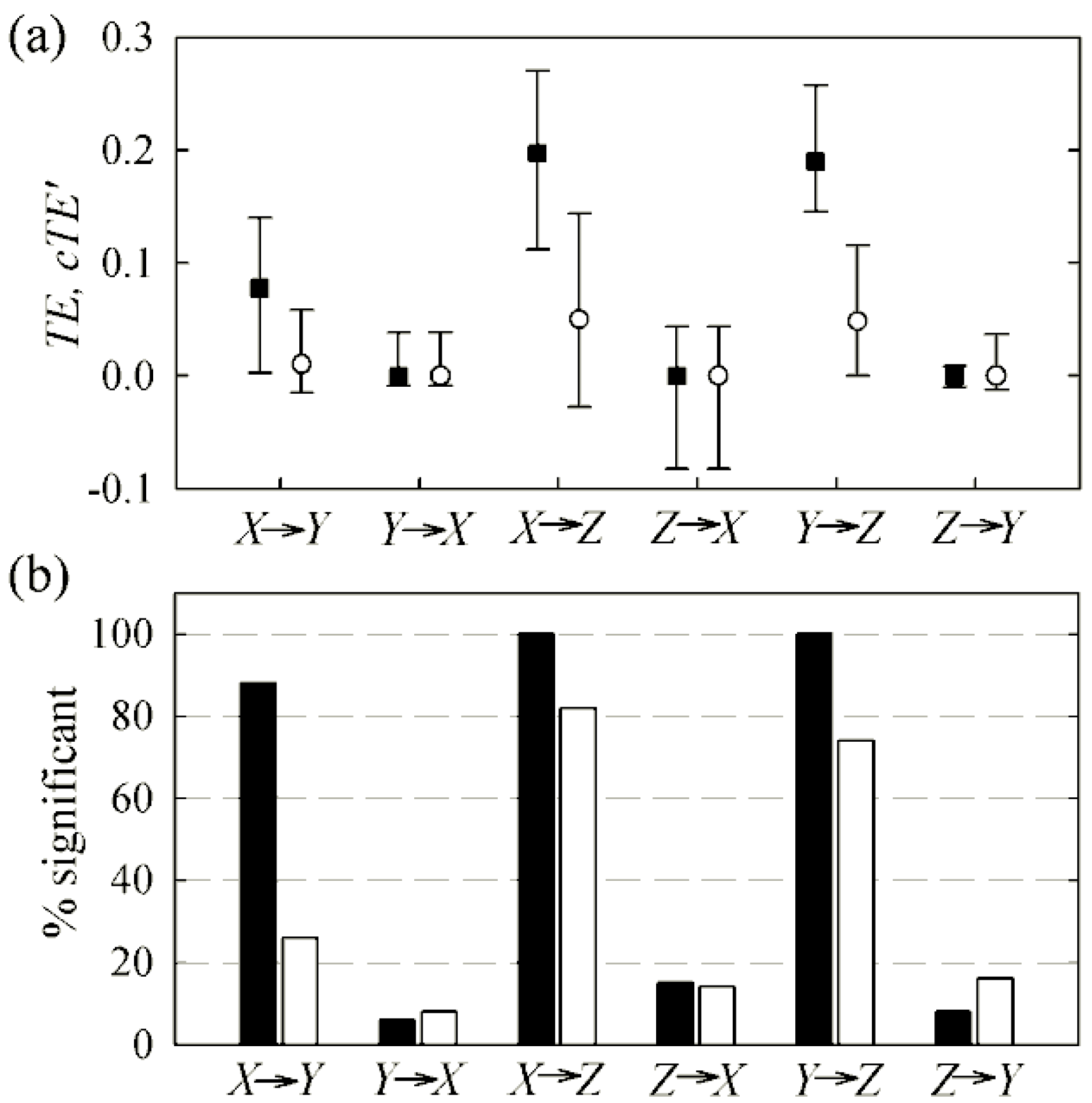
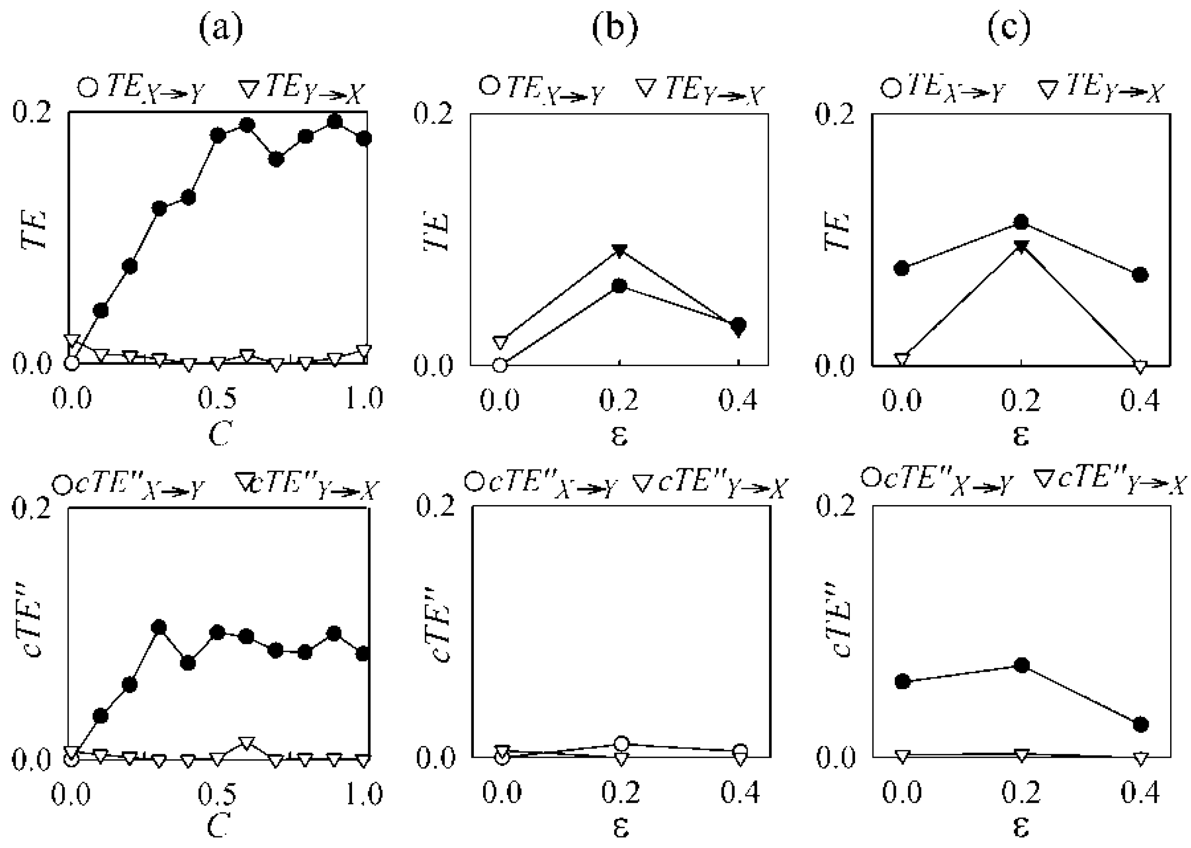
The practical estimation of TE and cTE from finite length realizations of multiple processes faces the issue of reconstructing the state space of the observed multivariate dynamical system and then estimating probabilities within this multidimensional state space. In the context of TE/cTE estimation, state space reconstruction corresponds to identifying the multidimensional vector which more suitably represents the trajectory of the states visited by the composite system {X,Y,Z}. The most commonly followed approach is to perform uniform time delay embedding, whereby each scalar process is mapped into trajectories described by delayed coordinates uniformly spaced in time [29]. In this way the past history of the source process, x_1:n-1, is approximated with the d-dimensional delay vector [x_n-u-(d-1)τ, ..., x_n-u-τ, x_n-u], with τ and u representing the so-called embedding time and prediction time. This procedure suffers from many disadvantages: first, univariate embedding whereby coordinate selection is performed separately for each process does not guarantee optimality of the reconstruction for the multivariate state space [30]; second, selection of the embedding parameters d, τ and u is not straightforward, as many competing criteria exist which are all heuristic and somewhat mutually exclusive [31]; third, the inclusion of irrelevant coordinates consequent to the use of an uniform embedding exposes the reconstruction procedure to the so called “curse of dimensionality”, a concept related to the sparsity of the available data within state spaces of increasing volume [32]. All these problems become more cumbersome when the available realizations are of short length, as commonly happens in physiological time series analysis due to lack of data or stationarity requirements. To counteract these problems, we describe in the following a TE/cTE estimation strategy based on the utilization of a non-uniform embedding procedure combined with a corrected CE estimator [15].

The basic idea underlying our estimation approach is to optimize the time-delay embedding to the estimation of CE, according to a sequential procedure which updates the embedding vector progressively, taking all relevant processes into consideration at each step and selecting the components that better describe the destination process. Specifically, a set of candidate terms is first defined including the past states (and, when relevant, also the present state) of all systems relevant to the estimation of the considered CE term; for instance, considering the terms in (4), the candidate set for the estimation of H(y_n|y_1:n-1,z_1:n) will be the set Ω₁ = {y_n-1,...,y_n-L,z_n,z_n-1,...,z_n-L}, and the candidate set for the estimation of H(y_n|x_1:n, y_1:n-1,z_1:n) in (4) will be the set Ω₂ = {Ω₁,x_n,x_n-1,...,x_n-L} (L is the number of time lagged terms to be tested for each scalar process). Given the generic candidate set Ω, the procedure for estimating the CE H(y_n|Ω) starts with an empty embedding vector V₀ = [·], and proceeds as follows: (i) at each step k ≥ 1, form the candidate vector [s,V_k-1], where s is an element of Ω not already included in V_k-1, and compute the CE of the destination process Y given the considered candidate vector, H(y_n|[s,V_k-1]); (ii) repeat step (i) for all possible candidates, and then retain the candidate for which the estimated CE is minimum, i.e., set V_k = [s′,V_k-1] where s′ = arg min_s H(y_n|[s,V_k-1]); (iii) terminate the procedure when irrelevant terms begin to be selected, i.e. when the decrease of CE is no longer significant; according to the estimation procedure detailed below, this corresponds to stop the iterations at the step k′ such that H(y_n|V_k′) ≥ H(y_n|V_k′-1), and set V_K = V_k′-1 as embedding vector. With this procedure, only the components that effectively contribute to resolving the uncertainty of the target process (in terms of CE reduction) are included into the embedding vector, while the irrelevant components are left out. This feature, together with the termination criterion which prevents the selection of new terms when they do not bring further resolution of uncertainty for the destination process, help escaping the curse of dimensionality for multivariate CE estimation. Moreover the procedure avoids the nontrivial task of setting the embedding parameters (the only parameter is the number L of candidates to be tested for each process, which can be as high as allowed by the affordable computational times). It is worth noting that the proposed sequential procedure for candidate selection takes into account one term at a time, somehow disregarding joint effects that more candidates may have on CE reduction. As a consequence, the sequential instead of exhaustive strategy does not guarantee convergence to the absolute minimum of CE, and thus does not assure a semipositive value for the TE/cTE measures estimated according to (3), (4) and (5). However a sequential approach is often necessary in practical analysis, since exhaustive exploration of all possible combinations of candidate terms would become computationally intractable still at low embedding dimensions.

The application of the procedure described above relies on an efficient estimation of the CE. The problem amounts to estimating, at the k-th step of the procedure, the entropy of the scalar variable y_n conditioned to the vector variable V_k, seen as the difference of two Shannon entropies: H(y_n|V_k) = H(y_n,V_k) − H(V_k). A major problem in estimating CE is the bias towards zero which affects the estimates as the dimension of the reconstructed state space grows higher [33,34]. Since the bias increases progressively with the embedding dimension, its occurrence also prevents from being able to reveal the inclusion of irrelevant terms into the embedding vector by looking at the estimated CE; in other words, since the estimated CE decreases progressively as a result of the bias rather than of the inclusion of relevant terms, the iterations of the sequential procedure for nonuniform embedding cannot be properly stopped. To deal with this important problem, we propose to compensate the CE bias adding a corrective term as proposed by Porta et al. [28,34], in order to achieve a minimum in the estimated CE which serves as stopping criterion for the embedding procedure. The idea is based on the consideration that, for time series of limited length, the CE estimation bias is due to the isolation of the points in the k-dimensional state space identified by the vectors V_k; such an isolation becomes more and more severe as the dimension k increases. Since isolated points tend to give the same contribution to the two entropy terms forming CE (i.e., p(V_k) ≈ p(y_n,V_k) if V_k is an isolated point), their contribution to the CE estimate will be null; therefore, the CE estimate decreases progressively towards zero at increasing the embedding dimension [i.e., when k is high compared to the series length, H(V_k) ≈ H(y_n,V_k) and thus H(y_n|V_k) ≈ 0], even for completely unpredictable processes for which conditioning should not decrease the information carried. This misleading indication of predictability in the analysis of short time series is counteracted introducing a corrective term for the CE. The correction is meant at quantifying the fraction of isolated points V_k in the k-dimensional state space, denoted as n(V_k), and on substituting their null contribution with the maximal information amount carried by a white noise with the same marginal distribution of the observed process y_n [i.e., with H(y_n)]. The resulting final estimate is obtained adding the corrective term n(V_k)H(y_n) to the estimated CE H(y_n|V_k). In the present study, practical implementation of the correction is performed in the context of entropy estimation through uniform quantization [15,28,34]. Briefly, each time series is coarse grained spreading its dynamics over Q quantization levels, so that the state space containing the vectors V_k is partitioned in Q^k disjoint hypercubes. As all points falling within the same hypercube are considered indistinguishable to each other, the Shannon entropy is estimated approximating the probabilities with the frequency of visitation of the hypercubes. Partitioning in disjoint hypercubes helps also in quantifying the fraction of isolated points n(V_k), which is taken simply as the fraction of points found only once inside the hypercubes.

3. Validation

In this section we test the compensation for instantaneous causality in TE computation proposed in Section 2.2, as well as the approach for CE estimation described in Section 2.3, on numerical simulations reproducing different conditions of interaction between multivariate processes. The proposed simulations were devised, in terms of imposed dynamics, interaction conditions and series length, to mimic the conditions typical of the two applicative contexts which are then considered in Section 4, i.e., short-term cardiovascular variability and magnetoencephalography. The reader is referred to [15,28,34] for more extensive validations which investigate the dependence of CE measures on a variety of dynamics, series length, noise conditions, and parameter settings. Here, we consider short realizations of linear stochastic and nonlinear deterministic coupled systems with and without instantaneous effects, and compare TE and cTE as regards their ability to detect the absence or presence of information transfer between pairs of systems. All TE and cTE computations were performed following the described procedure for nonuniform embedding, including in the initial set of candidates L = 10 past terms for each process (plus the zero-lag term when relevant); this choice was based on the necessity to cover the whole range of expected time lagged interactions, while at the same time keeping reasonably low the computational times. The number of quantization levels used for coarse-graining the dynamics of each process was set at Q = 6, in accordance with previous validation studies [15,28,34]; whereas in theory high values of Q would lead to finer state space partitions and more accurate TE estimates, in practice Q should remain as low as Q^K ≈ N for series of length N (with K the embedding dimension) [15,28,34].

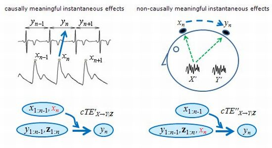
3.1. Physiologically Meaningful Instantaneous Causality

In the first simulation we considered the case in which instantaneous effects are causally meaningful, i.e., correspond to real causal effects between pairs of processes. While zero-lag causal effects are unattainable in physical systems because interactions take time to occur, in practical analysis instantaneous causality becomes meaningfully relevant when the time resolution of the measurements is lower than the time scale of the lagged effects occurring between the processes, or when the time series are built in a way that entails the existence of zero-lag effects. Situations like these are commonly modeled in the framework of Bayesian networks or structural vector autoregression models [18,23,35]. Within this context, we consider a simulation scheme with M = 3 linear stochastic processes X, Y, and Z which interact according to the equations:

$$\begin{array}{l}{x}_n=a_1{x}_{n-1}+a_2{x}_{n-2}+u_n\\ y_n=b_1{y}_{n-1}+b_2{y}_{n-2}+c{x}_n-c{x}_{n-1}+v_n\\ z_n=c{y}_n+c{x}_{n-1}+w_n\end{array}$$

(6)

where u_n, v_n and w_n are independent white noises with zero mean and variance σ²_u = 5, σ²_v = 1, and σ²_w = 1. According to (6), the processes X and Y are represented as second order autoregressive processes described by two complex-conjugate poles with modulus ρ_x,y and phases φ_x,y = ±2πf_x,y; setting modulus and central frequency of the poles as ρ_x = 0.95, ρ_y = 0.92, f_x = 0.3, f_y = 0.1, the parameters quantifying the dependence of x_n and y_n on their own past in (6) are a₁ = 2ρ_xcosφ_x = 0.5871, a₂ = −ρ²_x = −0.9025, b₁ = 2ρ_ycosφ_y = 1.4886, a₂ = −ρ²_y = −0.8464. The other parameters, all set with a magnitude c = 0.5, identify causal effects between pairs of processes; the imposed effects are mixed instantaneous and lagged from X to Y, exclusively instantaneous from Y to Z, and exclusively lagged from X to Z. With this setting, self-dependencies and causal effects are consistent with rhythms and interactions commonly observed in cardiovascular and cardiorespiratory variability, showing an autonomous oscillation at the frequency of the Maier waves (f_y ~ 0.1 Hz) for Y, which is transmitted to Z mimicking feedback effects from arterial pressure to heart period, and an oscillation at a typical respiratory frequency (f_x ~ 0.3 Hz) for X, which is transmitted to both Y and Z mimicking respiratory-related effects on arterial pressure and heart period (a realization of the three processes is shown in Figure 1a).

The analysis was performed on 100 realizations of (6), each lasting N = 300 points. For each realization, we computed the TE according to (3) and the cTE according to (4). The statistical significance of each estimated information transfer was assessed by using surrogate time series. Specifically, the TE or cTE of the original time series was compared with the distribution of its values obtained for a set of S = 40 realizations of time-shifted surrogates, obtained by shifting the source time series of a randomly selected lag (>20 points); then, the null hypothesis of absence of information transfer was rejected if the original TE or cTE took the first or second position in the descending ordered sequence of original and surrogate values (this corresponds to a type-I error probability of 0.0405 [36]).

An example of the analysis is depicted in Figure 1. Each panel reports the corrected CE estimated for the destination process after conditioning to all processes except the source process (black) and after conditioning to all processes including the source process (red), together with the term selected at each step of the conditioning procedure. Note that the two estimated CE profiles overlap whenever no terms from the source process are selected even if considered as possible candidates, so that the two CE minima are the same and the estimated TE or cTE is zero. For instance, considering the estimation of TE or cTE from Y to X conditioned to Z (lower left panel in Figure 1b,c) we see that the first repetition of the embedding procedure –which starts from the initial set of candidate terms Ω₁ = {x_n-1,...,x_n-10, z_n-1,...,z_n-10} − selects progressively the past terms of X with lags 5, 2, and 3, terminating at the third step with the embedding vector V₃ = [x_n-5, x_n-2, x_n-3]. The second repetition of the procedure, although starting with the enlarged set of candidates Ω₂ = {Ω₁,y_n-1,...,y_n-10,} which includes also past terms from the source system Y, selects exactly the same candidates leading again to the embedding vector V₃ = [x_n-5, x_n-2, x_n-3] and yielding no reduction in the estimated CE minimum, so that we have TE_Y→X|Z = cTE′_Y→X|Z = 0.

Figure 1. Example of transfer entropy analysis performed for the first simulation. (a) realization of the three processes generated according to (6). (b) TE estimation between pairs of processes based on nonuniform embedding; each panel depicts the CE estimated for the destination process through application of the non-uniform embedding procedure without considering the source process (black circles), or considering the source process (red triangles), in the definition of the set of candidates; the terms selected at each step k of the sequential embedding are indicated within the plots, while filled symbols denote each detected CE minimum. (c) Same of (b) for estimation of the compensated TE (cTE′).

Figure 1. Example of transfer entropy analysis performed for the first simulation. (a) realization of the three processes generated according to (6). (b) TE estimation between pairs of processes based on nonuniform embedding; each panel depicts the CE estimated for the destination process through application of the non-uniform embedding procedure without considering the source process (black circles), or considering the source process (red triangles), in the definition of the set of candidates; the terms selected at each step k of the sequential embedding are indicated within the plots, while filled symbols denote each detected CE minimum. (c) Same of (b) for estimation of the compensated TE (cTE′).

On the contrary, the selection of one or more terms from the input process during the second repetition of the procedure leads to a decrease in the CE minimum, and thus to the detection of a positive information transfer. For instance, considering the estimation of TE from Y to Z conditioned to X (upper right panel in Figure 1b) the vector resulting from the first embedding is [x_n-1, z_n-5, x_n-3], while the second embedding selects at the second and third steps some past terms from the source process Y (i.e., the terms y_n-5 and y_n-1), so that the selected embedding vector changes to [x_n-1, y_n-5, y_n-1] and this results in a reduction of the CE minimum with respect to the first embedding and in the detection of a nonzero information transfer (TE_Y→Z|X > 0).

The difference between TE and cTE is in the fact that in cTE computation the zero-lag term of the source process is a possible candidate in the second repetition of the embedding procedure, so that when selected to enter the embedding vector, it may reduce the information carried by the target process and thus lead to detecting information transfer. In the example of Figure 1, this is the case of the analysis performed from X to Y: the traditional TE misses detection of the existing information transfer because the procedure selects at both repetitions the embedding vector [y_n-5, y_n-4, z_n-2], failing to include any term from the source system X and thus returning TE_X→Y|Z = 0 (Figure 1b, upper left panel); on the contrary the compensated TE captures the information transfer thanks to the fact that the zero-lag term x_n is in the set of candidates for the second embedding, and is selected determining a reduction in the estimated CE that ultimately leads to cTE′_X→X|Z > 0 [Figure 1c, upper left panel].

Figure 2 reports the results of the analysis extended to all realizations. As seen in Figure 2a, the distributions of both TE and cTE′ are close to zero when computed over the directions for which no information transfer was imposed (i.e., Y→X, Z→X and Z→Y), and cover a range of larger positive values over the directions with imposed coupling (X→Y, X→Z and Y→Z). cTE′ shows higher values than TE when computed over the coupled directions, while the two distributions substantially overlap when evaluated over the uncoupled directions. Note that markedly higher values are obtained for cTE′ compared to TE even for the direction X→Z even though X does not contribute to Z in an instantaneously causal way; this is likely due to the fact that Y causes Z instantaneously, an effect that cannot be detected in the traditional analysis and ultimately leads to underestimation of the TE.

Figure 2. Results of transfer entropy analysis for the first simulation. (a) Distribution over 100 realizations of (6) (expressed as 5th percentile, median and 95th percentile) of the information transfer estimated between each pair of processes using the traditional TE (white) and the compensated TE (black). (b) Percentage of realizations for which the information transfer estimated using TE (white) and compensated TE (black) was detected as statistically significant according to the test based on time-shifted surrogates.

Figure 2. Results of transfer entropy analysis for the first simulation. (a) Distribution over 100 realizations of (6) (expressed as 5th percentile, median and 95th percentile) of the information transfer estimated between each pair of processes using the traditional TE (white) and the compensated TE (black). (b) Percentage of realizations for which the information transfer estimated using TE (white) and compensated TE (black) was detected as statistically significant according to the test based on time-shifted surrogates.

The results of Figure 2a are further supported by the percentage of significant information transfer of Figure 2b. Indeed, while over the uncoupled directions the number of detected significant causal couplings is low and comparable for TE and cTE′ (the overall specificity is 87% for the TE and 90% for the cTE), over the coupled directions the number of detected significant couplings is substantially higher for cTE′ than for TE (the overall sensitivity is 61% for the TE and 96% for the cTE). Thus, in this situation with causally meaningful instantaneous interactions, utilization of the cTE in place of the traditional TE yields a better sensitivity in the detection of information transfer between coupled processes.

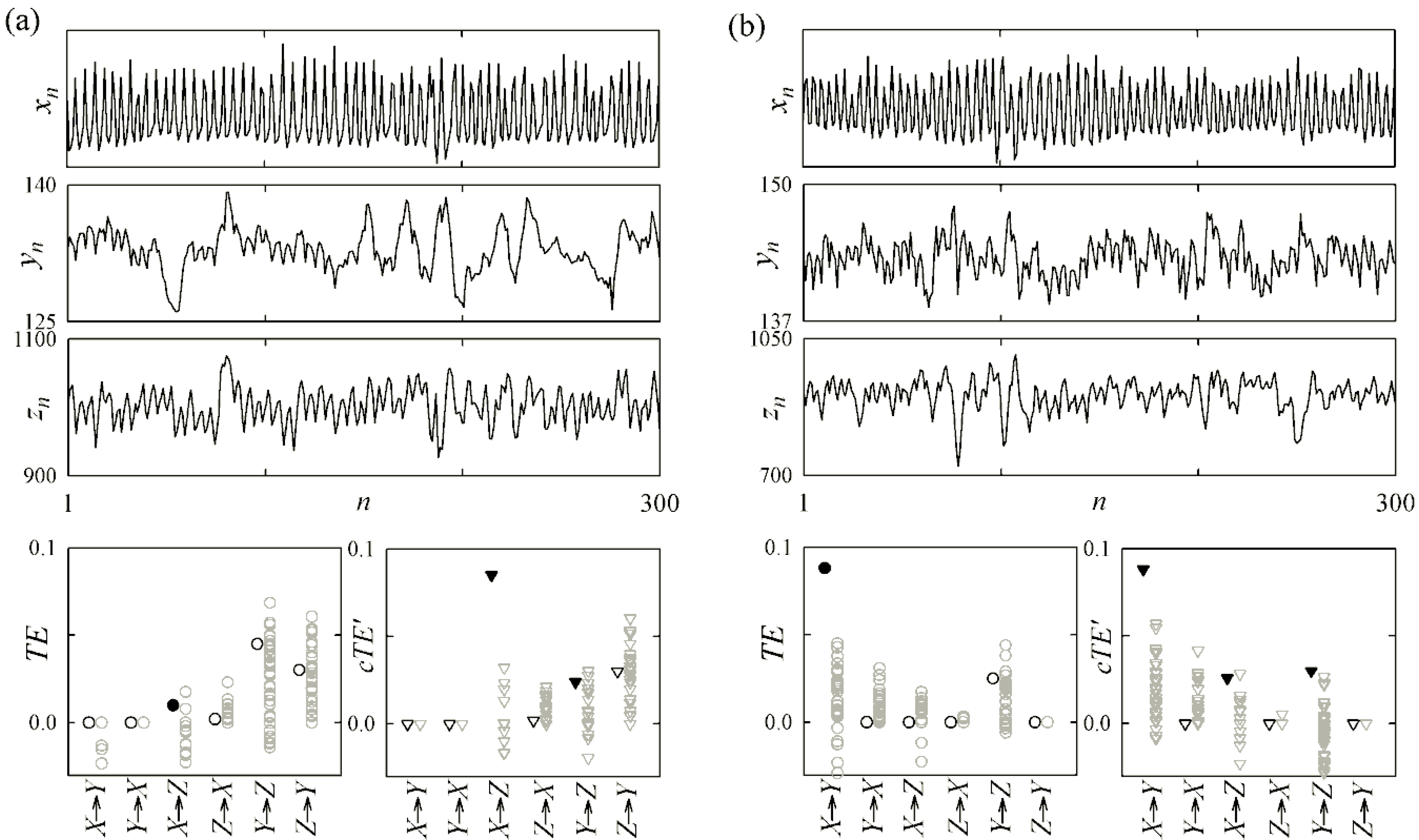
3.2. Non-Physiological Instantaneous Causality

In the second simulation we considered the case in which instantaneous effects are not physiologically meaningful, reproducing a situation of cross-talk between two nonlinear processes which is typical in the analysis of neurophysiological settings where data acquired at the scalp level are the result of the instantaneous mixing of unmeasured cortical sources. Specifically, we considered the simulated systems X′ and Y′ described by two unidirectionally coupled logistic processes x′ and y′:

$$\begin{array}{l}{x}_n^{\prime }=R_1{x}_{n-1}^{\prime }\left(1-x_{n-1}^{\prime }\right)\\ y_n^{\prime }=C{x}_{n-1}^{\prime }+\left(1-C\right)\left[R_2{y}_{n-1}^{\prime }\left(1-y_{n-1}^{\prime }\right)\right]\end{array}$$

(7)

which were then instantaneously mixed to obtain the processes x and y as:

$$\begin{array}{l}{x}_n=\left(1-\epsilon \right)x_n^{\prime }+\epsilon \text{}{y}_n^{\prime }+u_n\\ y_n=\epsilon \text{}{x}_n^{\prime }+\left(1-\epsilon \right)\text{}{y}_n^{\prime }+w_n\end{array}$$

(8)

where u and w are independent additive noise processes with zero mean and variance set to get a signal-to-noise ratio of 20 dB. In (7), we set R₁ = 3.86 and R₂ = 4 to obtain a chaotic behavior for the two logistic maps describing the autonomous dynamics of X and Y; the parameters C and ε in (7) and (8) set respectively the strength of coupling from X to Y and the amount of instantaneous mixing between the two processes.

The analysis was performed at varying the coupling strength from C = 0 (absence of coupling) to C = 1 (full coupling, intended as absence of self-dependencies in Y with maximal dependence on X) in the absence of signal mixing (ε = 0), and at varying the mixing parameter from ε = 0 to ε = 0.4 either in the absence of coupling (C = 0) or with fixed coupling (C = 0.2). For each combination of the parameters, 50 realizations of (7-8) were generated, each lasting 100 points, and the TE and cTE were computed according to (3), (4) and (5), respectively. Since in this simulation the data were interpreted as having a trial structure, as typically happens in neurophysiological studies, the statistical significance of each estimated information transfer was assessed by means of a permutation test. The test consisted in performing repeatedly (S = 100 times in this study) a random shuffling of the relative ordering of the trials for the two processes to get S datasets with uncoupled trials; then, the null hypothesis of absence of information transfer was rejected if the median TE (or cTE′′) computed for the original trials was outside the 95-th percentile of the distribution of the median TE (or cTE′′) computed over the S datasets with shuffled trials (this corresponds to set a type-I error probability of 0.05).

Examples of the analysis performed with significant coupling but absence of signal cross-talk (C = 0.2, ε = 0) and significant cross-talk but absence of coupling (C = 0, ε = 0.2) are depicted in Figure 3a,b, respectively. In the first case, both TE and cTE seem able to detect correctly the imposed unidirectional coupling. Indeed, in the computation of TE_X→Y and cTE′′_X→Y the second repetition of the conditioning procedure (red) selects a term from the input process (i.e., x_n-1) determining a decrease in the estimated CE minimum and thus the detection of a positive information transfer; on the contrary, the analysis performed from Y to X does not select any term from the source process in the second repetition of the conditioning procedure, thus leading to unvaried CE and hence to null values of the information transfer (TE_Y→X = cTE′′_Y→X = 0). The identical behavior of TE and cTE is explained by noting that, in this case with absence of instantaneous signal mixing, zero-lag effects are not present, and indeed the zero-lag term is not selected (although tested) during the embedding procedures for cTE. On the contrary, in the case of Figure 3b where the instantaneous mixing is not trivial, the two repetitions of the embedding procedure for cTE both select the zero lag-term (x_n in the analysis from X to Y and y_n in the analysis from Y to X); as a consequence, the cTE correctly reveals the absence of information transfer from X to Y and from Y to X, while the TE seems to indicate a false positive detection of information transfer over both directions because of the CE reduction determined by inclusion of a term from the input process during the second conditioning.

Figure 3. Example of transfer entropy analysis performed for the second simulation. (a) Presence of coupling and absence of instantaneous mixing (C = 0.2, ε = 0) (b) Absence of coupling and presence of instantaneous mixing (C = 0, ε = 0.2). Panels depict a realization of the two processes X and Y generated according to (7) and (8), together with the estimation of TE and cTE′′ over the two directions of interaction based on nonuniform embedding and conditional entropy (CE, see caption of Figure 1 for details).

Figure 3. Example of transfer entropy analysis performed for the second simulation. (a) Presence of coupling and absence of instantaneous mixing (C = 0.2, ε = 0) (b) Absence of coupling and presence of instantaneous mixing (C = 0, ε = 0.2). Panels depict a realization of the two processes X and Y generated according to (7) and (8), together with the estimation of TE and cTE′′ over the two directions of interaction based on nonuniform embedding and conditional entropy (CE, see caption of Figure 1 for details).

Figure 4 reports the results of the overall analysis. As shown in Figure 4a, the traditional and compensated TE perform similarly in the absence of signal cross-talk, as the median values of TE and cTE′′ are statistically significant, according to the permutation test, for all values of C > 0 when computed from X to Y, and are never statistically significant when computed from Y to X. On the contrary, the presence of instantaneous mixing may induce the traditional TE to yield a misleading indication of information transfer for uncoupled processes. This erroneous indication occurs in Figure 4b where both TE_X→Y and TE_Y→X are statistically significant with ε>0 even though X and Y are uncoupled over both the directions of interaction, and in Figure 4c where TE_Y→X is statistically significant with ε = 0.2 even though no coupling was imposed from Y to X (in total, false positive detections using the TE were five out of six negative cases with presence of instantaneous mixing). Unlike the traditional TE, the cTE does not take false positive values in the presence of signal cross-talk, as the detected information transfer is not statistically significant over both directions in the case of uncoupled systems of Figure 4b, and is statistically significant from X to Y but not from Y to X in the case of unidirectionally coupled systems of Figure 4c. Thus, in this simulation where instantaneous causality is due to common driving effects, utilization of cTE′′ in place of the traditional TE measure yields a better specificity in the detection of predictive information transfer.

Figure 4. Results of transfer entropy analysis for the second simulation, showing the median values over 50 realizations of (7) and (8) of the TE (first panel row) and the compensated TE (second panel row) computed along the two directions of interactions (X→Y, circles; Y→X, triangles) (a) at varying the parameter C with parameter ε = 0; (b) at varying ε with C = 0 (b); and (c) varying ε with C = 0.2. Filled symbols denote statistically significant values of TE or cTE′′ assessed by means of the permutation test.

Figure 4. Results of transfer entropy analysis for the second simulation, showing the median values over 50 realizations of (7) and (8) of the TE (first panel row) and the compensated TE (second panel row) computed along the two directions of interactions (X→Y, circles; Y→X, triangles) (a) at varying the parameter C with parameter ε = 0; (b) at varying ε with C = 0 (b); and (c) varying ε with C = 0.2. Filled symbols denote statistically significant values of TE or cTE′′ assessed by means of the permutation test.

4. Application Examples

This section describes the evaluation of the proposed TE/cTE estimation approach in physiological systems where commonly only short realizations of the studied processes (few hundred points) are available due to stationarity constraints. The considered applications are taken as examples of commonly performed time series analyses of physiological systems, i.e., the study of short-term cardiovascular and cardiorespiratory interactions during a paced breathing protocol [7], and the study of neural interactions from magnetoencephalographic data during an experiment of visuo-motor integration [37].

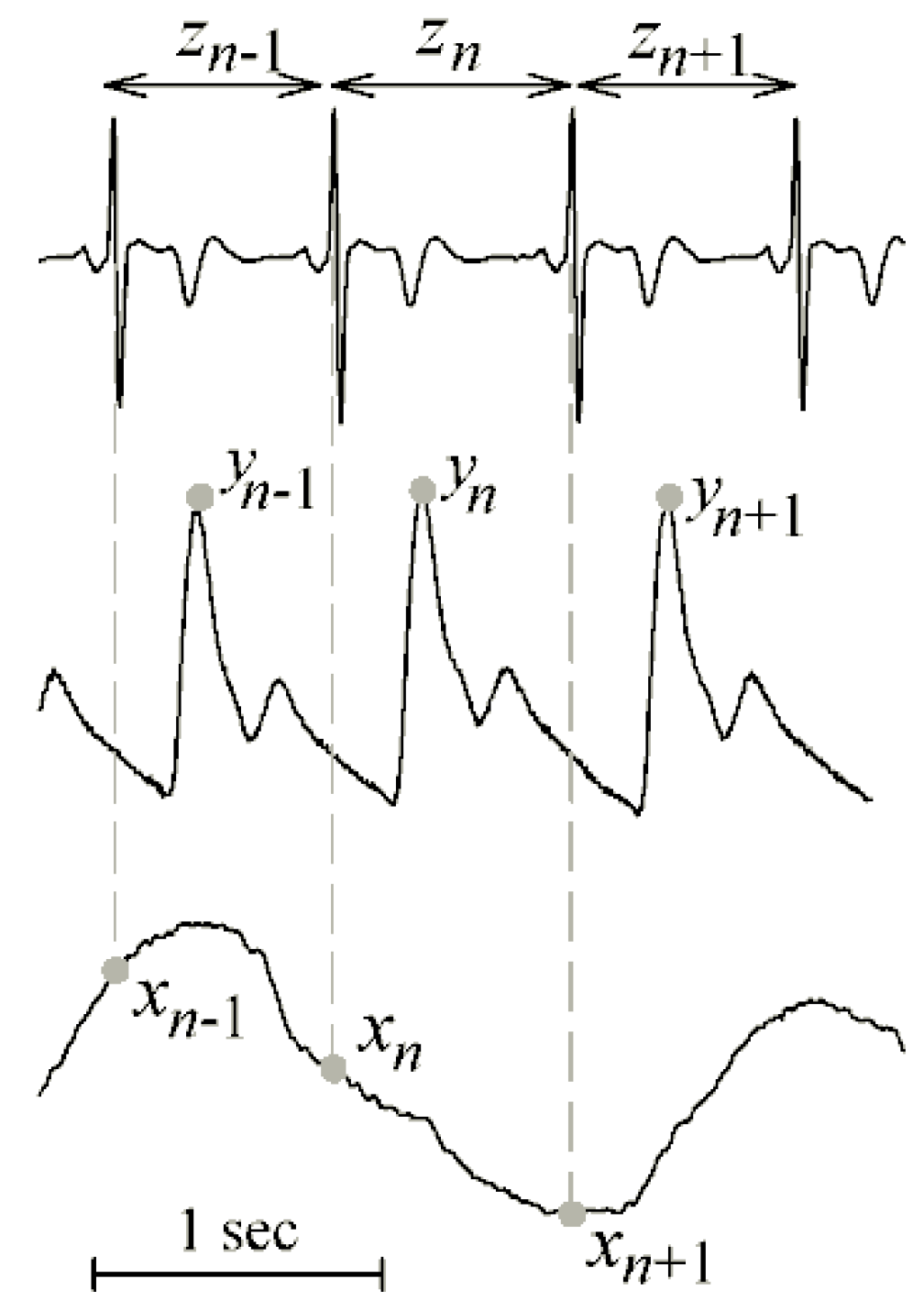
4.1. Cardiovascular and Cardiorespiratory Variability

In the first application we studied cardiovascular and cardiorespiratory time series measured during an experiment of paced breathing [7]. The considered dynamical systems are the respiratory system, the vascular system, and the cardiac system, from which we take the respiratory flow, the systolic arterial pressure and the heart period as representative processes, respectively denoted as processes x, y and z. Realizations of these processes were obtained measuring in a healthy subject the beat-to beat time series of heart period, z_n, systolic pressure, y_n,, and respiratory flow, x_n, respectively as the sequences of the temporal distances between consecutive heartbeats detected from the electrocardiogram, the local maxima of the arterial pressure signal (acquired through the Finapres device) measured inside each detected heart period, and the values of the airflow signal (acquired from the nose through a differential pressure transducer) sampled at the onset of each detected heart period. The measurement convention is illustrated in Figure 5. The experimental protocol consisted in signal acquisition, after subject stabilization in the resting supine position, for 15 min with spontaneous breathing, followed by further 15 min with the subject inhaling and exhaling in time with a metronome acting at 15 cycles/min (paced breathing at 0.25 Hz). Two artifact-free windows of N = 300 samples, measured synchronously for the M = 3 series during spontaneous breathing and during paced breathing, were considered for the analysis. Weak stationarity of each series was checked by means of a test checking the stability of the mean and variance over the analysis window [38]. The analyzed series are shown in Figure 6.

Figure 5. Measurement of heart period (series z), systolic arterial pressure (series y) and respiratory flow (series x) variability series from the electrocardiogram, arterial blood pressure and nasal flow signals.

Figure 5. Measurement of heart period (series z), systolic arterial pressure (series y) and respiratory flow (series x) variability series from the electrocardiogram, arterial blood pressure and nasal flow signals.

In this application, instantaneous effects between the measured time series were considered as physiologically meaningful, since from the above described measurement convention we can infer that the occurrence of the present respiration value, x_n, precedes in time the occurrence of the present systolic pressure value, y_n, which in turn precedes in time the end of the present heart period, z_n (see Figure 5). Therefore, cTE analysis was performed for this application using the compensation proposed in (4). The statistical significance of each estimated TE and cTE′ was assessed using time shifted surrogates. The results of the analysis for the spontaneous breathing and paced breathing conditions are depicted in Figure 6a,b, respectively. Utilization of the traditional TE led to detect as statistically significant the information transfer measured from respiration to heart period during spontaneous breathing (TE_X→Z in Figure 6a, and from respiration to systolic pressure during paced breathing (TE_X→Y in Figure 6b. The same analysis performed accounting for instantaneous causality effects led to detect a higher number of statistically significant interactions, specifically from respiration to heart period and from systolic pressure to heart period during both conditions (cTE′_X→Z and cTE′_Y→Z in Figure 6a,b), and also from respiration to systolic pressure during paced breathing (cTE′_X→Y in Figure 6b).

Figure 6. Transfer entropy analysis in cardiovascular and cardiorespiratory variability performed. (a) during spontaneous breathing and (b) during paced breathing. Plots depict the analyzed time series of respiratory flow (x_n, system X), systolic arterial pressure (y_n, system Y) and heart period (z_n, system Z) together with the corresponding TE (circles) and compensated TE (triangles) estimated between each pair of series. The gray symbols indicate the values of TE/cTE obtained over 40 pairs of time-shifted surrogates; filled symbols denote statistically significant TE or cTE′.

Figure 6. Transfer entropy analysis in cardiovascular and cardiorespiratory variability performed. (a) during spontaneous breathing and (b) during paced breathing. Plots depict the analyzed time series of respiratory flow (x_n, system X), systolic arterial pressure (y_n, system Y) and heart period (z_n, system Z) together with the corresponding TE (circles) and compensated TE (triangles) estimated between each pair of series. The gray symbols indicate the values of TE/cTE obtained over 40 pairs of time-shifted surrogates; filled symbols denote statistically significant TE or cTE′.

Though not conclusive as they are drawn on a single subject, these results suggest a higher sensitivity of the cTE, compared with the traditional TE, in the detection of information transfers that can be associated to known cardiovascular and cardiorespiratory mechanisms. These mechanisms, also recently investigated using tools based on transfer entropy [7], are the baroreflex modulation of heart rate, manifested through coupling from systolic pressure to heart period variability [39], and the effects of respiration on heart period (describing the so-called respiratory sinus arrhythmia [40]) and on arterial pressure (describing the mechanical perturbations of arterial pressure originating from respiration-related movements [41]). In particular, the higher sensitivity of cTE to the information transferred from systolic pressure to heart period, denoted in this example by the significant values observed for cTE′_Y→Z but not for TE_Y→Z in both conditions, could suggest a major role played by fast vagal effects −whereby the systolic pressure affects heart period within the same heartbeat—in the functioning of the baroreflex mechanism.

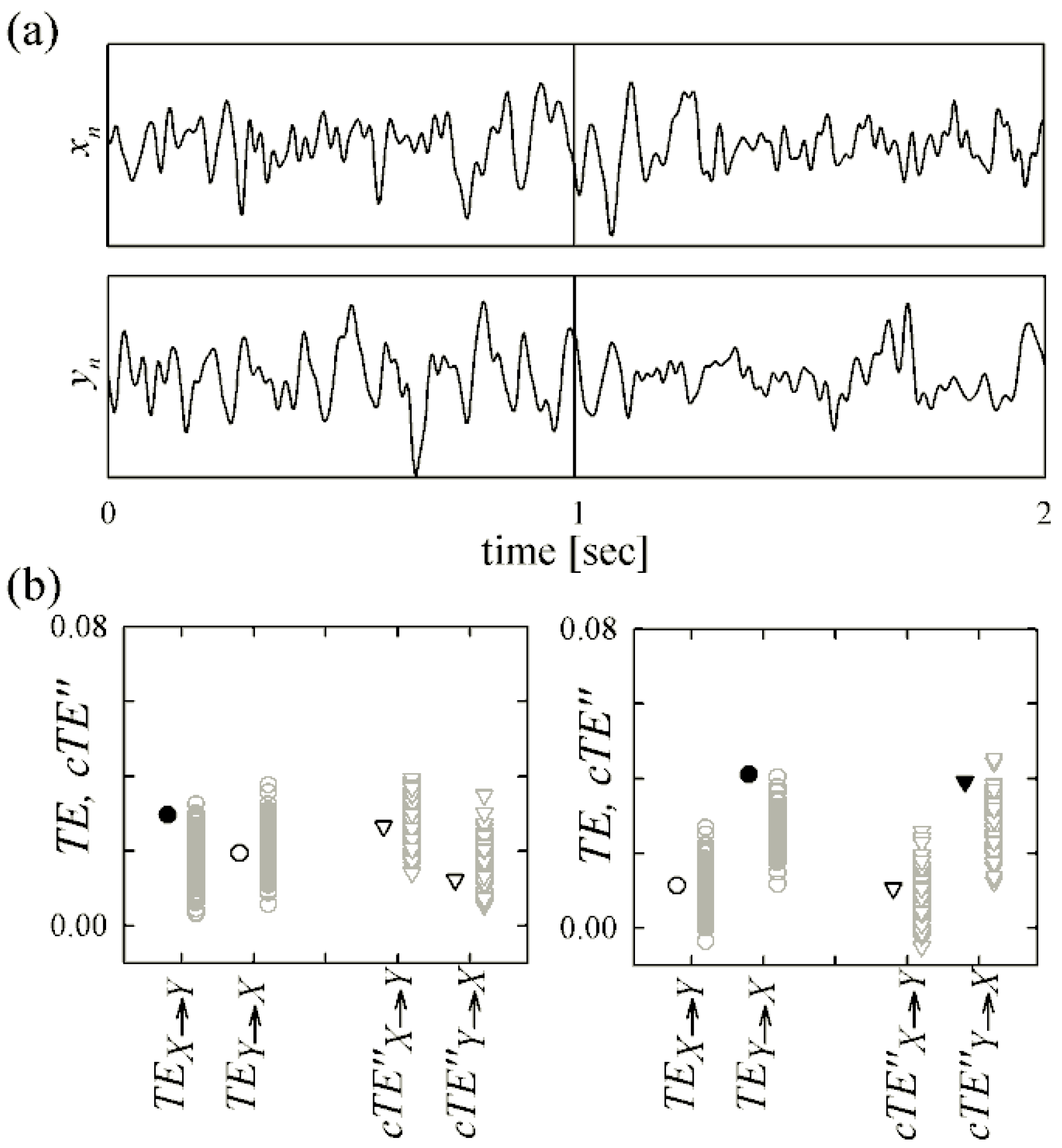
4.2. Magnetoencephalography

The second application is about quantification of the information transfer between different cerebral areas from the analysis of magnetoencephalographic (MEG) data. The analyzed MEG signals were taken from a database of neurobiological recordings acquired during a visuo-tactile cognitive experiment [42]. Briefly, a healthy volunteer underwent a recording session in which simultaneous visual and tactile stimuli were repeatedly presented (60 trials). At each trial, geometric patterns resembling letters of the Braille code were both shown on a monitor and embossed on a tablet, and the subject had to perceive whether the pattern seen on the screen was the same of that touched on the tablet. The MEG signals (VSM whole head system) were recorded with 293 Hz sampling frequency during two consecutive time frames of 1 s, before (rest window) and after (task window) the presentation of the combined stimuli.

The two dynamical systems considered for this application were the somatosensory cortex (system X) and the visual cortex (system Y). At each experimental trial, we considered two MEG sensors as representative of the two areas, and considered the signals measured from these sensors as realizations of the processes x and y. Sensor selection was performed trial by trial through a suitable event-related field analysis looking for the scalp locations, situated within the visual cortex and the somatosensory cortex, at which the signal magnitude was maximized in response to pure-visual or pure-tactile stimulation [42]. The considered signals were preprocessed applying a band-pass filter (FFT filter, 2–45 Hz); moreover, the event-related field was removed from each task window by subtraction of the average response over the 60 trials. An example of the analyzed signals is shown in Figure 7a,b.

Figure 7. Transfer entropy analysis in magnetoencephalography performed before (left) and during (right) presentation of the combined visuo-tactile stimuli. (a) Representative MEG signals acquired from the somatosensory cortex (x_n, system X) and the visual cortex (y_n, system Y) for one of the experiment trials (n ranges from 1 to 293 samples before and during simulation). (b) Median over the 60 trials of TE (circles) and compensated TE (triangles) estimated for the two directions of interaction between X and Y before and during stimulation; gray symbols indicate the values of TE/cTE′′ obtained over 100 trial permutations; filled symbols denote statistically significant TE or cTE′′.

Figure 7. Transfer entropy analysis in magnetoencephalography performed before (left) and during (right) presentation of the combined visuo-tactile stimuli. (a) Representative MEG signals acquired from the somatosensory cortex (x_n, system X) and the visual cortex (y_n, system Y) for one of the experiment trials (n ranges from 1 to 293 samples before and during simulation). (b) Median over the 60 trials of TE (circles) and compensated TE (triangles) estimated for the two directions of interaction between X and Y before and during stimulation; gray symbols indicate the values of TE/cTE′′ obtained over 100 trial permutations; filled symbols denote statistically significant TE or cTE′′.

In this application, instantaneous effects were considered as non-physiological, because in large part they are the result by artifacts of volume conduction, i.e., of the instantaneous mixing of unmeasured cortical sources which are simultaneously mapped onto the different MEG sensors [43]. Therefore, cTE analysis was performed using the compensation for signal cross-talk proposed in (5). The statistical significance of each estimated TE and cTE′′ value was assessed using a permutation test applied to the 60 trials.

The results shown in Figure 7b indicate that the TE is statistically significant from the somatosensory area towards the visual area before stimulus presentation, and from the visual area to the somatosensory area during stimulation. On the other hand, the cTE was not statistically significant along any direction before task, and was significant from the visual area to the somatosensory area during task. Therefore, utilization of cTE′′ seems to indicate in this exemplary application the emergence of causality X→Y with stimulus presentation, with a significant information transfer detected only during execution of the task. This result is compatible with the activation of mechanisms of sensory-motor integration moving from rest to task, with the posterior visual cortex driving the coherent activation of the somatosensory cortex during the combined visuo-tactile stimulation [44]. Moreover, the significant information transfer detected by the traditional TE over the opposite direction in the absence of stimulation, which is more difficult to interpret according to the paradigm proposed by this experiment, could be interpreted as a false positive detection of information transfer, thus confirming the lower specificity of non-compensated TE analysis evidenced by the simulation results. While the results reported here are certainly not conclusive, we believe that utilization of a nonlinear, model-free tool like TE, in conjunction with the compensation for instantaneous mixing realized by cTE, may deepen the interpretation of the mechanisms of multisensory integration involved in visuo-tactile experiments given by more standard tools, e.g., based on spectral analysis [37,42].

5. Discussion

Our results suggest that the framework proposed in this study for the practical estimation of multivariate TE can successfully deal with the issues arising in the conditions typical of physiological time series analysis. First, to counteract the problems related to high dimensionality and small sample size, we exploited a data-efficient estimation approach which combines a strategy for optimizing the embedding of multiple time series with a method for correcting the bias that affect conditional entropy estimates progressively at increasing the embedding dimension [15]. The reported simulation results indicate that using this approach together with appropriate statistical tests (i.e., time-shifted surrogates or, when the dataset has a trial structure, permutation tests), detection of significant information transfer is possible even when the analyzed realizations are very short (a few hundred data points). Moreover, we devised a compensation strategy aimed at properly taking into account the concept of instantaneous causality in the computation of TE. In the presented simulated datasets utilization of this strategy led to an improvement in sensitivity of about 35% when instantaneous effects were physiologically meaningful, and to an improvement in specificity of about 85% when instantaneous effects were non physiological (i.e., due to common driving from unobserved sources). These two kinds of improvement were suggested also by the reported representative applications to physiological time series. In cardiovascular and cardiorespiratory variability, where the construction of the time series suggests the existence of physiological causal effects occurring at lag zero, the compensated TE evidenced better than the traditional TE the presence of expected interaction mechanisms (e.g., the baroreflex). In magnetoencephalography, where instantaneous effects are likely the result of the simultaneous mapping of single sources of brain activity onto several recording sensors, utilization of the proposed compensation suggested the activation of multisensory integration mechanisms in response to a specific stimulation paradigm. Nevertheless, we emphasize that practical analysis was limited in the present study to preliminary investigations aimed at supporting the feasibility of the proposed approach in different fields of application, and that systematic tests performed on extensive databases need to be carried out to corroborate the validity of our experimental results.

While with the present study we have proposed feasible approaches to deal with the detrimental effects of instantaneous causality in the practical estimation of TE, it is important to remark that the proposed compensations constitute an empirical rather than a principle solution to the problem. In fact, from a theoretical perspective the compensation achieved in (4) through the index cTE′ could not yield a better sensitivity than the traditional TE measure (3), because an instantaneous causal effect from X to Y can be detected by cTE′ reflecting a direct effect x_n→y_n, but by TE as well reflecting an indirect effect x_1:n-1→x_n→y_n, (provided that X has an internal memory structure). Therefore, the higher sensitivity observed for the cTE in this case should be explained in practical terms (i.e., as an easier estimation of a direct than an indirect effect). Moreover, when instantaneous effects are causally meaningful, including them in TE computation as done in (4) might yield to a detection of information transfer not only over the direction of the actual causal effects, but also over the opposite direction. On the other hand, when instantaneous effects are not causally meaningful the full removal of zero-lag effects performed by (5) may be conservative when real causal effects taking place within the same sample are present besides the spurious effects to be removed. Another point regarding theoretical values of the index cTE′′ is that conditioning to the zero-lag term as done in (5) may cause, in particular circumstances involving unobserved variables (e.g., due to latent confounders or resulting from inappropriate sampling), spurious detections of predictive information transfer reflecting an effect known as “selection bias” or “conditioning on a collider” [45]. Nevertheless it is likely that, in most practical situations in which real short data sequences are considered and significance tests are applied, the null hypothesis of absence of information transfer cannot be rejected solely as a consequence of spurious effects deriving from selection bias. Further studies should be aimed at assessing the real capability of these spurious effects to produce detectable predictive information transfer in practical estimation contexts.

As to the practical utilization of the cTE estimation framework developed in this study, we stress that the proposed compensation for instantaneous causality relies on prior knowledge about the nature of the zero-lag interactions among the observed physiological processes. Indeed, we have shown that the proposed compensation strategies work properly only when one can reasonably assume that instantaneous effects are the result of an improper sampling of actual physiological causal interactions, or of a simultaneous mapping of unobserved processes. In fact, using the index cTE′ when instantaneous effects are not causally meaningful may exacerbate the false positive detection of information transfer, while using cTE′′ in the presence of meaningful instantaneous effects does not improve the detection rate. Therefore, future studies should aim at integrating within our framework recently proposed approaches for the inference of the direction of instantaneous causality based on data structure rather than on prior assumptions [17,23]. Another interesting development would be to combine together the approach for partial conditioning recently proposed in [46], which selects the most informative subset of processes for describing the source process, with our nonuniform embedding procedure, which selects the most informative subset of lagged variables for describing the target process. Such an integrated approach for dimensionality reduction would further favor the development of a fully multivariate efficient TE estimator. Finally we remark that, whereas in this study we have followed a uniform quantization approach for estimating entropies, other approaches such as those using kernel density and nearest neighbor estimators have been proven more accurate [4,13,14]. Accordingly, future investigations will be directed towards the implementation of correction strategies realizing for these alternative estimators the compensation of the CE bias obtained here in the context of uniform quantization.

References

1. Schreiber, T. Measuring information transfer. Phys. Rev. Lett. 2000, 2000, 461–464. [Google Scholar] [CrossRef]
2. Barnett, L.; Barrett, A.B.; Seth, A.K. Granger causality and transfer entropy are equivalent for Gaussian variables. Phys. Rev. Lett. 2009, 103, 238701. [Google Scholar] [CrossRef] [PubMed]
3. Wibral, M.; Rahm, B.; Rieder, M.; Lindner, M.; Vicente, R.; Kaiser, J. Transfer entropy in magnetoencephalographic data: Quantifying information flow in cortical and cerebellar networks. Progr. Biophys. Mol. Biol. 2011, 105, 80–97. [Google Scholar] [CrossRef] [PubMed]
4. Vicente, R.; Wibral, M.; Lindner, M.; Pipa, G. Transfer entropy-a model-free measure of effective connectivity for the neurosciences. J. Comp. Neurosci. 2011, 30, 45–67. [Google Scholar] [CrossRef] [PubMed]
5. Vakorin, V.A.; Kovacevic, N.; McIntosh, A.R. Exploring transient transfer entropy based on a group-wise ICA decomposition of EEG data. Neuroimage 2010, 49, 1593–1600. [Google Scholar] [CrossRef] [PubMed]
6. Gourevitch, B.; Eggermont, J.J. Evaluating information transfer between auditory cortical neurons. J. Neurophysiol. 2007, 97, 2533–2543. [Google Scholar] [CrossRef] [PubMed]
7. Faes, L.; Nollo, G.; Porta, A. Information domain approach to the investigation of cardio-vascular, cardio-pulmonary, and vasculo-pulmonary causal couplings. Front. Physiol. 2011, 2, 1–13. [Google Scholar] [CrossRef] [PubMed]
8. Faes, L.; Nollo, G.; Porta, A. Non-uniform multivariate embedding to assess the information transfer in cardiovascular and cardiorespiratory variability series. Comput. Biol. Med. 2012, 42, 290–297. [Google Scholar] [CrossRef] [PubMed]
9. Vejmelka, M.; Palus, M. Inferring the directionality of coupling with conditional mutual information. Phys. Rev. E 2008, 77, 026214. [Google Scholar] [CrossRef]
10. Chicharro, D.; Ledberg, A. Framework to study dynamic dependencies in networks of interacting processes. Phys. Rev. E 2012, 86, 041901. [Google Scholar] [CrossRef]
11. Chicharro, D.; Ledberg, A. When two become one: The limits of causality analysis of brain dynamics. PLoS One 2012. [Google Scholar] [CrossRef] [PubMed]
12. Lizier, J.T.; Prokopenko, M. Differentiating information transfer and causal effect. Eur. Phys. J. B 2010, 73, 605–615. [Google Scholar] [CrossRef]
13. Hlavackova-Schindler, K.; Palus, M.; Vejmelka, M.; Bhattacharya, J. Causality detection based on information-theoretic approaches in time series analysis. Phys. Rep. 2007, 441, 1–46. [Google Scholar] [CrossRef]
14. Lee, J.; Nemati, S.; Silva, I.; Edwards, B.A.; Butler, J.P.; Malhotra, A. Transfer Entropy Estimation and Directional Coupling Change Detection in Biomedical Time Series. Biomed. Eng. 2012. [Google Scholar] [CrossRef] [PubMed] [Green Version]
15. Faes, L.; Nollo, G.; Porta, A. Information-based detection of nonlinear Granger causality in multivariate processes via a nonuniform embedding technique. Phys. Rev. E 2011, 83, 051112. [Google Scholar] [CrossRef]
16. Lutkepohl, H. New Introduction to Multiple Time Series Analysis; Springer-Verlag: Heidelberg, Germany, 2005. [Google Scholar]
17. Faes, L.; Erla, S.; Porta, A.; Nollo, G. A framework for assessing frequency domain causality in physiological time series with instantaneous effects. Philos. Transact. A 2013, in press. [Google Scholar] [CrossRef] [PubMed]
18. Faes, L.; Nollo, G. Extended causal modelling to assess Partial Directed Coherence in multiple time series with significant instantaneous interactions. Biol. Cybern. 2010, 103, 387–400. [Google Scholar] [CrossRef] [PubMed]
19. Granger, C.W.J. Investigating causal relations by econometric models and cross-spectral methods. Econometrica 1969, 37, 424–438. [Google Scholar] [CrossRef]
20. Geweke, J. Measurement of linear dependence and feedback between multiple time series. J. Am. Stat. Assoc. 1982, 77, 304–313. [Google Scholar] [CrossRef]
21. Guo, S.X.; Seth, A.K.; Kendrick, K.M.; Zhou, C.; Feng, J.F. Partial Granger causality—Eliminating exogenous inputs and latent variables. J. Neurosci. Methods 2008, 172, 79–93. [Google Scholar] [CrossRef] [PubMed]
22. Barrett, A.B.; Barnett, L.; Seth, A.K. Multivariate Granger causality and generalized variance. Phys. Rev. E 2010, 81, 041907. [Google Scholar] [CrossRef]
23. Hyvarinen, A.; Zhang, K.; Shimizu, S.; Hoyer, P.O. Estimation of a Structural Vector Autoregression Model Using Non-Gaussianity. J. Machine Learn. Res. 2010, 11, 1709–1731. [Google Scholar]
24. Porta, A.; Bassani, T.; Bari, V.; Pinna, G.D.; Maestri, R.; Guzzetti, S. Accounting for Respiration is Necessary to Reliably Infer Granger Causality From Cardiovascular Variability Series. IEEE Trans. Biomed. Eng. 2012, 59, 832–841. [Google Scholar] [CrossRef] [PubMed]
25. Vakorin, V.A.; Krakovska, O.A.; McIntosh, A.R. Confounding effects of indirect connections on causality estimation. J. Neurosci. Methods 2009, 184, 152–160. [Google Scholar] [CrossRef] [PubMed]
26. Chen, Y.; Bressler, S.L.; Ding, M. Frequency decomposition of conditional Granger causality and application to multivariate neural field potential data. J. Neurosci. Methods 2006, 150, 228–237. [Google Scholar] [CrossRef] [PubMed]
27. Kraskov, A.; Stogbauer, H.; Grassberger, P. Estimating mutual information. Phys. Rev. E 2004, 69, 066138. [Google Scholar] [CrossRef]
28. Porta, A.; Baselli, G.; Lombardi, F.; Montano, N.; Malliani, A.; Cerutti, S. Conditional entropy approach for the evaluation of the coupling strength. Biol. Cybern. 1999, 81, 119–129. [Google Scholar] [CrossRef] [PubMed]
29. Takens, F. Detecting strange attractors in fluid turbulence. In Dynamical Systems and Turbulence; Rand, D., Young, S.L., Eds.; Springer-Verlag: Berlin, Germany, 1981; pp. 336–381. [Google Scholar]
30. Vlachos, I.; Kugiumtzis, D. Nonuniform state-space reconstruction and coupling detection. Phys. Rev. E 2010, 82, 016207. [Google Scholar] [CrossRef]
31. Small, M. Applied nonlinear time series analysis: Applications in physics, physiology and finance; World Scientific Publishing: Singapore, 2005. [Google Scholar]
32. Runge, J.; Heitzig, J.; Petoukhov, V.; Kurths, J. Escaping the Curse of Dimensionality in Estimating Multivariate Transfer Entropy. Phys. Rev. Lett. 2012, 108, 258701. [Google Scholar] [CrossRef] [PubMed]
33. Pincus, S.M. Approximate Entropy As A Measure of System-Complexity. Proc. Nat. Acad. Sci. USA 1991, 88, 2297–2301. [Google Scholar] [CrossRef] [PubMed]
34. Porta, A.; Baselli, G.; Liberati, D.; Montano, N.; Cogliati, C.; Gnecchi-Ruscone, T.; Malliani, A.; Cerutti, S. Measuring regularity by means of a corrected conditional entropy in sympathetic outflow. Biol. Cybern. 1998, 78, 71–78. [Google Scholar] [CrossRef] [PubMed]
35. Bollen, K.A. Structural equations with latent variables; John Wiley & Sons: NY, USA, 1989. [Google Scholar]
36. Yu, G.H.; Huang, C.C. A distribution free plotting position. Stoch. Env. Res. Risk Ass. 2001, 15, 462–476. [Google Scholar] [CrossRef]
37. Erla, S.; Faes, L.; Nollo, G.; Arfeller, C.; Braun, C.; Papadelis, C. Multivariate EEG spectral analysis elicits the functional link between motor and visual cortex during integrative sensorimotor tasks. Biomed. Signal Process. Contr. 2011, 7, 221–227. [Google Scholar] [CrossRef]
38. Magagnin, V.; Bassani, T.; Bari, V.; Turiel, M.; Maestri, R.; Pinna, G.D.; Porta, A. Non-stationarities significantly distort short-term spectral, symbolic and entropy heart rate variability indices. Physiol Meas. 2011, 32, 1775–1786. [Google Scholar] [CrossRef] [PubMed]
39. Cohen, M.A.; Taylor, J.A. Short-term cardiovascular oscillations in man: measuring and modelling the physiologies. J. Physiol 2002, 542, 669–683. [Google Scholar] [CrossRef] [PubMed]
40. Hirsch, J.A.; Bishop, B. Respiratory sinus arrhythmia in humans: how breathing pattern modulates heart rate. Am. J. Physiol. 1981, 241, H620–H629. [Google Scholar] [PubMed]
41. Toska, K.; Eriksen, M. Respiration-synchronous fluctuations in stroke volume, heart rate and arterial pressure in humans. J. Physiol 1993, 472, 501–512. [Google Scholar] [CrossRef] [PubMed]
42. Erla, S.; Papadelis, C.; Faes, L.; Braun, C.; Nollo, G. Studying brain visuo-tactile integration through cross-spectral analysis of human MEG recordings. In Medicon 2010, IFMBE Proceedings; Bamidis, P.D., Pallikarakis, N., Eds.; Springer: Berlin, Germany, 2010; pp. 73–76. [Google Scholar]
43. Marzetti, L.; del Gratta, C.; Nolte, G. Understanding brain connectivity from EEG data by identifying systems composed of interacting sources. Neuroimage 2008, 42, 87–98. [Google Scholar] [CrossRef] [PubMed]
44. Bauer, M. Multisensory integration: A functional role for inter-area synchronization? Curr. Biol. 2008, 18, R709–R710. [Google Scholar] [CrossRef] [PubMed]
45. Cole, S.R.; Platt, R.W.; Schisterman, E.F.; Chu, H.; Westreich, D.; Richardson, D.; Poole, C. Illustrating bias due to conditioning on a collider. Int. J. Epidemiol. 2010, 36, 417–420. [Google Scholar] [CrossRef] [PubMed]
46. Marinazzo, D.; Pellicoro, M.; Stramaglia, S. Causal information approach to partial conditioning in multivariate data sets. Comput. Math. Methods Med. 2012, 2012, 303601. [Google Scholar] [CrossRef] [PubMed]