Synchronization of a Novel Hyperchaotic Complex-Variable System Based on Finite-Time Stability Theory

Abstract

In this paper, we investigate the finite-time synchronization problem of a novel hyperchaotic complex-variable system which generates 2-, 3- and 4-scroll attractors. Based on the finite-time stability theory, two control strategies are proposed to realize synchronization of the novel hyperchaotic complex-variable system in finite time. Finally, two numerical examples have been provided to illustrate the effectiveness of the theoretical analysis.

1. Introduction

Hyperchaos [1] is generally characterized as a chaotic attractor with more than one positive Lyapunov exponent and has richer dynamical behaviors than chaos. Over the past three decades, hyperchaotic systems with real variables have been investigated extensively [2,3,4,5]. Since Fowler et al. [6] generalized the real Lorenz model to a complex Lorenz model, which can be used to describe and simulate the physics of a detuned laser and the thermal convection of liquid flows [7,8], complex chaotic and hyperchaotic systems have been intensively studied. After the complex Lorenz model, many other chaotic and hyperchaotic complex-variable systems have been reported, including the complex Chen and complex Lü systems [9], complex detuned laser system [10], complex modified hyperchaotic Lü system [11], and a novel hyperchaotic complex-variable system [12] which generates 2-, 3- and 4-scroll attractors.

In recent years, chaos synchronization has attracted increasing attention among scientists due to its potential applications in the fields of secure communications, optical, chemical, physical and biological systems, neural networks, etc. [13,14,15,16]. When applying the complex-variable systems in communications, the complex variables will double the number of variables and can increase the content and security of the transmitted information. Therefore, synchronization in chaotic or hyperchaotic complex-variable systems has been extensively investigated. In [17], the authors investigated hybrid projective synchronization of a chaotic complex nonlinear system via linear feedback control method. Liu et al. [18] studied adaptive anti-synchronization of a class of chaotic complex nonlinear systems. Based on the passive theory, the authors studied the projective synchronization of hyperchaotic complex nonlinear systems and its application in secure communications [19]. The robust adaptive full state hybrid projective synchronization for a class of chaotic complex-variable systems with uncertain parameters and external disturbances was achieved in [20].

As time goes by, more and more researchers have begun to realize the importance of synchronization time and proposed the finite-time synchronization scheme [21,22]. Finite-time synchronization means optimization in convergence time. Moreover, the finite-time control techniques have demonstrated better robustness and disturbance rejection properties [23].

Up until now, to the best of our knowledge, there are no published results about finite-time synchronization for chaotic or hyperchaotic systems with complex variables. In this paper, we investigate the finite-time synchronization of a novel hyperchaotic complex-variable system [12] which generates 2-, 3- and 4-scroll attractors. Based on the finite-time stability theorem, two control strategies are proposed to realize the finite-time synchronization of the hyperchaotic complex-variable system.

2. Basic Conception of Finite-Time Stability Theory and System Description

Finite-time stability means that the state of the dynamic system converges to a desired target in a finite time.

Definition 1 [23]. Consider the nonlinear dynamical system modeled by

$$\dot{x}=f\left(x\right)$$

(1)

where the state variable $x\in R^n$. If there exists a constant $T>0$ ($T>0$ may depend on the initial state $x\left(0\right)$) such that

$$\underset{t\to T}{lim}\parallel x\left(t\right)\parallel =0$$

(2)

and $\left|\right|x\left(t\right)\left|\right|\equiv 0$, if $t\ge T$, then system in Equation (1) is finite-time stable.

Lemma 1 [23]. Suppose there exists a continuous function $V:\mathcal{D}\to \mathbb{R}$ such that the following conditions hold:

(i) V is positive definite.

(ii) There exist real numbers $c>0$ and $\alpha \in (0,1)$ and an open neighborhood $\mathcal{V}\subseteq \mathcal{D}$ of the origin such that

$$\dot{V}\left(x\right)+c{\left(V\left(x\right)\right)}^{\alpha }\le 0,x\in \mathcal{V}\setminus \left\{0\right\}$$

(3)

then the origin is a finite-time stable equilibrium of system in Equation (1), and the settling time, depending on the initial state $x\left(0\right)=x_0$, satisfies

$$T\left(x_0\right)\le \frac{V^{1-\alpha }\left(x_0\right)}{c(1-\alpha )}$$

(4)

In addition, if $\mathcal{D}={\mathbb{R}}^n$ and $V\left(x\right)$ is also radially unbounded (i.e., $V\left(x\right)\to +\infty$ as $\parallel x\parallel \to +\infty$) the origin is a globally finite-time stable equilibrium of system (1).

Lemma 2 [24]. For any real number ${\alpha }_i,i=1,2,...,k$ and $0<r<1$, the following inequality holds:

$$\left(\right|{\alpha }_1|+|{\alpha }_2|+···+|{\alpha }_k{\left|\right)}^r\le |{\alpha }_1{|}^r+|{\alpha }_2{|}^r+···+{\left|{\alpha }_k\right|}^r$$

(5)

Lately, a novel hyperchaotic complex-variable system, which generates 2-, 3- and 4-scroll attractors has introduced and is described by

$$\left\{\begin{array}{c}\dot{x}=y-ax+byz\hfill \\ \dot{y}=cy-xz+z\hfill \\ \dot{z}=\frac{d}{2}(\overline{x}y+x\overline{y})-hz\hfill \end{array}\right.$$

(6)

where $a,b,c,d$, and h are positive parameters, $x=v_1+i{v}_2$ and $y=v_3+i{v}_4$ are complex variables, $i=\sqrt{-1}$; $v_k$ $(k=1,2,3,4)$ and $z=v_5$ are real variables. Dots represent derivatives with respect to time, and an overbar represents complex conjugation. This system’s hyperchaotic attractors exist for large ranges of system parameters. For detailed information about this system, please refer to [12].

3. Finite-Time Synchronization of a Novel Hyperchaotic Complex-Variable System

The drive system is described by the Equation (6), and the response system can be described as follows

$$\left\{\begin{array}{c}\dot{x^{\prime }}=y^{\prime }-a{x}^{\prime }+b{y}^{\prime }{z}^{\prime }+{\mu }_1+i{\mu }_2\hfill \\ \dot{y^{\prime }}=c{y}^{\prime }-x^{\prime }{z}^{\prime }+z^{\prime }+{\mu }_3+i{\mu }_4\hfill \\ \dot{z^{\prime }}=\frac{d}{2}(\overline{x^{\prime }}{y}^{\prime }+x^{\prime }\overline{y^{\prime }})-h{z}^{\prime }+{\mu }_5\hfill \end{array}\right.$$

(7)

where $a,b,c,d$, and h are positive parameters, $x^{\prime }=u_1+i{u}_2$ and $y^{\prime }=u_3+i{u}_4$ are complex variables, $u_k$ $(k=1,2,3,4)$ and $z^{\prime }=u_5$ are real variables. And ${\mu }_k(k=1,2,3,4,5)$ are controllers to be determined. With these controllers, the drive system in Equation (6) and the response system in Equation (7) can achieve synchronization in finite time.

Next, the error states are defined as

$$\left\{\begin{array}{c}{e}_1+i{e}_2=x^{\prime }-x\hfill \\ e_3+i{e}_4=y^{\prime }-y\hfill \\ e_5=z^{\prime }-z\hfill \end{array}\right.$$

(8)

then the error system can be obtained by

$$\left\{\begin{array}{c}{\dot{e}}_1+i{\dot{e}}_2=y^{\prime }-a{x}^{\prime }+b{y}^{\prime }{z}^{\prime }-(y-ax+byz)+{\mu }_1+i{\mu }_2\hfill \\ {\dot{e}}_3+i{\dot{e}}_4=c{y}^{\prime }-x^{\prime }{z}^{\prime }+z^{\prime }-(cy-xz+z)+{\mu }_3+i{\mu }_4\hfill \\ {\dot{e}}_5=\frac{d}{2}(\overline{x^{\prime }}{y}^{\prime }+x^{\prime }\overline{y^{\prime }})-h{z}^{\prime }-[\frac{d}{2}(\overline{x}y+x\overline{y})-hz]+{\mu }_5\hfill \end{array}\right.$$

(9)

Separating the real and imaginary parts of Equation (9) yields

$$\left\{\begin{array}{c}{\dot{e}}_1=e_3-a{e}_1+b(u_3{u}_5-v_3{v}_5)+{\mu }_1\hfill \\ {\dot{e}}_2=e_4-a{e}_2+b(u_4{u}_5-v_4{v}_5)+{\mu }_2\hfill \\ {\dot{e}}_3=c{e}_3+e_5-u_1{u}_5+v_1{v}_5+{\mu }_3\hfill \\ {\dot{e}}_4=c{e}_4-u_2{u}_5+v_2{v}_5+{\mu }_4\hfill \\ {\dot{e}}_5=d(u_1{u}_3+u_2{u}_4)-d(v_1{v}_3+v_2{v}_4)-h{e}_5+{\mu }_5\hfill \end{array}\right.$$

(10)

Our aim is to design controllers that can achieve finite-time synchronization between the drive system in Equation (6) and the response system in Equation (7). This problem can be converted to design controllers to attain finite-time stable of the error system in Equation (10). Two control strategies are proposed to fulfill this goal.

Control strategy 1:

Theorem 1. If the controllers are designed as

$$\left\{\begin{array}{c}{\mu }_1=-e_3-b(u_3{u}_5-v_3{v}_5)-e_1^k\hfill \\ {\mu }_2=-e_4-b(u_4{u}_5-v_4{v}_5)-e_2^k\hfill \\ {\mu }_3=-L_1{e}_3-e_5+u_1{u}_5-v_1{v}_5-e_3^k\hfill \\ {\mu }_4=-L_2{e}_4+u_2{u}_5-v_2{v}_5-e_4^k\hfill \\ {\mu }_5=-d(u_1{u}_3+u_2{u}_4)+d(v_1{v}_3+v_2{v}_4)-e_5^k\hfill \end{array}\right.$$

(11)

where $k=q/p$ is a proper rational number, p and q are positive odd integers and $p>q$, $L_1\ge c$ and $L_2\ge c$. Then the trajectories of the error system converge to zero in finite time.

Proof. Construct the following Lyapunov function

$$V=\frac{1}{2}(e_1^2+e_2^2+e_3^2+e_4^2+e_5^2)$$

(12)

By differentiating the function V along the trajectories of the error dynamical system in Equation (10), we have

$$\dot{V}=e_1{\dot{e}}_1+e_2{\dot{e}}_2+e_3{\dot{e}}_3+e_4{\dot{e}}_4+e_5{\dot{e}}_5=e_1[e_3-a{e}_1+b(u_3{u}_5-v_3{v}_5)+{\mu }_1]+e_2[e_4-a{e}_2+b(u_4{u}_5-v_4{v}_5)+{\mu }_2]+e_3(c{e}_3+e_5-u_1{u}_5+v_1{v}_5+{\mu }_3)+e_4(c{e}_4-u_2{u}_5+v_2{v}_5+{\mu }_4)+e_5[d(u_1{u}_3+u_2{u}_4)-d(v_1{v}_3+v_2{v}_4)-h{e}_5+{\mu }_5]$$

(13)

Substituting the controllers given in Equation (11) into Equation (13), yields

$$\dot{V}=e_1[e_3-a{e}_1+b(u_3{u}_5-v_3{v}_5)-e_3-b(u_3{u}_5-v_3{v}_5)-e_1^k]+e_2[e_4-a{e}_2+b(u_4{u}_5-v_4{v}_5)-e_4-b(u_4{u}_5-v_4{v}_5)-e_2^k]+e_3[c{e}_3+e_5-u_1{u}_5+v_1{v}_5+(c-L_1)e_3-e_5+u_1{u}_5-v_1{v}_5-e_3^k]+e_4[c{e}_4-u_2{u}_5+v_2{v}_5+(c-L_2)e_4+u_2{u}_5-v_2{v}_5-e_4^k]+e_5[d(u_1{u}_3+u_2{u}_4)-d(v_1{v}_3+v_2{v}_4)-h{e}_5-d(u_1{u}_3+u_2{u}_4)+d(v_1{v}_3+v_2{v}_4)-e_5^k]=e_1(-a{e}_1-e_1^k)+e_2(-a{e}_2-e_2^k)+e_3[(c-L_1)e_3-e_3^k]+e_4[(c-L_2)e_4-e_4^k]+e_5(-h{e}_5-e_5^k)\le -e_1^{k+1}-e_2^{k+1}-e_3^{k+1}-e_4^{k+1}-e_5^{k+1}=-{\left(\frac{1}{2}\right)}^{-\frac{k+1}{2}}[{\left(\frac{1}{2}{e}_1^2\right)}^{\frac{k+1}{2}}+{\left(\frac{1}{2}{e}_2^2\right)}^{\frac{k+1}{2}}+{\left(\frac{1}{2}{e}_3^2\right)}^{\frac{k+1}{2}}+{\left(\frac{1}{2}{e}_4^2\right)}^{\frac{k+1}{2}}+{\left(\frac{1}{2}{e}_5^2\right)}^{\frac{k+1}{2}}]$$

(14)

In light of Lemma 2, we have

$$\dot{V}\le -{\left(\frac{1}{2}\right)}^{-\frac{k+1}{2}}{(\frac{1}{2}{e}_1^2+\frac{1}{2}{e}_2^2+\frac{1}{2}{e}_3^2+\frac{1}{2}{e}_4^2+\frac{1}{2}{e}_5^2)}^{\frac{k+1}{2}}=-{\left(\frac{1}{2}\right)}^{-\frac{k+1}{2}}{\left(\frac{V}{2}\right)}^{\frac{k+1}{2}}$$

(15)

then from Lemma 1, the error dynamical system in Equation (10) is finite-time stable. This implies there exists a $T>0$ such that $e\equiv 0$ if $t\ge T$ .

Control strategy 2:

Theorem 2. If the controllers are designed as

$$\left\{\begin{array}{c}{\mu }_1=-e_3-b(u_3{u}_5-v_3{v}_5)-e_1^k\hfill \\ {\mu }_2=-e_4-b(u_4{u}_5-v_4{v}_5)-e_2^k\hfill \\ {\mu }_3=-L_3{e}_3-e_5+v_1{e}_5-e_3^k\hfill \\ {\mu }_4=-L_4{e}_4+v_2{e}_5-e_4^k\hfill \\ {\mu }_4=-d{v}_1{e}_3-d{v}_2{e}_4-e_5^k\hfill \end{array}\right.$$

(16)

where $k=q/p$ is a proper rational number, p and q are positive odd integers and $p>q$, $L_3\ge c$ and $L_4\ge c$, then the trajectories of the error dynamical system converge to zero in finite time.

Proof. The design procedure is divided into two steps.

Step 1. Substituting the controllers ${\mu }_1$ and ${\mu }_2$ into the first two parts of Equation (10) yields

$$\begin{array}{c}{\dot{e}}_1=e_3-a{e}_1+b(u_3{u}_5-v_3{v}_5)-e_3-b(u_3{u}_5-v_3{v}_5)-e_1^k=-a{e}_1-e_1^k\hfill \\ {\dot{e}}_2=e_4-a{e}_2+b(u_4{u}_5-v_4{v}_5)-e_4-b(u_4{u}_5-v_4{v}_5)-e_2^k=-a{e}_2-e_2^k\hfill \end{array}$$

(17)

Choose the following candidate Lyapunov function:

$$V_1=\frac{1}{2}(e_1^2+e_2^2)$$

(18)

The derivative of $V_1$ along the trajectory of Equation (17) is

$${\dot{V}}_1=e_1{\dot{e}}_1+e_2{\dot{e}}_2=e_1(-a{e}_1-e_1^k)+e_2(-a{e}_2-e_2^k)\le -e_1^{k+1}-e_2^{k+1}=-{\left(\frac{1}{2}\right)}^{-\frac{k+1}{2}}[{\left(\frac{1}{2}{e}_1^2\right)}^{\frac{k+1}{2}}+{\left(\frac{1}{2}{e}_2^2\right)}^{\frac{k+1}{2}}]\le -{\left(\frac{1}{2}\right)}^{-\frac{k+1}{2}}{(\frac{1}{2}{e}_1^2+\frac{1}{2}{e}_2^2)}^{\frac{k+1}{2}}=-{\left(\frac{1}{2}\right)}^{-\frac{k+1}{2}}{V}_1^{\frac{k+1}{2}}$$

(19)

From Lemma 1, the system in Equation (17) is finite-time stable. That means there is a $T_1>0$ such that $e_1\equiv 0$ and $e_2\equiv 0$ for any $t\ge T_1$.

When $t>T_1$ , the last three equations of system in Equation (10) become:

$$\left\{\begin{array}{c}{\dot{e}}_3=c{e}_3+e_5-v_1{e}_5+{\mu }_3\hfill \\ {\dot{e}}_4=c{e}_4-v_2{e}_5+{\mu }_4\hfill \\ {\dot{e}}_5=d{v}_1{e}_3+d{v}_2{e}_4-h{e}_5+{\mu }_5\hfill \end{array}\right.$$

(20)

A candidate Lyapunov function for system in Equation (20) is chosen as follows

$$V_2=\frac{1}{2}(e_3^2+e_4^2+e_5^2)$$

(21)

The derivative of $V_2$ along the trajectory of Equation (20) is

$${\dot{V}}_2=e_3{\dot{e}}_3+e_4{\dot{e}}_4+e_5{\dot{e}}_5=e_3(c{e}_3+e_5-v_1{e}_5+{\mu }_3)+e_4(c{e}_4-v_2{e}_5+{\mu }_4)+e_5(d{v}_1{e}_3+d{v}_2{e}_4-h{e}_5+{\mu }_5)$$

(22)

Substituting the controllers ${\mu }_3,{\mu }_4,{\mu }_5$ in Equation (16) into the above equation, yields

$${\dot{V}}_2=e_3(c{e}_3+e_5-v_1{e}_5-L_3{e}_3-e_5+v_1{e}_5-e_3^k)+e_4(c{e}_4-v_2{e}_5-L_4{e}_4+v_2{e}_5-e_4^k)+e_5(d{v}_1{e}_3+d{v}_2{e}_4-h{e}_5-d{v}_1{e}_3-d{v}_2{e}_4-e_5^k)=(c-L_3)e_3^2-e_3^{k+1}+(c-L_4)e_4^2-e_4^{k+1}-h{e}_5^2-e_5^{k+1}\le -e_3^{k+1}-e_4^{k+1}-e_5^{k+1}=-{\left(\frac{1}{2}\right)}^{-\frac{k+1}{2}}[{\left(\frac{1}{2}{e}_3^2\right)}^{\frac{k+1}{2}}+{\left(\frac{1}{2}{e}_4^2\right)}^{\frac{k+1}{2}}+{\left(\frac{1}{2}{e}_5^2\right)}^{\frac{k+1}{2}}]\le -{\left(\frac{1}{2}\right)}^{-\frac{k+1}{2}}{(\frac{1}{2}{e}_3^2+\frac{1}{2}{e}_4^2+\frac{1}{2}{e}_5^2)}^{\frac{k+1}{2}}=-{\left(\frac{1}{2}\right)}^{-\frac{k+1}{2}}{V}_2^{\frac{k+1}{2}}$$

(23)

Then from Lemma 1, the error states $e_3,e_4$ and $e_5$ will converge to zero at a finite time $T_2$. After $T_2$, the error states of error dynamical system in Equation (10) will stay at zero, i.e., the trajectories of the error dynamical system converge to zero in finite time.

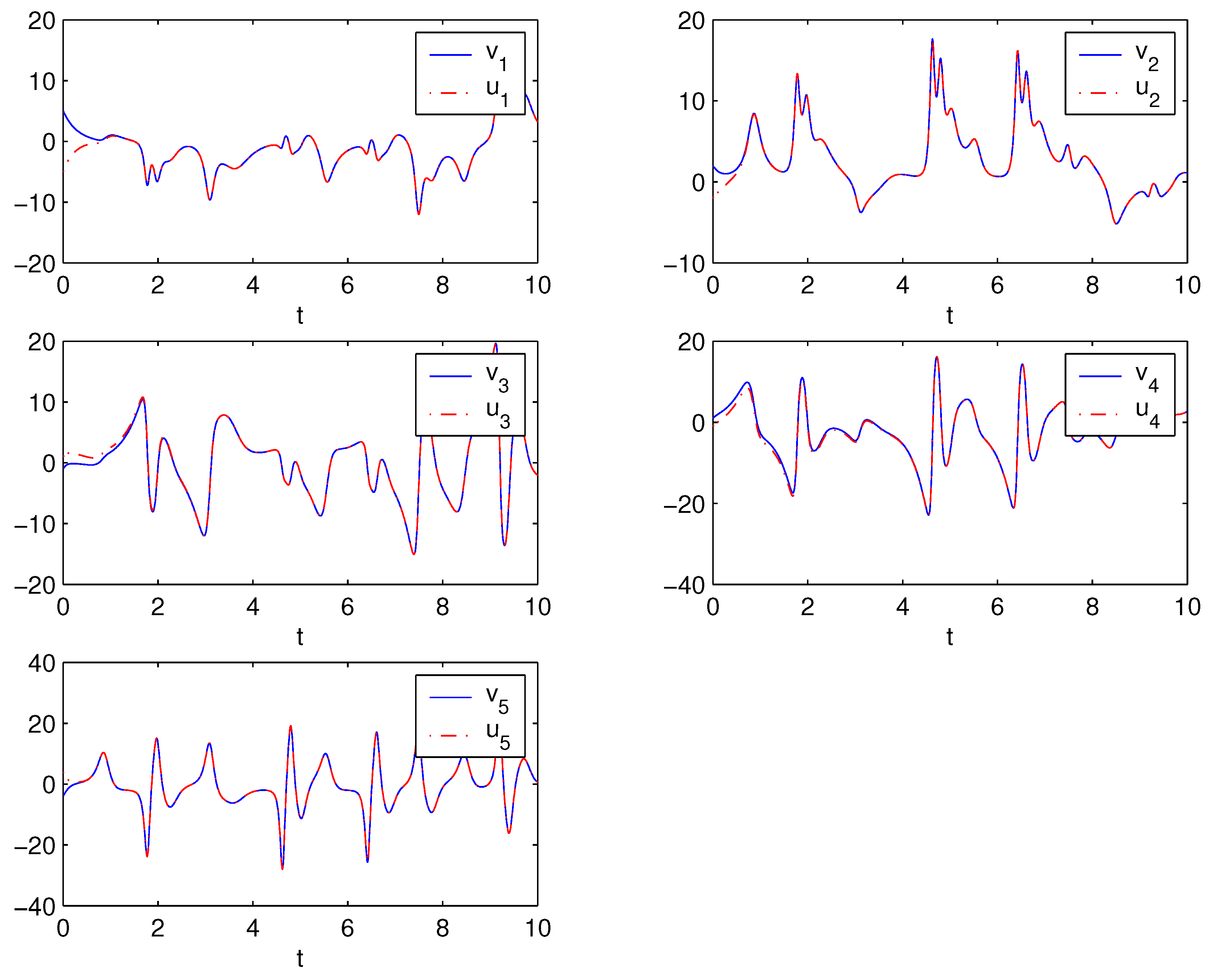
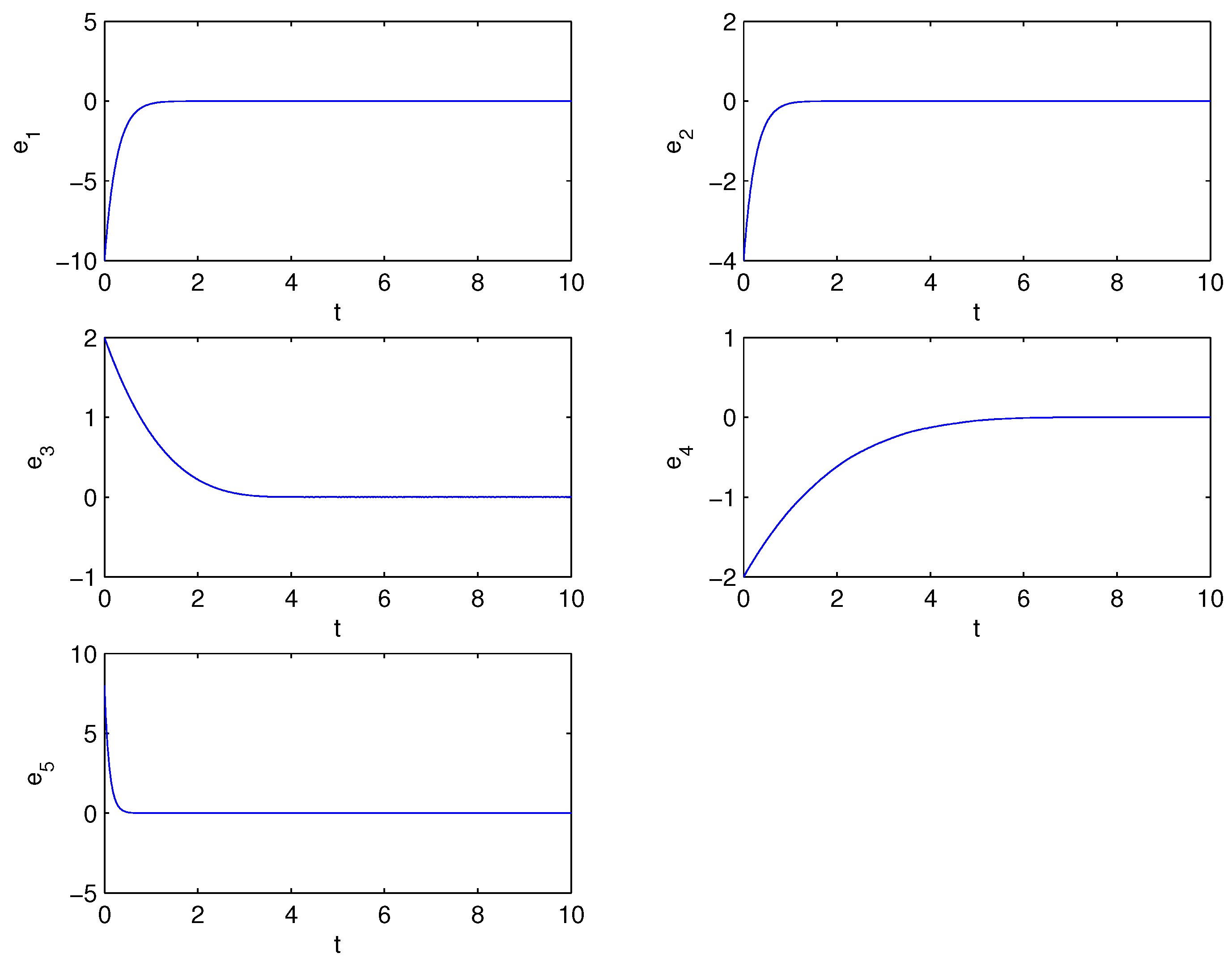
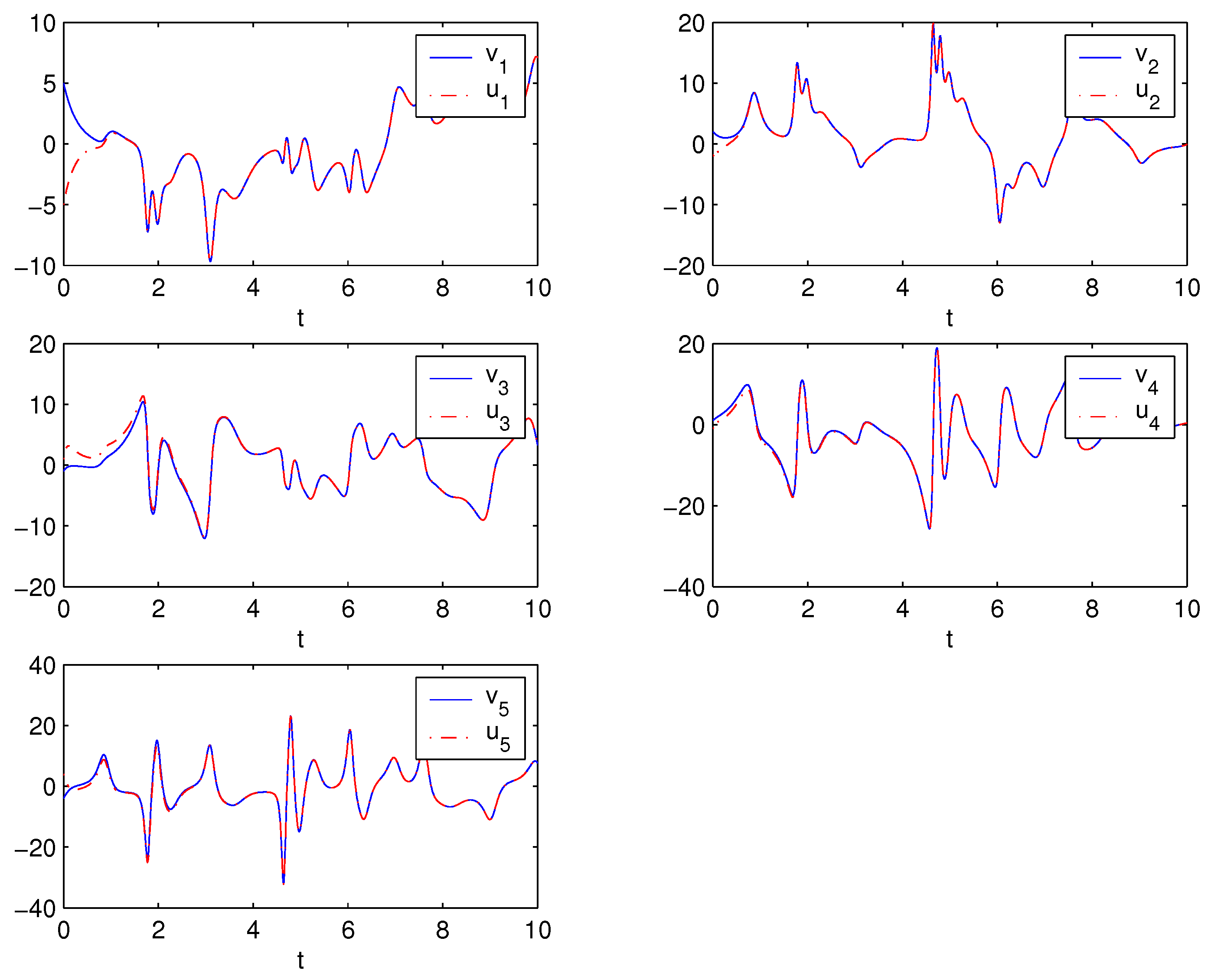
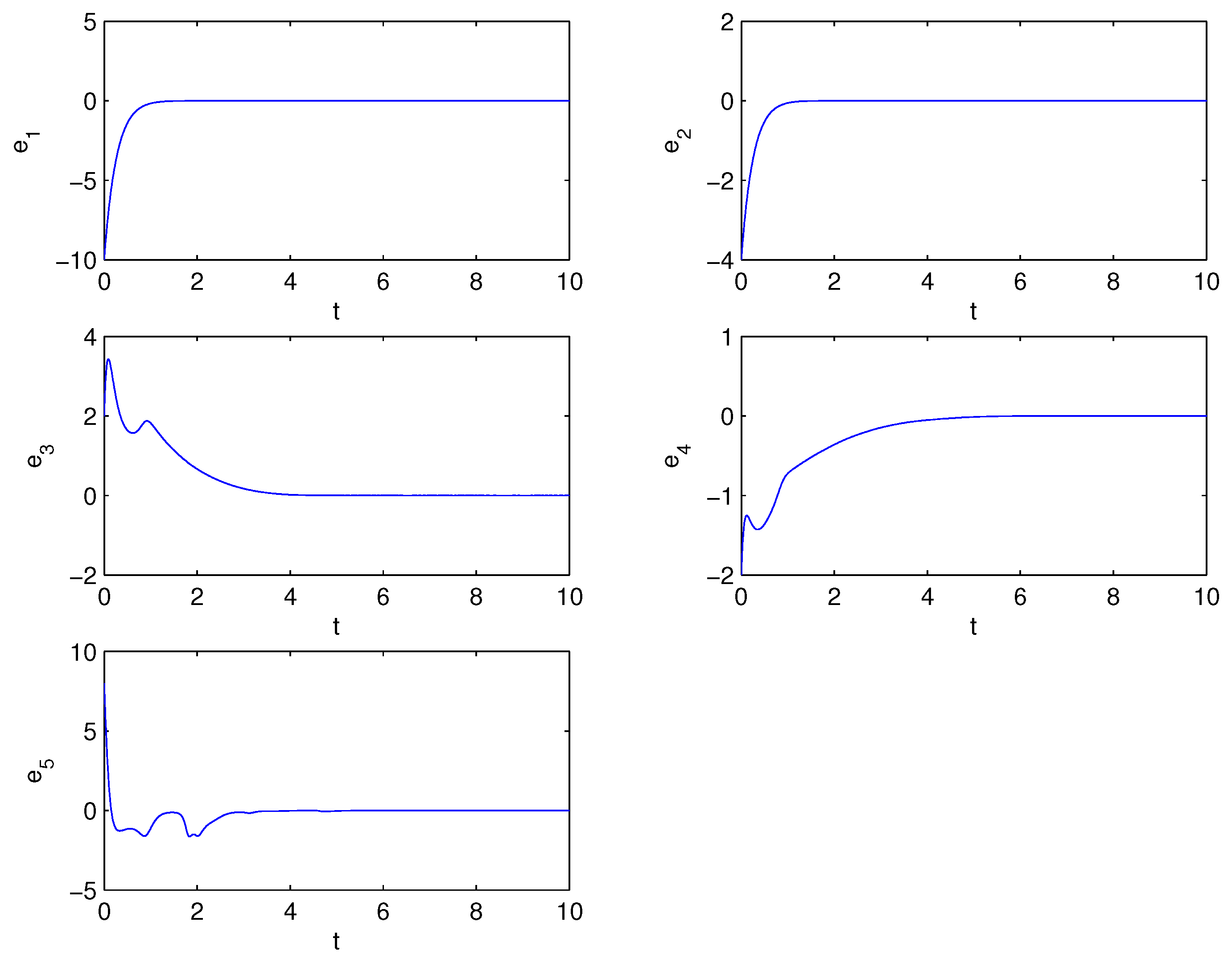
4. Numerical Simulations

In this section, two numerical examples are presented to illustrate the theoretical analysis. In the following numerical simulations the fourth-order Runge-kutta method is employed with time step size 0.001. The system parameters are selected as $a=3.5,b=0.6,c=3,d=2,$ and $h=9$, so that the complex nonlinear hyperchaotic system in Equation (1) exhibits hyperchaotic behavior. The initial conditions of the drive system and response system are always adopted as $\left(x\right(0),y(0),z(0\left)\right)=(5+2i,-1+i,-4)$ and $(x^{\prime }\left(0\right),y^{\prime }\left(0\right),z^{\prime }\left(0\right))=(-5-2i,1-i,4)$ respectively.

Example 1. Consider strategy 1 with the controllers given by Equation (11). We choose $L_1=3,L_2=3$ and $k=7/9$, Figure 1 and Figure 2 show the results of numerical simulation. From Figure 1, we can see that the states of the drive system from Equation (6) and the response system from Equation (7) quickly synchronize. Figure 2 shows the state errors $e_1,e_2,e_3,e_4,e_5$ are rapidly stabilize at zero. So the system given by Equations (6) and (7) achieves finite-time synchronization.

Figure 1. The states of the drive system in Equation (6) and the response system in Equation (7) with controllers given by Equation (11).

Figure 1. The states of the drive system in Equation (6) and the response system in Equation (7) with controllers given by Equation (11).

Figure 2. The time response of error states with controllers as in Equation (11).

Figure 2. The time response of error states with controllers as in Equation (11).

Example 2. Consider strategy 2 with the controllers given in Equation (16). We choose $L_3=3,L_4=3$ and $k=7/9$, Figure 3 and Figure 4 show that systems in Equations (6) and (7) achieve finite-time synchronization. From Figure 2 and Figure 4, we can see the synchronized time of error dynamical system in Figure 4 is longer than that in Figure 2.

Figure 3. The states of the drive system in Equation (6) and the response system in Equation (7) with controllers given by Equation (16).

Figure 3. The states of the drive system in Equation (6) and the response system in Equation (7) with controllers given by Equation (16).

Figure 4. The time response of error states with controllers as in Equation (16).

Figure 4. The time response of error states with controllers as in Equation (16).

5. Conclusions

When applying complex-variable systems in communications, the complex variables double the number of variables and can increase the content and security of the transmitted information. In this paper, a novel hyperchaotic complex-variable system which generates 2-, 3- and 4-scroll attractors has been considered and the fast synchronization problem of such a system has been investigated. Based on the finite-time stability theory, two kinds of simple and effective controllers for the novel hyperchaotic complex-variable system have been proposed to guarantee the global exponential stability of the resulting error systems. Finally, two numerical examples have been provided to illustrate the effectiveness of the theoretical analysis.

References

1. Rössler, O.E. An equation for hyperchaos. Phys. Lett. A 1979, 71, 155–157. [Google Scholar] [CrossRef]
2. Matsumoto, T.; Chua, L.O.; Kobayashi, K. Hyperchaos: Laboratory experiment and numerical confirmation. IEEE Trans. Circuits Syst. 1986, 33, 1143–1149. [Google Scholar] [CrossRef]
3. Grassi, G.; Mascolo, S. A system theory approach for designing cryptosystems based on hyperchaos. IEEE Trans. Circuits Syst. I 1999, 46, 1135–1138. [Google Scholar] [CrossRef]
4. Yin, H.; Chen, Z.; Yuan, Z. A blind watermarking algorithm based on hyperchaos and coset by quantizing wavelet transform coefficients. Int. J. Innov. Comput. Inf. Control 2007, 3, 1635–1643. [Google Scholar]
5. Zhu, C.X. A novel image encryption scheme based on improved hyperchaotic sequences. Opt. Commun. 2012, 285, 29–37. [Google Scholar] [CrossRef]
6. Fowler, A.C.; Gibbon, J.D.; McGuinness, M.J. The complex Lorenz equations. Physica D 1982, 4, 139–163. [Google Scholar] [CrossRef]
7. Ning, C.Z.; Haken, H. Detuned lasers and the complex Lorenz equations: Subcritical and supercritical Hopf bifurcations. Phys. Rev. A 1990, 41, 3826–3837. [Google Scholar] [CrossRef] [PubMed]
8. Gibbon, J.D.; McGuinness, M.J. The real and complex Lorenz equations in rotating fluids and lasers. Physica D 1983, 5, 108–122. [Google Scholar] [CrossRef]
9. Mahmoud, G.M.; Bountis, T.; Mahmoud, E.E. Active control and global synchronization of the complex Chen and Lü systems. Int. J. Bifurc. Chaos 2007, 17, 4295–4308. [Google Scholar] [CrossRef]
10. Mahmoud, G.M.; Bountis, T.; Al-Kashif, M.A.; Aly, S.A. Dynamical properties and synchronization of complex non-linear equations for detuned lasers. Dyn. Syst. 2009, 24, 63–79. [Google Scholar] [CrossRef]
11. Mahmoud, G.M.; Ahmed, M.E.; Sabor, N. On autonomous and nonautonomous modified hyperchaotic complex Lü systems. Int. J. Bifurc. Chaos 2011, 21, 1913–1926. [Google Scholar] [CrossRef]
12. Mahmoud, G.M.; Ahmed, M.E. A hyperchaotic complex system generating two-, three-, and four-scroll attractors. J. Vib. Control 2012, 18, 841–849. [Google Scholar] [CrossRef]
13. Chen, G.; Dong, X. From Chaos to Order: Methodologies, Perspectives and Applications; World Scientific: Singapore, Singapore, 1998. [Google Scholar]
14. Liao, T.; Huang, N. An observer-based approach for chaotic synchronization with applications to secure communications. IEEE Trans. Circuits Syst. I 1999, 46, 1144–1150. [Google Scholar] [CrossRef]
15. Boccaletti, S.; Grebogi, C.; Lai, Y.C.; Mancini, H.; Maza, D. The control of chaos: Theory and applications. Phys. Rep. 2000, 329, 103–197. [Google Scholar] [CrossRef]
16. Boccaletti, S.; Kurths, J.; Osipov, G.; Valladares, D.L.; Zhou, C.S. The synchronization of chaotic systems. Phys. Rep. 2002, 366, 1–101. [Google Scholar] [CrossRef]
17. Hu, M.; Yang, Y.; Xu, Z.; Guo, L. Hybrid projective synchronization in a chaotic complex nonlinear system. Math. Comput. Simul. 2008, 79, 449–457. [Google Scholar] [CrossRef]
18. Liu, S.; Liu, P. Adaptive anti-synchronization of chaotic complex nonlinear systems with unknown parameters. Nonlinear Anal. RWA 2011, 12, 3046–3055. [Google Scholar] [CrossRef]
19. Mahmoud, G.M.; Mahmoud, E.E.; Arafa, A.A. On projective synchronization of hyperchaotic complex nonlinear systems based on passive theory for secure communications. Phys. Scr. 2013, 87, 055002. [Google Scholar] [CrossRef]
20. Liu, P.; Liu, S. Robust adaptive full state hybrid synchronization of chaotic complex systems with unknown parameters and external disturbances. Nonlinear Dyn. 2012, 70, 585–599. [Google Scholar] [CrossRef]
21. Haimo, V.T. Finite time controllers. SIAM J. Control Optim. 1986, 24, 760–770. [Google Scholar] [CrossRef]
22. Vincent, U.E.; Guo, R. Finite-time synchronization for a class of chaotic and hyperchaotic systems via adaptive feedback controller. Phys. Lett. A 2011, 375, 2322–2326. [Google Scholar] [CrossRef]
23. Bhat, S.P.; Bernstein, D.S. Finite-time stability of continuous autonomous systems. SIAM J. Control Optim. 2000, 38, 751–766. [Google Scholar] [CrossRef]
24. Huang, X.Q.; Lin, W.; Yang, B. Global finite-time stabilization of a class of uncertain nonlinear systems. Automatica 2005, 41, 881–888. [Google Scholar] [CrossRef]