Efficiently Measuring Complexity on the Basis of Real-World Data

Abstract

Permutation entropy, introduced by Bandt and Pompe, is a conceptually simple and well-interpretable measure of time series complexity. In this paper, we propose efficient methods for computing it and related ordinal-patterns-based characteristics. The methods are based on precomputing values of successive ordinal patterns of order d, considering the fact that they are “overlapped” in d points, and on precomputing successive values of the permutation entropy related to “overlapping” successive time-windows. The proposed methods allow for measurement of the complexity of very large datasets in real-time.

1. Introduction

1.1. Motivation

Measuring the complexity of a system by observed time series is an important problem in different fields of research. One faces the problem, for instance, of distinguishing between different brain states on the base of EEG data. The complexity of a dynamical system can be measured by the well-motivated Kolmogorov-Sinai (KS) entropy [1], by the Lyapunov exponent, or by the correlation dimension [2], but it is often not easy to estimate these and similar quantities from finite real-world data.

In order to quantify complexity on the base of real-world data, Bandt and Pompe have introduced permutation entropy [3]. It is based on the distributions of ordinal patterns, which describe order relations between the values of a time series. On the one hand, permutation entropy is strongly related to KS entropy. It coincides with KS entropy for piecewise strictly monotone interval maps [4] and is not less than KS entropy for many dynamical systems [5,6,7] (see also [8,9] for some new results in this direction and [10] for the discussion of two approaches to the permutation entropy with respect to KS entropy). On the other hand, permutation entropy is estimated by empirical permutation entropy, which is conceptually simple and algorithmically fast [3,11]. Empirical permutation entropy also provides robustness with respect to noise [3,12]. An important practical aspect of empirical permutation entropy is that one can compare by it complexities of different time series of a fixed length in a well-interpretable, standardized and simple way.

Justified theoretically and simple conceptually, empirical permutation entropy and different ordinal-patterns-based characteristics have been applied in various fields for analyzing real-world data: for detecting and visualizing EEG changes related to epileptic seizures (e.g., [13,14,15,16]), for distinguishing brain states related to anesthesia [17,18], for discriminating sleep stages in EEG data [19], for analyzing and classifying heart rate variability data [20,21,22,23], and for financial, physical and statistical time series analysis (see [10,12] for a review of applications).

Motivated by the good properties and many applications of empirical permutation entropy, we propose in this paper an efficient method of computing it and ordinal patterns faster than in [11], which allows for processing very large data sets in real-time. An efficient computation of ordinal patterns provides a fast calculation of not only empirical permutation entropy, but of many ordinal-patterns-based characteristics, such as, for example, the ordinal distributions itself [24] and derived measures [25], or transcripts, introduced in [26]. The concept behind an efficient method is to use precomputed tables of successive values instead of computing ordinal patterns and the empirical permutation entropy in each time point. It is possible to precompute such successive values, because ordinal patterns “overlap” and, in fact, have some common information. Since successive values of the empirical permutation entropy are computed for successive overlapping time-windows, the possible “successive” entropies can also be precomputed.

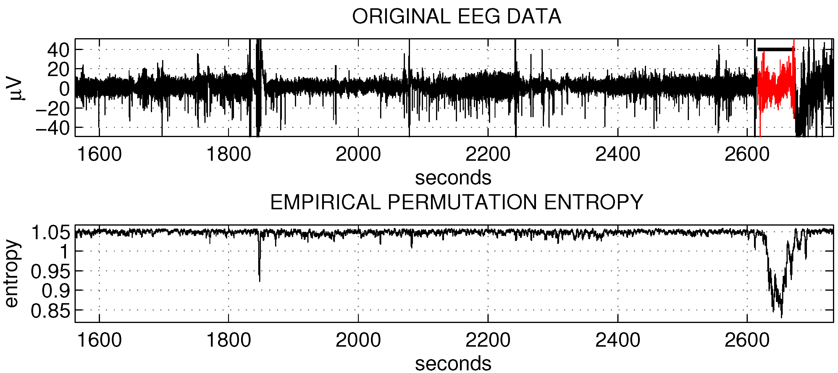
Figure 1. The empirical permutation entropy reflects changes of the epileptic EEG data.

Figure 1. The empirical permutation entropy reflects changes of the epileptic EEG data.

To motivate the method, let us give an example of processing epileptic EEG data by the empirical permutation entropy (data from The European Epilepsy Database [27]). Figure 1 illustrates how the empirical permutation entropy (bottom plot) reflects the epileptic seizure (marked in red and with a “head”) in one-channel EEG data (upper plot). The processing of the depicted 20 min of EEG data, recorded at a sampling rate of 256 Hz, takes about 1 second in MATLAB R2012b.

In Section 2 we recall some notions from ordinal patterns analysis and consider how to compute ordinal patterns (by the method introduced in [11]) and how to compute the empirical permutation entropy from the distributions of ordinal patterns. More efficient methods for computing ordinal patterns and the empirical permutation entropy are introduced in Section 3 and Section 4, correspondingly. In Section 5 we adapt the method to time series with a high frequency of occurrence of equal values. It is reasonable to take into account these equalities for data digitized with a low resolution, for example, for heart rate variability data as they are considered in [23]. Finally, we present the comparison between two known methods of computing the empirical permutation entropy and the proposed method in Section 6.

2. Computing Ordinal Patterns and the Empirical Permutation Entropy

In this section we recall how to compute ordinal patterns by the method introduced in [11] and how to compute the empirical permutation entropy from the obtained distributions of ordinal patterns.

2.1. Ordinal Patterns

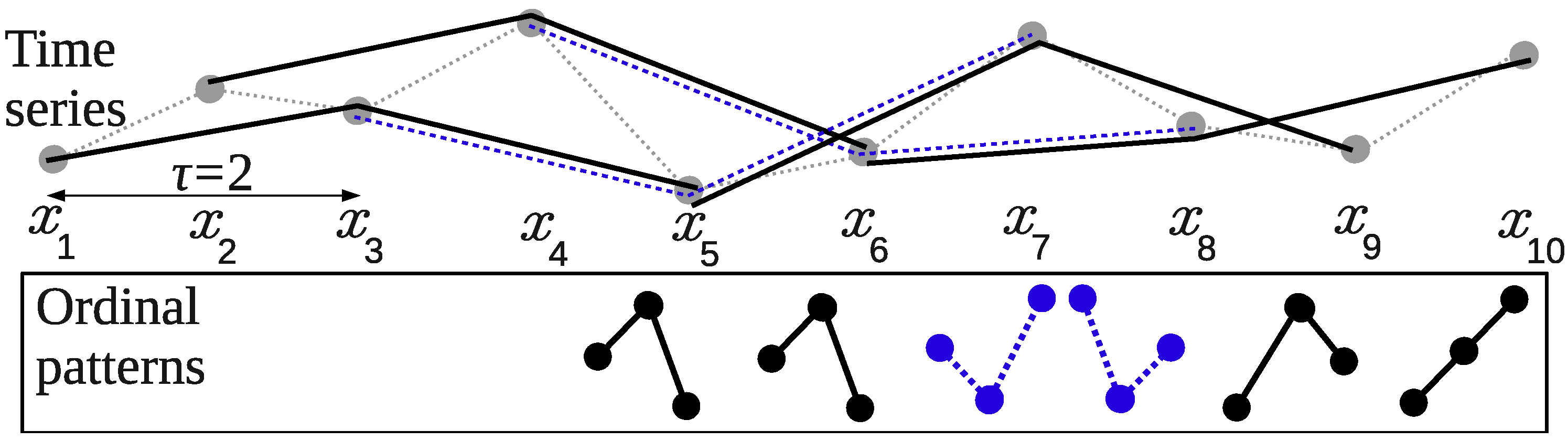
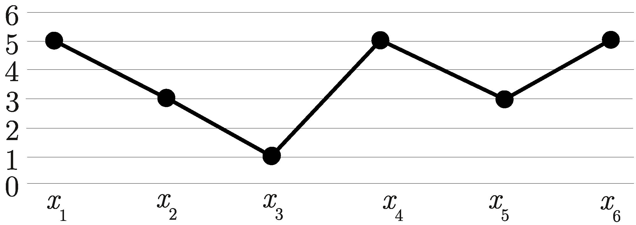
Let us start from an example of computing ordinal patterns (see Figure 2). We consider a part of a time series, consisting of 10 points, we fix a delay $\tau =2$, which indicates a distance between points in ordinal patterns, and an order $d=2$, meaning ordinal patterns contain $(d+1)=3$ points.

Figure 2. The ordinal patterns of order $d=2$.

Figure 2. The ordinal patterns of order $d=2$.

One can see that the blue ordinal patterns (in dashed line) “overlap” the previous black ordinal patterns in $d=2$ points, and then the black ordinal patterns “overlap” the previous blue ordinal patterns in $d=2$ points. This “overlapping” allows to use all information about order relations between points that can be obtained from a time series. By the same reason the ordinal patterns are computed starting from the point $x_1$ (the first, the third and the fifth ones) and then with a shift 1, starting from the point $x_2$ (the second, the fourth and the sixth ones). In the general case, ordinal patterns are computed starting from all initial times $1,\dots ,\tau$.

2.1.1. Number Representation

In order to obtain the distribution of ordinal patterns, we assign numbers to each type of ordinal patterns. We consider here the enumeration of ordinal patterns introduced in [11], because it allows to compute them relatively fast. Originally, ordinal patterns of order d were defined as permutations of the set $\{0,1,\dots ,d\}$ (see [3,11]). However, we define them here in the following way since that provides a simple enumeration of them (we refer for details to [11]).

Definition 1. 

The delay vector $(x_t,x_{t-\tau },\dots ,x_{t-d\tau })$ is said to have the ordinal pattern $(i_1^{\tau }(t),i_2^{\tau }(t),\dots ,i_d^{\tau }(t))$ of order d and delay τ if $i_l^{\tau }(t)$ for $l=1,2,\dots ,d$ is given by

$$i_l^{\tau }(t)=\#\{r\in \{0,1,\dots ,l-1\}\mid x_{t-l\tau }\ge x_{t-r\tau }\}$$

(1)

Simply speaking, each $i_l^{\tau }(t)$ codes how many points from $(x_t,x_{t-\tau },\dots ,x_{t-(l-1)\tau })$ are not larger than $x_{t-l\tau }$. Note that we assume here occurrence of equal values in a time series quite rare. Indeed, the relation “equal to” is combined with the relation “greater than” in Definition 1. Regarding the time series with a high frequency of occurrence of equal values, we discuss modified ordinal patterns with considering equality in Section 5.

There are $(d+1)!$ ordinal patterns of order d, and one assigns to each of them a number from $\{0,1,\dots ,(d+1)!-1\}$ in a one-to-one way by

$$n_d^{\tau }(t)=n_d^{\tau }((i_1^{\tau }(t),i_2^{\tau }(t),\dots ,i_d^{\tau }(t)))=\sum _{l=1}^d{i}_l^{\tau }(t)\frac{(d+1)!}{(l+1)!}$$

(2)

For example, all ordinal patterns of order $d=2$ in their number representation are given in Table 1. Note that the ordinal patterns with the numbers $(d+1)(k-1),\dots ,(d+1)k-1$ for each $k=1,2,\dots ,d!$ have the same relations between the last d points, because they have the same $(i_1,i_2,\dots ,i_{d-1})$ but a different $i_d$. For instance, the ordinal patterns $0,1,2$ (as well as the ordinal patterns $3,4,5$) have the same relation between the last $d=2$ points since they have the same $i_1$ and a different $i_2$ (see Table 1). We will use this property in Subsection 3.3.

Table 1. The ordinal patterns of order $d=2$.

Ordinal pattern
$(i_1,i_2)$	(0,0)	(0,1)	(0,2)	(1,0)	(1,1)	(1,1)
$n_2(i_1,i_2)=3i_1+i_2$	0	1	2	3	4	5

Table 1. The ordinal patterns of order $d=2$.

Ordinal pattern
$(i_1,i_2)$	(0,0)	(0,1)	(0,2)	(1,0)	(1,1)	(1,1)
$n_2(i_1,i_2)=3i_1+i_2$	0	1	2	3	4	5

2.1.2. Successive Ordinal Patterns

Due to the “overlapping” between ordinal patterns one easily obtains the successive ordinal pattern $(i_1^{\tau }(t+\tau ),i_2^{\tau }(t+\tau ),\dots ,i_d^{\tau }(t+\tau ))$ from the previous one $(i_1^{\tau }(t),i_2^{\tau }(t),\dots ,i_d^{\tau }(t))$ by

$$i_{l+1}^{\tau }(t+\tau )=\left\{\begin{array}{cc}{i}_l^{\tau }(t)\hfill & \text{if}{x}_{t-l\tau }<x_{t+\tau }\hfill \\ i_l^{\tau }(t)+1\hfill & \text{otherwise}\hfill \end{array}\right.$$

(3)

($i_1^{\tau }(t+\tau )$ is determined by Equation (1)). According to Equation (3) one needs only d comparisons and at most d incrementation operations to obtain the successive ordinal pattern when the current ordinal pattern is given [11]. When counting ordinal patterns in their number representation (2), which is clearly more convenient than in the representation provided by Equation (1), one needs d multiplications more.

2.2. The Empirical Permutation Entropy

In order to reflect complexity changes in a time series in the course of time, the empirical permutation entropy is usually computed in sliding time-windows of a fixed size.

Definition 2. 

By the empirical permutation entropy of order d and of delay τ of a time-window $(x_t,x_{t-1},\dots ,x_{t-M-d\tau +1})$ at time t one understands the quantity

$$\begin{array}{c}\hfill h_d^{\tau }(t)=-\sum _{j=0}^{(d+1)!-1}\frac{q_j}{M}ln\frac{q_j}{M}=lnM-\frac{1}{M}\sum _{j=0}^{(d+1)!-1}{q}_{j}ln{q}_j,\text{where}\\ \hfill q_j=\#\{k\in \{t,t-1,\dots ,t-M+1\}\mid (x_k,x_{k-\tau },\dots ,x_{k-d\tau })\text{has}\text{the}\text{ordinal}\text{pattern}j\}\end{array}$$

(4)

(with $0ln0:=0$).

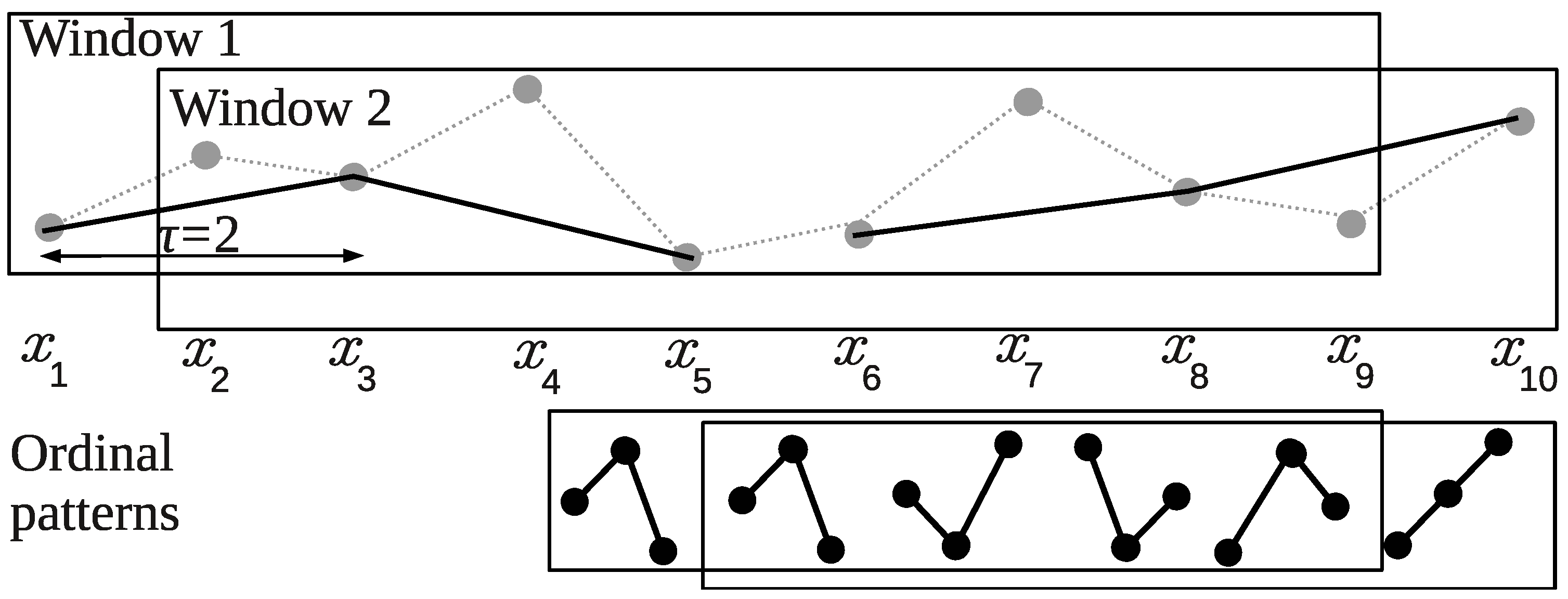
Note that the window size M is defined as the number of ordinal patterns in the window. Let us give an example of computing the empirical permutation entropy in the two sliding windows $(x_1,x_2,\dots ,x_9)$ and $(x_2,x_3,\dots ,x_{10})$, containing $M=5$ ordinal patterns of order $d=2$ with a delay $\tau =2$ (see Figure 3).

Figure 3. Computing the empirical permutation entropy in a sliding window.

Figure 3. Computing the empirical permutation entropy in a sliding window.

The windows overlap in 8 points and in 4 ordinal patterns. There are $q_0=0,q_1=1,q_2=1,q_3=1,q_4=2,q_5=0$ and $q_0=1,q_1=1,q_2=1,q_3=1,q_4=1,q_5=0$ ordinal patterns in Window 1 and in Window 2, correspondingly (see Table 1 for determining their types). Then the empirical permutation entropy at time $t=9$ and $t=10$ is computed by Equation (4) as

$$\begin{array}{c}\hfill h_2^2(9)=ln5-\frac{1}{5}(1ln1+1ln1+1ln1+2ln2)=1.3322\\ \hfill h_2^2(10)=ln5-\frac{1}{5}(1ln1+1ln1+1ln1+1ln1+1ln1)=1.6094\end{array}$$

3. Efficiently Computing Ordinal Patterns

In this section, we precompute successive ordinal patterns for each ordinal pattern. Using these values allows to compute ordinal patterns as numbers about two times faster than by EquationS (2) and (3). This is important for the fast calculation of ordinal-patterns-based characteristics, in particular, the empirical permutation entropy.

For simplicity, we use here the number representation of ordinal patterns provided by Equation (2), but, in fact, the type of number representation is not substantial for the method, as we discuss in Subsection 3.3.

3.1. Precomputed Successive Ordinal Patterns

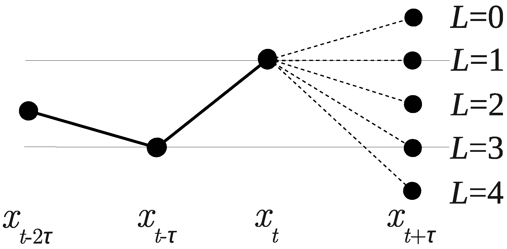
Given the ordinal pattern $n_d^{\tau }(t)$ there are $(d+1)$ possible successive ordinal patterns $n_d^{\tau }(t+\tau )$ since there are $(d+1)$ positions of the point $x_{t+\tau }$ relative to the points from $(x_t,x_{t-\tau },\dots ,x_{t-(d-1)\tau })$. Ordinal patterns of order $d=2$ and their successive ones are presented in Table 2. For example, for the ordinal pattern 0 there are three possible positions $l=0,1,2$ of the next point and three possible successive ordinal patterns $0,3,4$, respectively.

Table 2. The successive ordinal patterns $n_2^{\tau }(t+\tau )$ given $n_2^{\tau }(t)$.

Current ordinal pattern
Successive ordinal pattern	0			1
	3			2
	4			5

Table 2. The successive ordinal patterns $n_2^{\tau }(t+\tau )$ given $n_2^{\tau }(t)$.

Current ordinal pattern
Successive ordinal pattern	0			1
	3			2
	4			5

Let us denote the function determining successive ordinal patterns from a given one and from the position of the next value by ${\varphi }_d$:

$$n_d^{\tau }(t+\tau )={\varphi }_d(n_d^{\tau }(t),l)$$

(5)

where l indicates how many points from $(x_t,x_{t-\tau },\dots ,x_{t-(d-1)\tau })$ are greater than or equal to $x_{t+\tau }$, i.e.,

$$l=\#\{r\in \{0,1,\dots ,d-1\}\mid x_{t-r\tau }\ge x_{t+\tau }\}$$

(6)

For example, the values of the function ${\varphi }_2$, determining the successive ordinal pattern $n_2^{\tau }(t+\tau )$ from the given ordinal pattern $n_2^{\tau }(t)$, are presented in Table 3. One could determine the position l also as how many points from $(x_t,x_{t-\tau },\dots ,x_{t-(d-1)\tau })$ are less than or equal to $x_{t+\tau }$. The way of determining l is not substantial since it changes only the representation of the precomputed table.

Table 3. The successive ordinal patterns $n_2^{\tau }(t+\tau )={\varphi }_d(n_2^{\tau }(t),l)$.

	$n_2^{\tau }(t)$
position $l$	0	1	2	3	4	5
0	0			1
1	3			2
2	4			5

Table 3. The successive ordinal patterns $n_2^{\tau }(t+\tau )={\varphi }_d(n_2^{\tau }(t),l)$.

	$n_2^{\tau }(t)$
position $l$	0	1	2	3	4	5
0	0			1
1	3			2
2	4			5

3.2. How can the Precomputed Table be Obtained?

One obtains the entries of the table by determining for each ordinal pattern of order d all possible successive ordinal patterns in dependence on the position $l=0,1,\dots ,d$ of the next point. When using the number representation (2), one obtains the successive ordinal patterns $(i_1^{\tau }(t+\tau ),i_2^{\tau }(t+\tau ),\dots ,i_d^{\tau }(t+\tau ))$ from the given ordinal pattern $(i_1^{\tau }(t),i_2^{\tau }(t),\dots ,i_d^{\tau }(t))$ for all $l=0,1,\dots ,d$ by Equation (3). Then the entries of the table are obtained by Equation (2). The precomputed tables of successive ordinal patterns of the orders $d=1,2,\dots ,8$ are given in the supplementary files “table1.mat”,...,“table8.mat”.

3.3. Size of the Precomputed Table

In order to efficiently compute ordinal patterns by Equation (5), one has to store $(d+1)$ values ${\varphi }_d(n_d^{\tau },l)$ for each of the $(d+1)!$ ordinal patterns $n_d^{\tau }$, i.e., $(d+1)!(d+1)$ values in total. This is usually not a very large size since in many situations the orders $d=3,\dots ,7$ are recommended for applications [3].

When using the enumeration (2) one can reduce the size of the table. Indeed, the ordinal patterns with the numbers $(d+1)(k-1),\dots ,(d+1)k-1$ for each $k=1,2,\dots ,d!$ have the same successive ordinal patterns, because they describe the same relation between the last d points (Subsection 2.1). For example, the ordinal patterns $0,1,2$ as well as the ordinal patterns $3,4,5$ have the same successive ordinal patterns: ${\varphi }_d(0,l)={\varphi }_d(1,l)={\varphi }_d(2,l)$ and ${\varphi }_d(3,l)={\varphi }_d(4,l)={\varphi }_d(5,l)$ (see Table 2).

Note that one can use enumerations of ordinal patterns different from (2) since only the correct correspondence between successive ordinal patterns is needed to efficiently compute them by Equation (5).

3.4. Efficiency of the Method

When efficiently determining the number $n_d^{\tau }(t+\tau )$ from $n_d^{\tau }(t)$ by Equation (5), one calculates only l by Equation (6). This is almost twice faster than calculating $n_d^{\tau }(t+\tau )$ by Equation (2), involving calculation (3) (see Table 4).

Table 4. Efficiency of computing the ordinal pattern $n_d^{\tau }(t+\tau )$ from $n_d^{\tau }(t)$.

Computation of $n_d^{\tau }(t+\tau )$	+	Incrementation	*	$<>$	The total number of operations
by Equation (2), involving Equation (3)	d	≤d	$d-1$	d	≤$4d-1$
by Equation (5)	0	≤d	0	d	≤$2d$

Table 4. Efficiency of computing the ordinal pattern $n_d^{\tau }(t+\tau )$ from $n_d^{\tau }(t)$.

Computation of $n_d^{\tau }(t+\tau )$	+	Incrementation	*	$<>$	The total number of operations
by Equation (2), involving Equation (3)	d	≤d	$d-1$	d	≤$4d-1$
by Equation (5)	0	≤d	0	d	≤$2d$

4. Efficiently Computing the Empirical Permutation Entropy

In this section, we consider the empirical permutation entropy, computed in sliding windows of a size M with maximal overlapping, i.e., the first point of the successive window is the second point of the previous one. The case with non-maximal overlapping is discussed in Subsection 4.3.

4.1. Precomputed Values

The successive windows $(x_{t-1},x_{t-2},\dots ,x_{t-M-d\tau })$ and $(x_t,x_{t-1}\dots ,x_{t-M-d\tau +1})$ differ in the points $x_t$ and $x_{t-M-d\tau }$, therefore the ordinal distributions in the windows differ in the frequencies of occurrence of the ordinal patterns $n_d^{\tau }(t)$ and $n_d^{\tau }(t-M)$. In order to obtain the ordinal distribution of the successive window given the current one, one needs to substitute the frequency of the “outcoming” ordinal pattern $q_{n_d^{\tau }(t)}$ by $(q_{n_d^{\tau }(t)}-1)$ and the frequency of the “incoming” ordinal pattern $q_{n_d^{\tau }(t)}$ by $(q_{n_d^{\tau }(t)}+1)$:

$$\begin{array}{c}\hfill q_{n_d^{\tau }(t-M)}ln{q}_{n_d^{\tau }(t-M)}⟶(q_{n_d^{\tau }(t-M)}-1)ln(q_{n_d^{\tau }(t-M)}-1)\\ \hfill q_{n_d^{\tau }(t)}ln{q}_{n_d^{\tau }(t)}⟶(q_{n_d^{\tau }(t)}+1)ln(q_{n_d^{\tau }(t)}+1)\end{array}$$

Then the empirical permutation entropy $h_d^{\tau }(t)$ given $h_d^{\tau }(t-1)$ is computed by

$$\begin{array}{c}\hfill h_d^{\tau }(t)=h_d^{\tau }(t-1)+g(q_{n_d^{\tau }(t)}+1)-g(q_{n_d^{\tau }(t-M)}),\text{where}\end{array}$$

(7)

$$\begin{array}{c}\hfill g(j)=\frac{1}{M}\left(jlnj-(j-1)ln(j-1)\right)\text{for}j=1,2,\dots ,M\\ \hfill q_{n_d^{\tau }(t)}=\#\{k\in \{t,t-1,\dots ,t-M+1\}\mid (x_k,x_{k-\tau },\dots ,x_{k-d\tau })\text{has}\text{the}\text{ordinal}\text{pattern}{n}_d^{\tau }(t)\}.\end{array}$$

(8)

If the “incoming” ordinal pattern coincides with the “outcoming” ordinal pattern, the ordinal distributions and the values of the empirical permutation entropy are the same for successive windows.

4.2. How can the Precomputed Table be Obtained: Size of the Precomputed Table

The precomputed table is obtained by computing (8) for all $j=1,2,\dots ,M$, where M is the size of a sliding window. We have used a window size of two seconds in the example in the Introduction, which implies the size $M=2·256=512$ of the precomputed table for a sampling rate of 256 Hz (see Figure 1).

4.3. Efficiency of the Method

Assuming that the distribution of ordinal patterns for the window $(x_{t-1},x_{t-2},\dots ,x_{t-M-d\tau })$ and $h_d^{\tau }(t-1)$ are known, we compare the computation of $h_d^{\tau }(t)$ by Equation (4) and by Equation (7) (see Table 5).

Table 5. Efficiency of computing the empirical permutation entropy $h_d^{\tau }(t)$.

Calculation	+	*	ln	The total number of operations
by Equation (4)	≤$(d+1)!-1$	$(d+1)!$	$(d+1)!$	≤$3(d+1)!-2$
by Equation (7)	2	0	0	2

Table 5. Efficiency of computing the empirical permutation entropy $h_d^{\tau }(t)$.

Calculation	+	*	ln	The total number of operations
by Equation (4)	≤$(d+1)!-1$	$(d+1)!$	$(d+1)!$	≤$3(d+1)!-2$
by Equation (7)	2	0	0	2

However, when using Equation (7) the empirical permutation entropy $h_d^{\tau }(t)$ for the first window is computed by Equation (4) since there is no precomputed value $h_d^{\tau }(t-1)$. There are also no precomputed numbers of ordinal patterns for the first τ ordinal patterns. Computing their numbers by Equation (2) takes at most $(4d-1)\tau$ operations (see Figure 5 for the scheme of the method).

In the case of non-maximal overlapping between windows, one can also compute the empirical permutation entropy by Equation (7), omitting “unnecessary” intermediate values $h_d^{\tau }(t)$. This is reasonable when the distance between the windows is not very large, and computing the empirical permutation entropy by Equation (4) implies more operations than by Equation (7). Roughly speaking, for a distance $D<\frac{3(d+1)!-2}{2}$ between successive windows computing the empirical permutation entropy for the whole time series with use of sliding windows by Equation (7) is faster than by Equation (4).

4.4. Round-off Error

Successively calculating the empirical permutation entropy by Equation (7) provides an accumulation of round-off errors resulting from finite computer precision. One performs two operations in Equation (7) at each of W time points, which bounds the error by $2W\psi$, where ψ is the machine precision and W is the length of a time series. For a relatively long time series one can recalculate the empirical permutation entropy by Equation (4) after some time, depending on the computer precision again, in order to avoid big accumulating errors and then continue calculations by Equation (7). For example, if ϵ is the maximal allowable error in computing the empirical permutation entropy, then one should recalculate the empirical permutation entropy by Equation (4) every $\frac{ϵ}{2\psi }$ points.

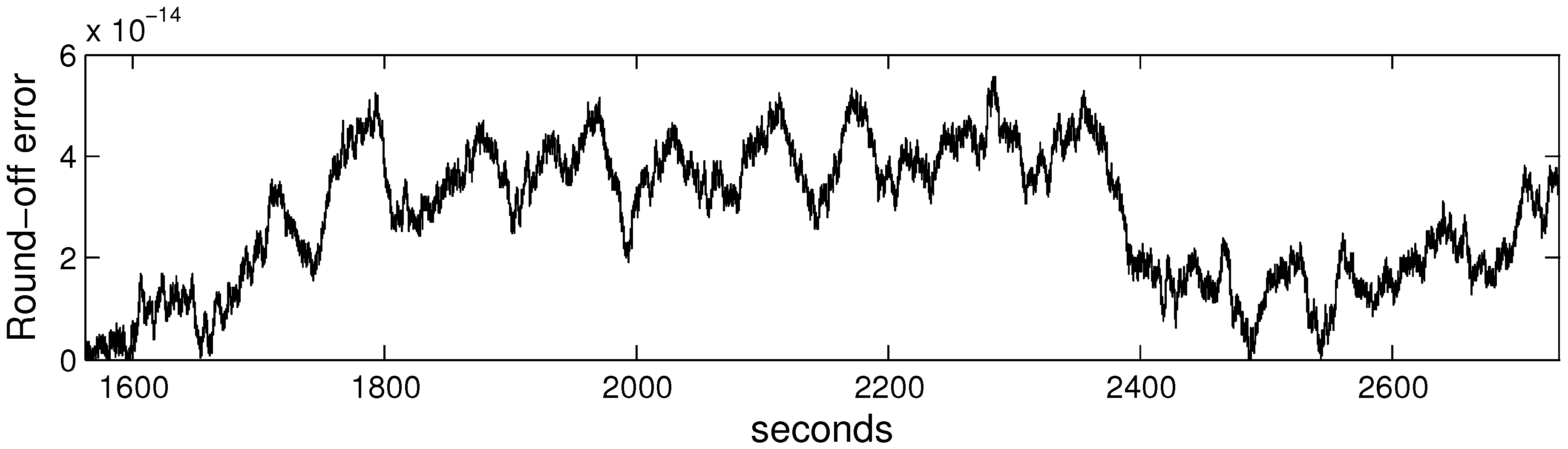
For illustration purposes we present the round-off error of the empirical permutation entropy obtained for the example shown in the Introduction in Figure 4. One can see that the error is very small in relation to the values of the empirical permutation entropy (compare with Figure 1).

Figure 4. Round-off error of the empirical permutation entropy computed in dependence on time.

Figure 4. Round-off error of the empirical permutation entropy computed in dependence on time.

4.5. Method Summary

We summarize the proposed method of the efficient computation of the empirical permutation entropy in the following scheme (see Figure 5). As above, the size of a sliding window is denoted by M, the order of ordinal patterns by d, the delay by τ and the length of a time series by W. The MATLAB code for computing the empirical permutation entropy is given in Appendix B.1.

Figure 5. Computational scheme of the method.

Figure 5. Computational scheme of the method.

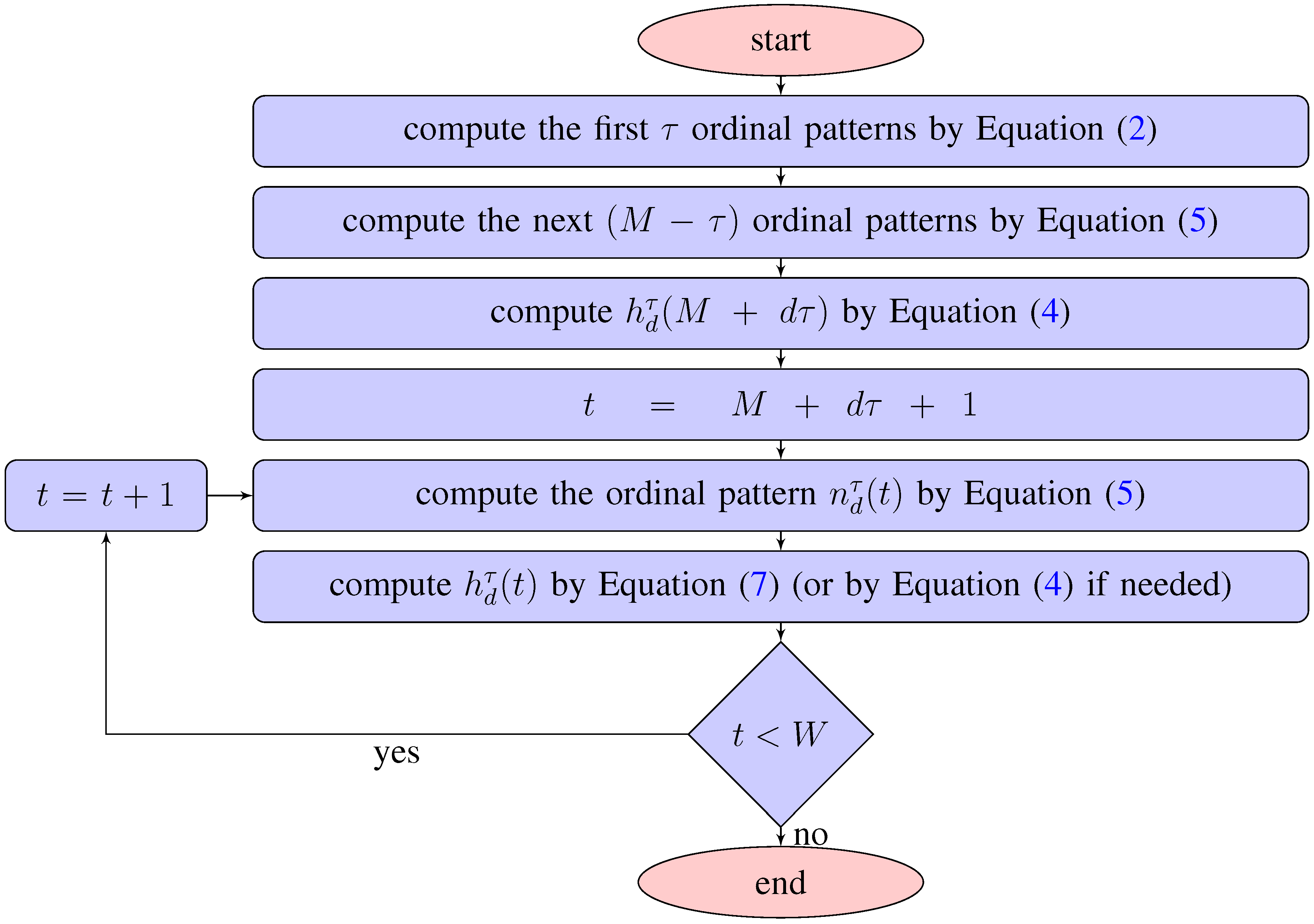
Note that according to the scheme the efficiency of the proposed method after computing $h_d^{\tau }(M+d\tau )$ by Equation (4) depends only on a length of a time series W and does not depend neither on the order d, the window size M nor on the delay τ.

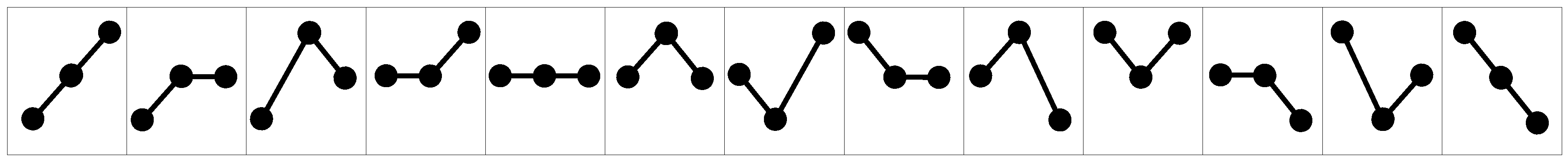
5. Efficiently Computing Modified Ordinal Patterns

This section is devoted to the efficient computation of modified ordinal patterns, which are adapted to the case of a time series with a high frequency of occurrence of equal values. In order to give an impression, we present all modified ordinal patterns of order $d=2$ in Figure 6. Modified ordinal patterns are efficiently computed by using the idea of precomputed successive values similarly as it is done in Section 3. In Subsection 5.1.2. we propose a possible variant of their enumeration, which is natural from the computational point of view and provides a “short” precomputed table (as in Subsection 3.3). However, the way of enumerating modified ordinal patterns is also not substantial for computing them efficiently.

Figure 6. The modified ordinal patterns of order $d=2$.

Figure 6. The modified ordinal patterns of order $d=2$.

5.1. Modified Ordinal Patterns

There are many ways to code modified ordinal patterns. We code them naturally by determining for the vector $(x_t,x_{t-\tau },\dots ,x_{t-d\tau })$ the position of each point $x_{t-l\tau }$ in relation to the points from the same vector. There are now three possibilities of the relation between two points: one point can be greater (less) than another one or equal to another one.

Let us indicate by $b_l^{\tau }(t)$, whether the point $x_{t-l\tau }$ is equal to any point from $(x_t,x_{t-\tau },\dots ,x_{t-(l-1)\tau })$:

$$b_l^{\tau }(t)=\left\{\begin{array}{cc}1\hfill & \text{if}{x}_{t-l\tau }=x_{t-j\tau }\text{for}\text{some}j\in \{0,1,\dots ,l-1\}\hfill \\ 0\hfill & \text{otherwise}\hfill \end{array}\right.$$

(9)

Then the position $I_l^{\tau }(t)$ of the point $x_{t-l\tau }$ in relation to the points from $(x_t,x_{t-\tau },\dots ,x_{t-(l-1)\tau })$ is calculated as

$$I_l^{\tau }(t)=b_l^{\tau }(t)+2\#\{r\in \{0,1,\dots ,l-1\}\mid x_{t-l\tau }>x_{t-r\tau },b_r^{\tau }(t)=0\}$$

(10)

In words, in order to determine the position of the point $x_{t-l\tau }$ in relation to the points $(x_t,x_{t-\tau },\dots ,x_{t-d\tau })$ one counts how many values among the points in $(x_t,x_{t-\tau },\dots ,x_{t-d\tau })$ are less than $x_{t-l\tau }$ and indicates whether the point $x_{t-l\tau }$ is equal to any other point from $(x_t,x_{t-\tau },\dots ,x_{t-d\tau })$.

Definition 3. 

A delay vector $(x_t,x_{t-\tau },\dots ,x_{t-d\tau })$ is said to have the modified ordinal pattern $(I_1^{\tau }(t),I_2^{\tau }(t),\dots ,I_d^{\tau }(t))$ of order d and delay τ if $I_l^{\tau }(t)$ for $l=1,2,\dots ,d$ is given by Equation (10).

Also note that the proposed coding of modified ordinal patterns is very concise because one stores all information about the relations between the points in one vector $(I_1^{\tau }(t),I_2^{\tau }(t),\dots ,I_d^{\tau }(t))$. Let us give an example of calculating the modified ordinal pattern of order $d=5$ and delay $\tau =1$ (see Figure 7). For instance, the point $x_1$ is equal to the points $x_4$ and $x_6$, i.e., $b_5^1(6)=1$, and it is greater than the two values $x_2=x_5$ and $x_3$, i.e., $I_5^1(6)=2·2+1=5$. One can easily check the position of the point $x_1$ when counting positions from the bottom up.

Figure 7. The modified ordinal pattern $(I_1^1(6),I_2^1(6),I_3^1(6),I_4^1(6),I_5^1(6))=(0,3,0,3,5)$.

Figure 7. The modified ordinal pattern $(I_1^1(6),I_2^1(6),I_3^1(6),I_4^1(6),I_5^1(6))=(0,3,0,3,5)$.

5.1.1. Successive Modified Ordinal Patterns

The proposed coding of modified ordinal patterns allows to compute the successive modified ordinal patterns in a simple way like in Subsection2.1.2. . One obtains the successive modified ordinal pattern $(I_1^{\tau }(t+\tau ),I_2^{\tau }(t+\tau ),\dots ,I_d^{\tau }(t+\tau ))$ from the given one $(I_1^{\tau }(t),I_2^{\tau }(t),\dots ,I_d^{\tau }(t))$ by

$$I_{l+1}^{\tau }(t+\tau )=\left\{\begin{array}{cc}{I}_l^{\tau }(t)\hfill & \text{if}{x}_{t-l\tau }<x_{t+\tau }\text{or}{b}_l(t)=1\hfill \\ I_l^{\tau }(t)+1\hfill & \text{if}{x}_{t-l\tau }=x_{t+\tau },b_l(t)=0\hfill \\ I_l^{\tau }(t)+2\hfill & \text{if}{x}_{t-l\tau }>x_{t+\tau },b_l(t)=0\hfill \end{array}\right.$$

(11)

[compare with Equation (3)]. One needs $3d$ comparisons and, at most, d additions to obtain the successive modified ordinal pattern when the current one is given. This property is useful for a relatively fast computing of modified ordinal patterns, when one cannot use the precomputed table by some reason.

5.1.2. Number Representation

We assign to each modified ordinal pattern a number from $\{0,1,\dots ,(2d+1)!!-1\}$ (see Appendix A.1 for the proof and the details of enumeration):

$$N_d^{\tau }(t)=N_d^{\tau }((I_1^{\tau }(t),I_2^{\tau }(t),\dots ,I_d^{\tau }(t)))=\sum _{l=1}^d{I}_l^{\tau }(t)(2l-1)!!$$

(12)

where $!!$ stands for the odd factorial $(2l-1)!!={\prod }_{j=1}^l(2j-1)$.

The modified ordinal patterns of order $d=2$ in their number representation are given in Table 6. Note that there are “gaps” in the enumeration. For example, there are no modified ordinal patterns corresponding to the numbers 10 and 13 (see Appendix A.1 for details).

Table 6. The modified ordinal patterns of order $d=2$.

Modified ordinal pattern
$(i_1,i_2)$	(0,0)	(1,0)	(2,0)	(0,1)	(1,1)	(2,1)	(0,2)	(1,2)	(2,2)	(0,3)	(2,3)	(0,4)	(2,4)
$n_2(i_1,i_2)=3i_1+i_2$	0	1	2	3	4	5	6	7	8	9	11	12	14

Table 6. The modified ordinal patterns of order $d=2$.

Modified ordinal pattern
$(i_1,i_2)$	(0,0)	(1,0)	(2,0)	(0,1)	(1,1)	(2,1)	(0,2)	(1,2)	(2,2)	(0,3)	(2,3)	(0,4)	(2,4)
$n_2(i_1,i_2)=3i_1+i_2$	0	1	2	3	4	5	6	7	8	9	11	12	14

5.2. Precomputed Successive Modified Ordinal Patterns

Similar to the definition of the function ${\varphi }_d$ in Equation (5), we introduce here a function ${\Phi }_d$ for determining the successive modified ordinal pattern $N_d^{\tau }(t+\tau )$ from the given one $N_d^{\tau }(t)$ and from the position L of the next point:

$$N_d^{\tau }(t+\tau )={\Phi }_d(N_d^{\tau }(t),L)$$

(13)

The position L of the next point $x_{t+\tau }$ is defined in a similar way as the entries $I_l$ for modified ordinal patterns, but it is calculated now in relation to the previous points $(x_t,x_{t-\tau },\dots ,x_{t-(d-1)\tau })$, not to the following points as in Definition 3. We have the term B coding whether the point $x_{t+\tau }$ is equal to any point from $(x_t,x_{t-\tau },\dots ,x_{t-(d-1)\tau })$:

$$B=\left\{\begin{array}{cc}1\hfill & \text{if}{x}_{t+\tau }=x_{t-j\tau }\text{for}\text{some}j\in \{0,1,\dots ,d-1\}\hfill \\ 0\hfill & \text{otherwise}\hfill \end{array}\right.$$

(14)

Then the position L is calculated as

$$L=B+2\#\{r\in \{0,1,\dots ,d-1\}\mid x_{t-r\tau }>x_{t+\tau },b_r^{\tau }(t)=0\}$$

(15)

For example, there are $(2d+1)=5$ possible positions of the next point $x_{t+\tau }$ among the previous $d=2$ points (see Figure 8).

Figure 8. There are $2·2+1=5$ possible positions of the next point $x_{t+\tau }$.

Figure 8. There are $2·2+1=5$ possible positions of the next point $x_{t+\tau }$.

The successive modified ordinal patterns of order $d=2$ are given in Table 7.

Table 7. The successive modified ordinal patterns $N_2^{\tau }(t+\tau )={\Phi }_d(N_2^{\tau }(t),L)$.

		$N_2^{\tau }(t)$
position $L$		0	3	6	9	12		1	4	7		2	5	8	11	14
0		0						3				6
1		1						4				9
2		2						11				12
3		5						−				7
4		8						−				14

Table 7. The successive modified ordinal patterns $N_2^{\tau }(t+\tau )={\Phi }_d(N_2^{\tau }(t),L)$.

		$N_2^{\tau }(t)$
position $L$		0	3	6	9	12		1	4	7		2	5	8	11	14
0		0						3				6
1		1						4				9
2		2						11				12
3		5						−				7
4		8						−				14

5.3. How can the Precomputed Table be Obtained?

One obtains the entries of the table by determining for each modified ordinal pattern of order d all possible successive modified ordinal patterns in dependence on the position $L=0,1,\dots ,2d$ of the next point.

For example, when using the number representation (12), one obtains the successive modified ordinal patterns $(I_1^{\tau }(t+\tau ),I_2^{\tau }(t+\tau ),\dots ,I_d^{\tau }(t+\tau ))$ from the given modified ordinal pattern $(I_1^{\tau }(t),I_2^{\tau }(t),\dots ,I_d^{\tau }(t))$ for all $L=0,1,\dots ,2d$ by Equation (11). Then the entries of the table are obtained by Equation (12). The precomputed tables of successive modified ordinal patterns of the orders $d=1,2,\dots ,6$ are given in the supplementary files “table1Eq.mat”,...,“table6Eq.mat”. The MATLAB code for computing the empirical permutation entropy for modified ordinal patterns is given in Appendix B.3.

5.4. Size of the Precomputed Table

In order to use Equation (13) for the efficient computation of modified ordinal patterns one has to store $(2d+1)(2d+1)!!$ values in the precomputed table, which are $(2d+1)$ values for each of position $L=0,1,\dots ,2d$ for each of $(2d+1)!!$ numbers (although there are some empty entries, see for details Appendix A.1).

The enumeration (12) also allows to reduce the table size, because one can group modified ordinal patterns of order d according to the same relations between the last d points (see Table 7 for example).

5.5. Efficiency of the Method

Computing the number $N_d^{\tau }(t+\tau )$ from $N_d^{\tau }(t)$ by Equation (13) takes less than $3d$ comparisons and less than $(d+1)$ additions since it involves only the determination of the position L of the next point (see Table 8). One needs d multiplications and $(d-2)$ additions more, when computing successive modified ordinal patterns by Equation (11) without using the precomputed tables.

Table 8. Efficiency of computing the modified ordinal pattern $N_d^{\tau }(t+\tau )$ from $N_d^{\tau }(t)$.

Computation of $N_d^{\tau }(t+\tau )$	+	*	$<>$	The total number of operations
By Equation (11)	$2d-1$	d	≤$3d$	≤$6d-1$
By Equation (13)	$d+1$	0	≤$3d$	≤$4d+1$

Table 8. Efficiency of computing the modified ordinal pattern $N_d^{\tau }(t+\tau )$ from $N_d^{\tau }(t)$.

Computation of $N_d^{\tau }(t+\tau )$	+	*	$<>$	The total number of operations
By Equation (11)	$2d-1$	d	≤$3d$	≤$6d-1$
By Equation (13)	$d+1$	0	≤$3d$	≤$4d+1$

6. Results

In this section, we compare by an example the efficiency of the proposed method of computing the empirical permutation entropy (see “PE.m” in Appendix B.1 for a realization in MATLAB) with the method introduced in [11] (see “oldPE.m” in Appendix B.2) and with one of the standard methods available in the Internet (see “pec.m” from [28]). We also present the time of computing the empirical permutation entropy for modified ordinal patterns (see “PEeq.m” in Appendix B.3). For estimating the execution time of MATLAB scripts we use the MATLAB function “cputime”. The execution time of the methods are presented for illustration purposes, therefore we consider only one dataset. Note that for other datasets similar results are obtained. For a more reliable justification of the method see Table 4, Table 5 and Table 8.

The methods are compared for a one-channel EEG dataset recorded at a sampling rate of 256 Hz. We consider the orders $d=3,6,7$, the delay $\tau =4$ and different lengths of a time series. First, by the methods we compute the empirical permutation entropy of only one window (see Table 9) since the script realized by G. Ouyang is not adapted for sliding windows. The execution time is averaged over several runs.

Table 9. Computing the empirical permutation entropy of one window by different methods (seconds).

Length of a window		1000 sec.				2000 sec.				4000 sec.
Order $d$		3	6	7		3	6	7		3	6	7
cputime of “pec.m”		$8.02$	$933.45$	$7430.4$		$15.99$	$1868.9$	$14,917$		$32.02$	$3733.1$	$29,820$
cputime of “oldPE.m”		$1.24$	$1.26$	$1.35$		$2.47$	$2.52$	$2.62$		$4.94$	$4.95$	$5.25$
cputime of “PE.m”		$0.08$	$0.08$	$0.11$		$0.13$	$0.17$	$0.18$		$0.24$	$0.29$	$0.36$
cputime of “PEeq.m”		$0.65$	$0.69$	$1.30$		$1.33$	$1.38$	$1.99$		$2.52$	$2.64$	$3.31$

Table 9. Computing the empirical permutation entropy of one window by different methods (seconds).

Length of a window		1000 sec.				2000 sec.				4000 sec.
Order $d$		3	6	7		3	6	7		3	6	7
cputime of “pec.m”		$8.02$	$933.45$	$7430.4$		$15.99$	$1868.9$	$14,917$		$32.02$	$3733.1$	$29,820$
cputime of “oldPE.m”		$1.24$	$1.26$	$1.35$		$2.47$	$2.52$	$2.62$		$4.94$	$4.95$	$5.25$
cputime of “PE.m”		$0.08$	$0.08$	$0.11$		$0.13$	$0.17$	$0.18$		$0.24$	$0.29$	$0.36$
cputime of “PEeq.m”		$0.65$	$0.69$	$1.30$		$1.33$	$1.38$	$1.99$		$2.52$	$2.64$	$3.31$

We compare now the methods of computing the empirical permutation entropy for a sliding window of 512 samples (2 seconds) for the same EEG dataset in dependence on the orders $d=3,6,7$ and on the length of a time series (see Table 10). A maximal overlapping between the sliding windows and the delay $\tau =4$ are used. The execution time is averaged over several runs.

Table 10. Computing the empirical permutation entropy of a time series in sliding windows by different methods (seconds).

Length of a time series		15 min.				30 min.				60 min.
Order $d$		3	6	7		3	6	7		3	6	7
cputime of “oldPE.m”		$5.49$	$32.43$	$201.53$		$10.95$	$64.82$	$410.72$		$21.6$	$130.73$	$797.93$
cputime of “PE.m”		$0.13$	$0.13$	$0.13$		$0.20$	$0.23$	$0.26$		$0.36$	$0.41$	$0.46$
cputime of “PEeq.m”		$0.64$	$0.90$	$1.28$		$1.24$	$1.33$	$1.93$		$2.45$	$2.62$	$3.30$

Table 10. Computing the empirical permutation entropy of a time series in sliding windows by different methods (seconds).

Length of a time series		15 min.				30 min.				60 min.
Order $d$		3	6	7		3	6	7		3	6	7
cputime of “oldPE.m”		$5.49$	$32.43$	$201.53$		$10.95$	$64.82$	$410.72$		$21.6$	$130.73$	$797.93$
cputime of “PE.m”		$0.13$	$0.13$	$0.13$		$0.20$	$0.23$	$0.26$		$0.36$	$0.41$	$0.46$
cputime of “PEeq.m”		$0.64$	$0.90$	$1.28$		$1.24$	$1.33$	$1.93$		$2.45$	$2.62$	$3.30$

7. Conclusions

In this paper, we proposed an efficient method for computing ordinal patterns and computing the empirical permutation entropy. As one can see from Table 9, Table 10, the proposed method is much faster than the known methods. This allows to measure the complexity of very large datasets by the empirical permutation entropy in real-time. The proposed method of efficient computing ordinal patterns can be applied not only to fast computing the empirical permutation entropy, but to fast computing other ordinal-patterns-based characteristics as well. The development of ordinal time series analysis is far from finished. Recently, new ideas, e.g., concepts for quantifying coupling of time series and the systems behind, are considered [26], partially with a higher computational effort than for the permutation entropy. Here, the presented method, with necessary adaptions, could be applied in order to minimize computational costs.

References

- Walters, P. An Introduction to Ergodic Theory; Springer-Verlag: New York, NY, USA, 2000. [Google Scholar]
- Grassberger, P.; Procaccia, I. Measuring the strangeness of strange attractors. Physica D 1983, 9, 189–208. [Google Scholar] [CrossRef]
- Bandt, C.; Pompe, B. Permutation entropy—A natural complexity measure for time series. Phys. Rev. E 2002, 88, 174102. [Google Scholar] [CrossRef] [PubMed]
- Bandt, C.; Keller, G.; Pompe, B. Entropy of interval maps via permutations. Nonlinearity 2002, 15, 1595–1602. [Google Scholar] [CrossRef]
- Keller, K.; Sinn, M. A standardized approach to the Kolmogorov-Sinai entropy. Nonlinearity 2009, 22, 2417–2422. [Google Scholar] [CrossRef]
- Keller, K.; Sinn, M. Kolmogorov-Sinai entropy from the ordinal viewpoint. Physica D 2010, 239, 997–1000. [Google Scholar] [CrossRef]
- Keller, K. Permutations and the Kolmogorov-Sinai entropy. Discret. Contin. Dyn. A 2012, 32, 891–900. [Google Scholar] [CrossRef]
- Keller, K.; Unakafov, A.M.; Unakafova, V.A. On the relation of KS entropy and permutation entropy. Phys. D 2012, 241, 1477–1481. [Google Scholar] [CrossRef]
- Antoniouk, A.; Keller, K.; Maksymenko, S. Kolmogorov-Sinai entropy via separation properties of order-generated sigma-algebras. 2013. Available online: http://arxiv.org/abs/1304.4450 (accessed on 11 September 2013).
- Amigó, J.M.; Keller, K. Permutation entropy: One concept, two approaches. Eur. Phys. J. Spec. Top. 2013, 222, 263–273. [Google Scholar] [CrossRef]
- Keller, K.; Emonds, J.; Sinn, M. Time series from the ordinal viewpoint. Stoch. Dynam. 2007, 2, 247–272. [Google Scholar] [CrossRef]
- Amigó, J.M. Permutation Complexity in Dynamical Systems; Springer-Verlag: Berlin-Heidelberg, Germany, 2010. [Google Scholar]
- Cao, Y.; Tung, W.W.; Gao, J.B.; Protopopescu, V.A.; Hively, L.M. Detecting dynamical changes in time series using the permutation entropy. Phys. Rev. E 2004, 70, 046217. [Google Scholar] [CrossRef] [PubMed]
- Keller, K.; Lauffer, H. Symbolic analysis of high-dimensional time series. Int. J. Bifurc. Chaos 2003, 13, 2657–2668. [Google Scholar] [CrossRef]
- Li, X.; Ouyang, G.; Richards, D.A. Predictability analysis of absence seizures with permutation entropy. Epilepsy Res. 2007, 77, 70–74. [Google Scholar] [CrossRef] [PubMed]
- Ouyang, G.; Dang, C.; Richards, D.A.; Li, X. Ordinal pattern based similarity analysis for EEG recordings. Clin. Neurophysiol. 2010, 121, 694–703. [Google Scholar] [CrossRef] [PubMed]
- Olofsen, E.; Sleigh, J.W.; Dahan, A. Permutation entropy of the electroencephalogram: A measure of anaesthetic drug effect. Br. J. Anaesth. 2008, 101, 810–821. [Google Scholar] [CrossRef] [PubMed]
- Li, D.; Li, X.; Liang, Z.; Voss, L.J.; Sleigh, J.W. Multiscale permutation entropy analysis of EEG recordings during sevoflurane anesthesia. J. Neural Eng. 2010, 7, 046010. [Google Scholar] [CrossRef] [PubMed]
- Nicolaou, N.; Georgiou, J. The use of permutation entropy to characterize sleep electroencephalograms. Clin. EEG Neurosci. 2011, 42, 24–28. [Google Scholar] [CrossRef] [PubMed]
- Frank, B.; Pompe, B.; Schneider, U.; Hoyer, D. Permutation entropy improves fetal behavioural state classification based on heart rate analysis from biomagnetic recordings in near term fetuses. Med. Biol. Eng. Comput. 2006, 44, 179–187. [Google Scholar] [CrossRef] [PubMed]
- Parlitz, U.; Berg, S.; Luther, S.; Schirdewan, A.; Kurths, J.; Wessel, N. Classifying cardiac biosignals using ordinal pattern statistics and symbolic dynamics. Comput. Biol. Med. 2012, 42, 319–327. [Google Scholar] [CrossRef] [PubMed]
- Graff, G.; Graff, B.; Kaczkowska, A.; Makowiec, D.; Amigó, J.M.; Piskorski, J.; Narkiewicz, K.; Guzik, P. Ordinal pattern statistics for the assessment of heart rate variability. Eur. Phys. J. Spec. Top. 2013, 222, 525–534. [Google Scholar] [CrossRef]
- Bian, C.; Qin, C.; Ma, Q.D.Y.; Shen, Q. Modified permutation entropy analysis of heartbeat dynamics. Phys. Rev. E 2012, 85, 021906. [Google Scholar] [CrossRef] [PubMed]
- Keller, K.; Sinn, M. Ordinal analysis of time series. Phys. A 2005, 356, 114–120. [Google Scholar] [CrossRef]
- Keller, K.; Lauffer, H.; Sinn, M. Ordinal analysis of EEG time series. Chaos Complexity Lett. 2007, 2, 247–258. [Google Scholar]
- Monetti, R.; Bunk, W.; Aschenbrenner, T.; Jamitzky, F. Characterizing synchronization in time series using information measures extracted from symbolic representations. Phys. Rev. E 2009, 79, 046207. [Google Scholar] [CrossRef] [PubMed]
- The European Epilepsy Database. Available online: http://epilepsy-database.eu/ (accessed on 11 September 2013).
- Ouyang, G. Permutation Entropy. MATLAB Central File Exchange. Available online: http://www.mathworks.com/matlabcentral/fileexchange/37289-permutation-entropy/content/pec.m/ (accessed on 11 September 2013).
- Mor, M.; Fraenkel, A.S. Cayley permutations. Discret. Math. 1984, 48, 101–112. [Google Scholar] [CrossRef]
© 2013 by the authors; licensee MDPI, Basel, Switzerland. This article is an open access article distributed under the terms and conditions of the Creative Commons Attribution license (http://creativecommons.org/licenses/by/3.0/).
Share and Cite
MDPI and ACS Style
Unakafova, V.A.; Keller, K. Efficiently Measuring Complexity on the Basis of Real-World Data. Entropy 2013, 15, 4392-4415. https://doi.org/10.3390/e15104392
AMA Style
Unakafova VA, Keller K. Efficiently Measuring Complexity on the Basis of Real-World Data. Entropy. 2013; 15(10):4392-4415. https://doi.org/10.3390/e15104392
Chicago/Turabian StyleUnakafova, Valentina A., and Karsten Keller. 2013. "Efficiently Measuring Complexity on the Basis of Real-World Data" Entropy 15, no. 10: 4392-4415. https://doi.org/10.3390/e15104392