Bayesian Testing of a Point Null Hypothesis Based on the Latent Information Prior

Abstract

Bayesian testing of a point null hypothesis is considered. The null hypothesis is that an observation, x, is distributed according to the normal distribution with a mean of zero and known variance ${\sigma }^2$. The alternative hypothesis is that x is distributed according to a normal distribution with an unknown nonzero mean, μ, and variance ${\sigma }^2$. The testing problem is formulated as a prediction problem. Bayesian testing based on priors constructed by using conditional mutual information is investigated.

1. Introduction

We investigate a problem of testing a point null hypothesis from the viewpoint of prediction. The null hypothesis, ${\mathrm{H}}_0$, is that an observation, x, is distributed according to the normal distribution, $\mathrm{N}(0,{\sigma }^2)$, with a mean of zero and variance ${\sigma }^2$, and the alternative hypothesis, ${\mathrm{H}}_1$, is that x is distributed according to a normal distribution $\mathrm{N}(\mu ,{\sigma }^2)$ with unknown nonzero mean μ and variance ${\sigma }^2$. The variance, ${\sigma }^2$, is assumed to be known. This simple testing problem has various essential aspects in common with more general testing problems and has been discussed by many researchers. An essential part of our discussion in the present paper holds for other testing problems based on more general models.

The assumption that the sample size is one is not essential. When we have N observations $x_1,x_2,\dots ,x_N$ from $\mathrm{N}(0,{\sigma }^2)$ or $\mathrm{N}(\mu ,{\sigma }^2)$, then the sufficient statistic $\overline{x}={\sum }_{i=1}^N{x}_i/N$ is distributed according to $\mathrm{N}(0,{\sigma }^2/N)$ under ${\mathrm{H}}_0$ or $\mathrm{N}(\mu /N,{\sigma }^2/N)$ under ${\mathrm{H}}_1$, respectively. Then, the null hypothesis is that $\overline{x}$ is distributed according to $\mathrm{N}(0,{\tilde{\sigma }}^2)$, and the alternative hypothesis is that $\overline{x}$ is distributed according to $\mathrm{N}(\tilde{\mu },{\tilde{\sigma }}^2)$$(\tilde{\mu }\ne 0)$, where ${\tilde{\sigma }}^2:={\sigma }^2/N$ and $\tilde{\mu }:=\mu /N$. Thus, the testing problem with sample size N is essentially equal to that with the sample size one. From now on, the variance, ${\sigma }^2$, is set to be one without loss of generality.

We formulate the testing problem as a prediction problem. Let $m=0$ if ${\mathrm{H}}_0$ is true and $m=1$ if ${\mathrm{H}}_1$ is true. Let w be the probability that $m=0$, and let $\pi \left(\mathrm{d}\mu \right)$ be the prior probability measure of μ. The probability, w, is set to be $1/2$ in many previous studies, and the choice of $\pi \left(\mathrm{d}\mu \right)$ is discussed; see, e.g., [1] and the references therein. The objective is to predict m by using a Bayesian predictive distribution, $p_{w,\pi }(m\mid x)$, depending on the prior $\pi \left(\mathrm{d}\mu \right)$ and the observation, x.

Common choices of π are the Normal prior $(1/\sqrt{2\pi {\tau }^2})exp(-{\mu }^2/2{\tau }^2)\mathrm{d}\mu$ and the Cauchy prior $1/\left\{\pi \gamma (1+m{u}^2/{\gamma }^2)\right\}\mathrm{d}\mu$, recommended by Jeffreys [2]. Sometimes, it is considered that large values of scale parameters τ and γ represent “ignorance” about μ. However, such a naive choice of scale parameter values could cause a serious problem known as the Jeffreys–Lindley paradox [3].

We choose $\pi \left(\mathrm{d}\mu \right)$ from the viewpoint of prediction and construct a Bayesian predictive distribution to predict m based on an objectively chosen prior In the testing problem, the variable, m, is predicted, the variable, x, is observed and the parameter, μ, is neither observed nor predicted. The latent information prior ${\pi }^{*}$ [4] is defined as a prior maximizing the conditional mutual information:

$$\begin{array}{cc}\hfill I_{m;\mu \mid x}(w,\pi )& =\sum _{m=0}^1\int \int p_{w,\pi }(x,\mu ,m\mid w)log\frac{p_{w,\pi }(m,\mu \mid x)}{p_{w,\pi }(m\mid x)p_{w,\pi }(\mu \mid x)}\mathrm{d}x\mathrm{d}\mu \hfill \end{array}$$

(1)

between m and μ given x.

The latent information prior introduced in [4] is an objective Bayes prior. An outline of the method based on it is as follows. First, a statistical problem is formulated as a prediction problem, in which x is the observed random variable, y is the random variable to be predicted and θ is the unknown parameter. Then, a prior $\pi \left(\mathrm{d}\theta \right)$ that maximizes the conditional mutual information $I_{y;\theta \mid x}\left(\pi \right)$ between y and θ given x is adopted.

In Section 2, we consider for Kullback-Leibler loss for prediction corresponding to Bayesian testing. In Section 3, we obtain the latent information prior and discuss properties of Bayesian testing based on it. In Section 4, we compare the proposed testing based on the latent information prior with Bayesian testing based on the normal prior and the Cauchy prior.

2. Kullback-Leibler Loss of Predictive Densities

We consider Kullback-Leibler loss of prediction corresponding to Bayesian testing. The Bayesian predictive density with respect to w and π is given by:

$$\begin{array}{cc}\hfill p_{w,\pi }(m=0\mid x)=& \frac{w{p}_0\left(x\right)}{w{p}_0\left(x\right)+(1-w)p_{\pi }\left(x\right)}\hfill \end{array}$$

(2)

and

$$\begin{array}{c}\hfill p_{w,\pi }(m=1\mid x)=\frac{(1-w)p_{\pi }\left(x\right)}{w{p}_0\left(x\right)+(1-w)p_{\pi }\left(x\right)}\end{array}$$

(3)

where:

$$\begin{array}{cc}\hfill p_0\left(x\right)=& \varphi (x;0,1)and{p}_{\pi }\left(x\right)=\int \varphi (x;\mu ,1)\pi \left(\mathrm{d}\mu \right)\hfill \end{array}$$

(4)

and $\varphi (x;\mu ,\sigma )$ is the density function of the normal distribution, $\mathrm{N}(\mu ,{\sigma }^2)$.

If the value of μ is known, then the alternative hypothesis, ${\mathrm{H}}_1$: $\mathrm{N}(\mu ,1)$, becomes a simple hypothesis, and the predictive distribution is given by the posterior:

$$\begin{array}{cc}\hfill p_w(m=0\mid x,\mu )=& \frac{w\varphi (x;0,1)}{w\varphi (x;0,1)+(1-w)\varphi (x;\mu ,1)}\hfill \end{array}$$

(5)

and:

$$\begin{array}{cc}\hfill p_w(m=1\mid x,\mu )=& \frac{(1-w)\varphi (x;a,1)}{w\varphi (x;0,1)+(1-w)\varphi (x;\mu ,1)}\hfill \end{array}$$

(6)

To evaluate the performance of predictive densities, we adopt the Kullback-Leibler divergence:

$$\sum _{m=0}^1{p}_w(m\mid x,\mu )log\frac{p_w(m\mid x,\mu )}{p_{w,\pi }(m\mid x)}$$

(7)

from $p_w(m\mid x,\mu )$ and to $p_{w,\pi }(m\mid x)$ as a loss function.

The risk function is given by:

$$\begin{array}{cc}\hfill r_w(\mu ,\pi )=& \int p_w(x\mid \mu )\sum _{m=0}^1{p}_w(m\mid x,\mu )log\frac{p_w(m\mid x,\mu )}{p_{w,\pi }(m\mid x)}\mathrm{d}x\hfill \\ \text{(8)}\hfill & \hfill =& \sum _{m=0}^{1}w\left(m\right)\int p(x\mid m,\mu )log\frac{p_w(m\mid x,\mu )}{p_{w,\pi }(m\mid x)}\mathrm{d}x\hfill \end{array}$$

where $w\left(0\right)=w$ and $w\left(1\right)=1-w$. Here, $p_{w,\pi }(m\mid x,\mu )$ and $p_{w,\pi }(x\mid \mu )$ are denoted by $p_w(m\mid x,\mu )$ and $p_w(x\mid \mu )$, respectively, because they do not depend on π. The distribution of x does not depend on μ if $m=0$, because $p(x\mid m=0,\mu )=\varphi (x;0,1)$.

It is not fruitful to discuss decision theoretic properties, such as the minimaxity of the risk defined by:

$$\begin{array}{c}\hfill -\sum _{m=0}^{1}w\left(m\right)\int p(x\mid m,\mu )log{p}_{w,\pi }(m\mid x)\mathrm{d}x\end{array}$$

(9)

because it is easy to distinguish between ${\mathrm{H}}_0$ and ${\mathrm{H}}_1$ when $\left|\mu \right|$ is very large.

The Kullback-Leibler risk in Equation (8) corresponds to the regret type quantity:

$$\begin{array}{c}\hfill -log{p}_{w,\pi }(m\mid x)+log{p}_w(m\mid x,\mu )\end{array}$$

(10)

which means the loss by not knowing the value of μ. By considering the minimaxity of the regret type risk in Equation (8), several reasonable results are obtained.

Lemma 1. 

The risk of a Bayesian predictive density, $p_{w,\pi }(m\mid x)$, is given by:

$$\begin{array}{cc}\hfill r_w(\mu ;\pi )=& w\int p_0\left(x\right)log\frac{{\displaystyle 1+\frac{1-w}{w}\frac{p_{\pi }\left(x\right)}{p_0\left(x\right)}}}{{\displaystyle 1+\frac{1-w}{w}\frac{p_0(x-\mu )}{p_0\left(x\right)}}}\mathrm{d}x\hfill \\ \text{(11)}\hfill & & +(1-w)\int p_0\left(x\right)log\frac{{\displaystyle 1+\frac{w}{1-w}\frac{p_0(x+\mu )}{p_{\pi }(x+\mu )}}}{{\displaystyle 1+\frac{w}{1-w}\frac{p_0(x+\mu )}{p_0\left(x\right)}}}\mathrm{d}x\hfill \end{array}$$

Proof. See the Appendix.   ☐

The risk function in Equation (11) is a continuous function of μ for every w and π.

The Bayes risk with respect to a prior π of a Bayesian predictive density based on $\overline{\pi }$ is:

$$\begin{array}{cc}\hfill R_w(\pi ;\overline{\pi })=& \int r_w(\mu ,\overline{\pi })\pi \left(\mathrm{d}\mu \right)\hfill \\ \hfill =& \sum _{m=0}^1\int \int w\left(m\right)p(x\mid m,\mu )log\frac{p_w(m\mid x,\mu )}{p_{w,\overline{\pi }}(m\mid x)}\pi \left(\mathrm{d}\mu \right)\mathrm{d}x\hfill \\ \hfill =& \sum _{m=0}^1\int \int w\left(m\right)p(x\mid m,\mu )log\frac{p_{w,\overline{\pi }}(m\mid x,\mu )p_{w,\overline{\pi }}(\mu \mid x)}{p_{w,\overline{\pi }}(m\mid x)p_{w,\overline{\pi }}(\mu \mid x)}\pi \left(\mathrm{d}\mu \right)\mathrm{d}x\hfill \\ \text{(12)}\hfill & \hfill =& \sum _{m=0}^1\int \int w\left(m\right)p(x\mid m,\mu )log\frac{p_{\overline{\pi }}(\mu \mid m,x)}{p_{w,\overline{\pi }}(\mu \mid x)}\pi \left(\mathrm{d}\mu \right)\mathrm{d}x\hfill \end{array}$$

It is known that an important relation:

$$\underset{\overline{\pi }}{inf}{R}_w(\pi ;\overline{\pi })=R_w(\pi ;\pi )$$

(13)

holds; see [5]. Here, $R_w(\pi ;\pi )$ coincides with the conditional mutual information, $I_{m;\mu \mid x}(w,\pi )$, defined by Equation (1) between m and μ given x.

3. Latent Information Priors

We obtain the latent information prior defined as a prior maximizing the conditional mutual information, $I_{m;\mu \mid x}(w,\pi )$. We restrict the original parameter space, $\mathbb{R}$, of μ to a compact subset, $K\subset \mathbb{R}$, for mathematical convenience. A typical choice is a bounded closed interval $K=[-b,b]$. If b is large enough, the testing problem ${\mathrm{H}}_0:\mathrm{N}(0,{\sigma }^2)$ versus ${\mathrm{H}}_1:\mathrm{N}(\mu ,{\sigma }^2)$, $\mu \in [-b,b]$ is close to the original problem.

Let $\mathcal{P}\left(K\right)$ and $\mathcal{P}\left(\mathbb{R}\right)$ be the spaces of all probability measures on K and $\mathbb{R}$, respectively, endowed with the weak convergence topology. Then, $\mathcal{P}\left(K\right)$ is compact, since the K is compact. It is easy to verify that the conditional mutual information, $I_{m;\mu \mid x}(w,\pi )$, is a continuous function of $w\in [0,1]$ and $\pi \in \mathcal{P}\left(K\right)$. Therefore, there exists ${\pi }_w^{*}$ that attains the maximum of Equation (1) for fixed $w\in (0,1)$, since $\mathcal{P}\left(K\right)$ is compact. In the following, ${\pi }_w^{*}$ is denoted as ${\pi }^{*}$ by omitting the subscript, w, when there is no confusion.

The Bayesian testing based on the latent information prior, ${\pi }^{*}\in \mathbb{P}\left(K\right)$, has the following minimax property.

Theorem 1. 

Let ${\pi }^{*}\in \mathcal{P}\left(K\right)$ be the latent information prior. Then:

$$\underset{\pi \in \mathcal{P}\left(\mathbb{R}\right)}{inf}\underset{\mu \in K}{sup}{r}_w(\mu ,\pi )=\underset{\mu \in K}{sup}{r}_w(\mu ,{\pi }^{*})=I_{\mu ;m\mid x}(w,{\pi }^{*})$$

(14)

Proof. 

It is sufficient to show the relations:

$$\begin{array}{cc}\hfill I_{\mu ;m\mid x}& (w,{\pi }^{*})=R_w({\pi }^{*},{\pi }^{*})=\underset{\pi \in \mathcal{P}\left(\mathbb{R}\right)}{inf}{R}_w({\pi }^{*},\pi )\le \underset{{\pi }^{\prime }\in \mathcal{P}\left(K\right)}{sup}\underset{\pi \in \mathcal{P}\left(\mathbb{R}\right)}{inf}{R}_w({\pi }^{\prime },\pi )\hfill \\ \text{(15)}\hfill & \hfill \le & \underset{\pi \in \mathcal{P}\left(\mathbb{R}\right)}{inf}\underset{{\pi }^{\prime }\in \mathcal{P}\left(K\right)}{sup}{R}_w({\pi }^{\prime },\pi )=\underset{\pi \in \mathcal{P}\left(\mathbb{R}\right)}{inf}\underset{\mu \in K}{sup}{r}_w(\mu ,\pi )\le \underset{\mu \in K}{sup}{r}_w(\mu ,{\pi }^{*})\le R_w({\pi }^{*},{\pi }^{*})\hfill \end{array}$$

In the previous section, we have seen the equalities $I_{\mu ;m\mid x}(w,\pi )=R_w(\pi ,\pi )$ and $R_w({\pi }^{\prime },{\pi }^{\prime })={inf}_{\pi }{R}_w({\pi }^{\prime },\pi )$, corresponding to the first and second equalities in Equation (15). Thus, it is enough to show the last inequality, ${sup}_{\mu }{r}_w(\mu ,{\pi }^{*})\le R_w({\pi }^{*},{\pi }^{*})$, since the relations, except for the first and second equalities and the last inequality, are obvious.

We prove the inequality by contradiction. Assume that there exists a value, $\xi \in K$, such that:

$$\begin{array}{c}\hfill r_w(\xi ,{\pi }^{*})>R_w({\pi }^{*},{\pi }^{*})\end{array}$$

(16)

Let ${\pi }_t=(1-t){\pi }^{*}+t{\delta }_{\xi }$$(0\le t\le 1)$, where ${\delta }_{\xi }$ is the delta measure concentrated at ξ. Then, ${\pi }_t\in \mathcal{P}\left(K\right)$. From Equations (12) and (16):

$$\begin{array}{cc}\hfill \frac{\partial }{\partial t}& R_w({\pi }_t;{\pi }_t){|}_{t=0}=\frac{\partial }{\partial t}\left\{w\int p_0\left(x\right)log\frac{{\displaystyle \frac{w{p}_0\left(x\right)}{w{p}_0\left(x\right)+(1-w)p_1(x\mid \mu )}}}{{\displaystyle \frac{w{p}_0\left(x\right)}{w{p}_0\left(x\right)+(1-w)p_{{\pi }_t}\left(x\right)}}}\mathrm{d}x{\pi }_t\left(\mathrm{d}\mu \right)\right.\hfill \\ & \left.+(1-w)\int p_1(x\mid \mu )log\frac{{\displaystyle \frac{(1-w)p_1(x\mid \mu )}{w{p}_0\left(x\right)+(1-w)p_1(x\mid \mu )}}}{{\displaystyle \frac{(1-w)p_{{\pi }_t}\left(x\right)}{w{p}_0\left(x\right)+(1-w)p_{{\pi }_t}\left(x\right)}}}\mathrm{d}x{\pi }_t\left(\mathrm{d}\mu \right)\right\}{|}_{t=0}\hfill \\ \hfill =& w\int p_0\left(x\right)\frac{(1-w)\{p_{{\delta }_{\xi }}\left(x\right)-p_{{\pi }^{*}}\left(x\right)\}}{w{p}_0\left(x\right)+(1-w)p_{{\pi }_t}\left(x\right)}\mathrm{d}x{\pi }_t\left(\mathrm{d}\mu \right){|}_{t=0}\hfill \\ & +w\int p_0\left(x\right)log\frac{{\displaystyle \frac{w{p}_0\left(x\right)}{w{p}_0\left(x\right)+(1-w)p_1(x\mid \mu )}}}{{\displaystyle \frac{w{p}_0\left(x\right)}{w{p}_0\left(x\right)+(1-w)p_{{\pi }_t}\left(x\right)}}}\mathrm{d}x\{-{\pi }^{*}\left(\mathrm{d}\mu \right)+{\delta }_{\xi }\left(\mathrm{d}\mu \right)\}{|}_{t=0}\hfill \\ & -(1-w)\int p_1(x\mid \mu )\frac{(1-w)\{p_{{\delta }_{\xi }}\left(x\right)-p_{{\pi }^{*}}\left(x\right)\}}{(1-w)p_{{\pi }_t}\left(x\right)}\mathrm{d}x{\pi }_t\left(\mathrm{d}\mu \right){|}_{t=0}\hfill \\ & +(1-w)\int p_1(x\mid \mu )\frac{(1-w)\{p_{{\delta }_{\xi }}\left(x\right)-p_{{\pi }^{*}}\left(x\right)\}}{w{p}_0\left(x\right)+(1-w)p_{{\pi }_t}\left(x\right)}\mathrm{d}x{\pi }_t\left(\mathrm{d}\mu \right){|}_{t=0}\hfill \\ & +(1-w)\int p_1(x\mid \mu )log\frac{{\displaystyle \frac{(1-w)p_1(x\mid \mu )}{w{p}_0\left(x\right)+(1-w)p_1(x\mid \mu )}}}{{\displaystyle \frac{(1-w)p_{{\pi }_t}\left(x\right)}{w{p}_0\left(x\right)+(1-w)p_{{\pi }_t}\left(x\right)}}}\mathrm{d}x\{-{\pi }^{*}\left(\mathrm{d}\mu \right)+{\delta }_{\xi }\left(\mathrm{d}\mu \right)\}{|}_{t=0}\hfill \\ \hfill =& w\int p_0\left(x\right)log\frac{{\displaystyle \frac{w{p}_0\left(x\right)}{w{p}_0\left(x\right)+(1-w)p_1(x\mid \mu )}}}{{\displaystyle \frac{w{p}_0\left(x\right)}{w{p}_0\left(x\right)+(1-w)p_{{\pi }^{*}}\left(x\right)}}}\mathrm{d}x\{-{\pi }^{*}\left(\mathrm{d}\mu \right)+{\delta }_{\xi }\left(\mathrm{d}\mu \right)\}.\hfill \\ & +(1-w)\int p_1(x\mid \mu )log\frac{{\displaystyle \frac{(1-w)p_1(x\mid \mu )}{w{p}_0\left(x\right)+(1-w)p_1(x\mid \mu )}}}{{\displaystyle \frac{(1-w)p_{{\pi }_t}\left(x\right)}{w{p}_0\left(x\right)+(1-w)p_{{\pi }^{*}}\left(x\right)}}}\mathrm{d}x\{-{\pi }^{*}\left(\mathrm{d}\mu \right)+{\delta }_{\xi }\left(\mathrm{d}\mu \right)\}\hfill \\ \text{(17)}\hfill & \hfill =& -R_w({\pi }^{*},{\pi }^{*})+r_w(\xi ,{\pi }^{*})>0\hfill \end{array}$$

where we put $p_1(x\mid \mu ):=p(x\mid m=1,\mu )$. However, ${max}_{t\in [0,1]}{R}_w({\pi }_t;{\pi }_t)=R_w({\pi }_0;{\pi }_0)=R_w({\pi }^{*};{\pi }^{*})$, because of the definition of ${\pi }^{*}$ and the fact that ${\pi }_t\in \mathcal{P}\left(K\right)$. This is a contradiction. Thus, we have proven the desired result.      ☐

The discussion in the proof is parallel to that for submodels of multinomial models in [4], although the testing problem is not included in the class considered there. Closely related discussion on the unconditional mutual information is given in Csiszár [6]. See also, [7,8].

We set $K=[-b,b]$ with $b=7$ and consider two values, $0.5$ and $0.355$, of w. The latent information priors, ${\pi }_w^{*}$, for two values $w=0.5$ and $w=0.355$ are numerically obtained by using a generalized Arimoto-Blahut algorithm, the details of which will be discussed in another place. Here, $w=0.5$ is the setting adopted in many previous studies, and $w=0.355$ is the value maximizing $I_{m;\mu \mid x}(w,{\pi }_w^{*})$.

The Arimoto-Blahut algorithm [9,10] is widely used in information theory to obtain the capacity of channels. A channel is defined to be a conditional distribution, $p(y\mid \theta )$, of y given θ, where y and θ are random variables taking values in finite sets, $\mathcal{Y}$ and Θ, respectively. If a channel, $p(y\mid \theta )$, is given, then the mutual information, $I_{y;\theta }\left(\pi \right)$, between y and θ is a function of the distribution, $\pi \left(\theta \right)$, of θ. The maximum value, ${max}_{\pi }{I}_{y;\theta }\left(\pi \right)$, of the mutual information as a function of π is called the capacity of the channel $p(y\mid \theta )$. The Arimoto-Blahut algorithm is an iterative algorithm to obtain the capacity ${max}_{\pi }{I}_{y;\theta }\left(\pi \right)$ and the corresponding distribution $\pi \left(\theta \right)$, attaining the maximum value. The original Arimoto-Blahut algorithm cannot be directly applied to our problem, since we need to maximize the conditional mutual information, $I_{m;\theta \mid x}$, where x and θ are not discrete random variables, to obtain the latent information prior.

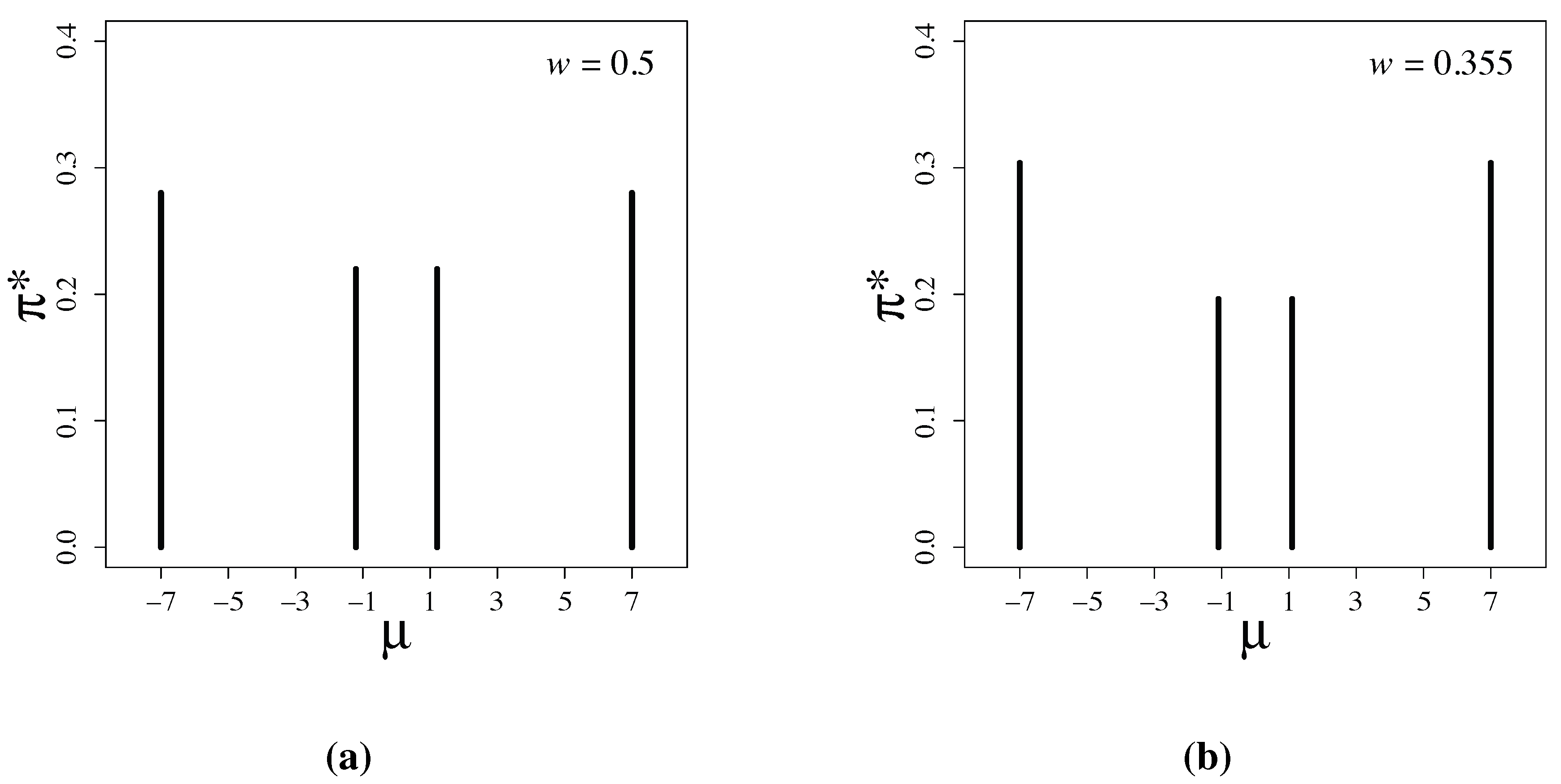
Figure 1. Latent information priors for (a) $w=0.5$ and for (b) $w=0.355$.

Figure 1. Latent information priors for (a) $w=0.5$ and for (b) $w=0.355$.

Figure 1 shows the numerically-obtained latent information priors. The priors have the form:

$$\begin{array}{c}\hfill {\pi }_w^{*}=\frac{u}{2}({\delta }_{-a}+{\delta }_a)+\frac{1-u}{2}({\delta }_{-b}+{\delta }_b)\end{array}$$

(18)

The parameter values are $a=1.21$, $b=7$ and $u=0.440$, when $w=0.5$, and $a=1.10$, $b=7$ and $u=0.393$, when $w=0.355$.

Lemma 2 below gives the risk of Bayesian testing based on the prior in Equation (18).

Lemma 2. 

Let:

$${\pi }_{a,b,u}=\frac{u}{2}({\delta }_{-a}+{\delta }_a)+\frac{1-u}{2}({\delta }_{-b}+{\delta }_b)$$

(19)

where $a,b>0$ and $0\le u\le 1$. Then, the risk in Equation (8) is given by:

$$\begin{array}{cc}& r_w(\mu ;{\pi }_{a,b,u})=-w\int \varphi \left(x\right)log\left\{1+\frac{1-w}{w}exp\left(-\frac{1}{2}{\mu }^2+\mu x\right)\right\}\mathrm{d}x\hfill \\ & -(1-w)\int \varphi \left(x\right)log\left\{1+\frac{w}{1-w}exp\left(-\frac{1}{2}{\mu }^2-\mu x\right)\right\}\mathrm{d}x\hfill \\ & +w\int \varphi \left(x\right)log\left\{1+\frac{1-w}{w}(1-u)exp\left(-\frac{1}{2}{b}^2\right)cosh\left(bx\right)+\frac{1-w}{w}uexp\left(-\frac{1}{2}{a}^2\right)cosh\left(ax\right)\right\}\mathrm{d}x\hfill \\ \text{(20)}\hfill & & +(1-w)\int \varphi (x-\mu )log\left\{1+\frac{w}{1-w}\frac{1}{(1-u)exp\left(-\frac{1}{2}{b}^2\right)cosh\left(bx\right)+uexp\left(-\frac{1}{2}{a}^2\right)cosh\left(ax\right)}\right\}\mathrm{d}x\hfill \end{array}$$

and the conditional mutual information in Equation (1) is given by:

$$\begin{array}{cc}& I_{m;\mu \mid x}(w,{\pi }_{a,b,u})=u[-w\int \varphi \left(x\right)log\left\{1+\frac{1-w}{w}exp\left(-\frac{1}{2}{a}^2-ax\right)\right\}\mathrm{d}x\hfill \\ & -(1-w)\int \varphi \left(x\right)log\left\{1+\frac{w}{1-w}exp\left(-\frac{1}{2}{a}^2-ax\right)\right\}\mathrm{d}x]\hfill \\ & +(1-u)[-w\int \varphi \left(x\right)log\left\{1+\frac{1-w}{w}exp\left(-\frac{1}{2}{b}^2-bx\right)\right\}\mathrm{d}x\hfill \\ & -(1-w)\int \varphi \left(x\right)log\left\{1+\frac{w}{1-w}exp\left(-\frac{1}{2}{b}^2-bx\right)\right\}\mathrm{d}x]\hfill \\ & +w\int \varphi \left(x\right)log\left\{1+\frac{1-w}{w}uexp\left(-\frac{1}{2}{a}^2\right)cosh\left(ax\right)+\frac{1-w}{w}(1-u)exp\left(-\frac{1}{2}{b}^2\right)cosh\left(bx\right)\right\}\mathrm{d}x\hfill \\ & +(1-w)u\int \varphi (x-a)log\left\{1+\frac{w}{1-w}\frac{1}{(1-u)exp\left(-\frac{b^2}{2}\right)cosh\left(bx\right)+uexp\left(-\frac{a^2}{2}\right)cosh\left(ax\right)}\right\}\mathrm{d}x\hfill \\ \text{(21)}\hfill & & +(1-w)(1-u)\int \varphi (x-b)log\left\{1+\frac{w}{1-w}\frac{1}{(1-u)exp\left(-\frac{b^2}{2}\right)cosh\left(bx\right)+uexp\left(-\frac{a^2}{2}\right)cosh\left(ax\right)}\right\}\mathrm{d}x\hfill \end{array}$$

The first and second terms in Equation (20) do not depend on π. The third term in Equation (20) does not depend on μ.

Figure 2 shows the risk functions of the latent information priors when $w=0.5$ and $w=0.355$, respectively. Note that ${max}_{\mu \in [-b,b]}{r}_w(\mu ,{\pi }^{*})$ is attained at $\mu =a$ and b in both examples. This is consistent with the proof of Theorem 1, and it is numerically verified that the prior maximizes the conditional mutual information. Furthermore, we observe that the supremum value, ${sup}_{\mu \in \mathbb{R}}{r}_w(\mu ,{\pi }^{*})$, of the risk without restriction $\mu \in [-b,b]$ is only slightly larger than the maximum value, ${max}_{\mu \in [-b,b]}{r}_w(\mu ,{\pi }^{*})$, with the restriction $\mu \in [-b,b]$. The risk functions rapidly converge as μ exceeds seven.

Figure 2. Risk functions of Bayesian testing based on latent information priors for (a) $w=0.5$ and for (b) $w=0.355$. When $w=0.5$, $a=1.21$ and $b=7$. When $w=0.355$, $a=1.10$ and $b=7$. The vertical dotted lines indicate the locations of a and b.

Figure 2. Risk functions of Bayesian testing based on latent information priors for (a) $w=0.5$ and for (b) $w=0.355$. When $w=0.5$, $a=1.21$ and $b=7$. When $w=0.355$, $a=1.10$ and $b=7$. The vertical dotted lines indicate the locations of a and b.

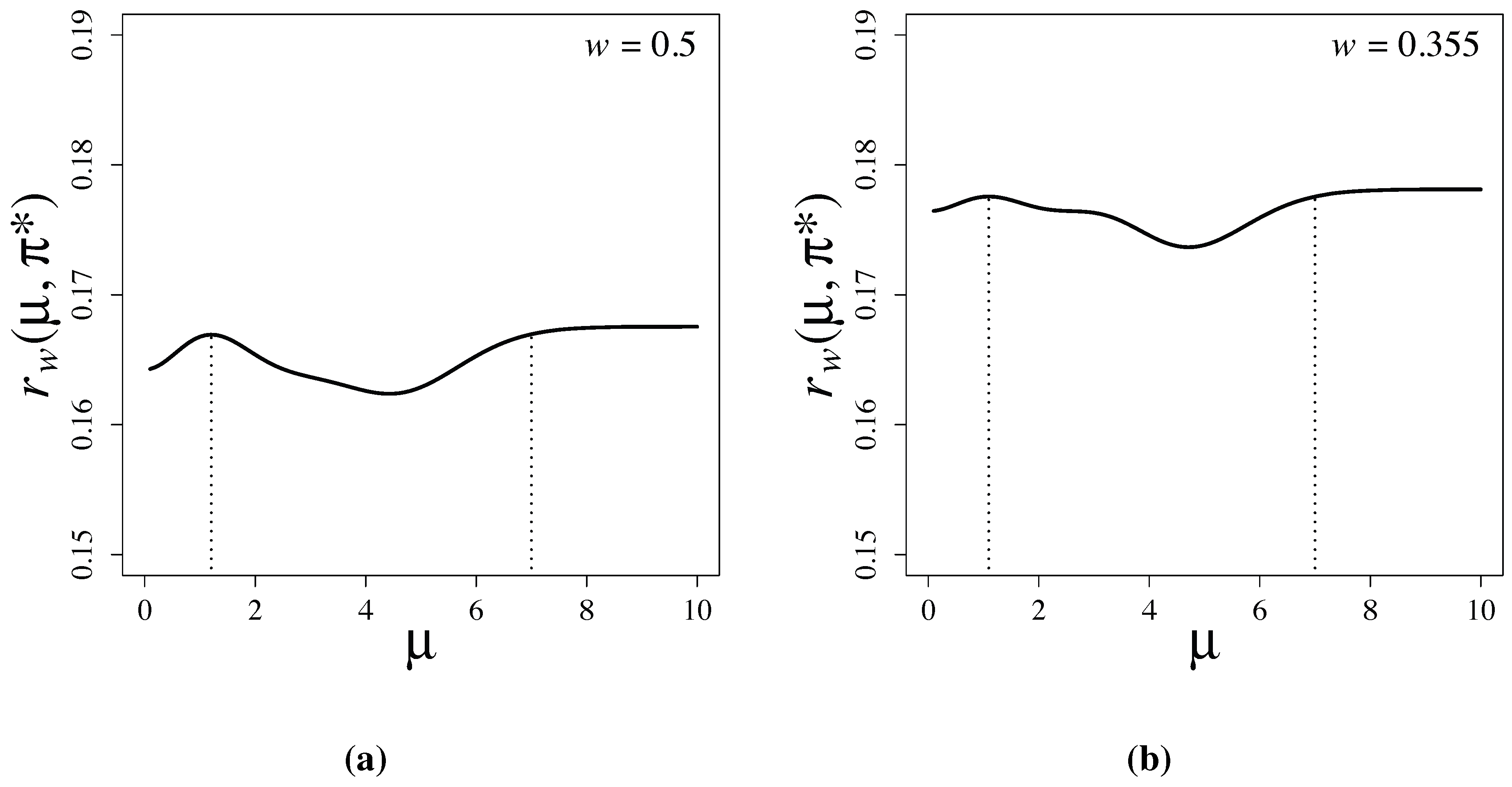
Since:

$$\begin{array}{cc}\hfill \underset{\mu \in K}{sup}& r(\mu ,{\pi }^{*})=\underset{{\pi }^{\prime }\in \mathcal{P}\left(K\right)}{sup}\underset{\pi \in \mathcal{P}\left(K\right)}{inf}R({\pi }^{\prime },\pi )=\underset{{\pi }^{\prime }\in \mathcal{P}\left(K\right)}{sup}\underset{\pi \in \mathcal{P}\left(\mathbb{R}\right)}{inf}R({\pi }^{\prime },\pi )\hfill \end{array}$$

$$\begin{array}{cc}\hfill \le & \underset{{\pi }^{\prime }\in \mathcal{P}\left(\mathbb{R}\right)}{sup}\underset{\pi \in \mathcal{P}\left(\mathbb{R}\right)}{inf}R({\pi }^{\prime },\pi )\le \underset{\pi \in \mathcal{P}\left(\mathbb{R}\right)}{inf}\underset{{\pi }^{\prime }\in \mathcal{P}\left(\mathbb{R}\right)}{sup}R({\pi }^{\prime },\pi )=\underset{\pi \in \mathcal{P}\left(\mathbb{R}\right)}{inf}\underset{\mu \in \mathbb{R}}{sup}r(\mu ,\pi )\le \underset{\mu \in \mathbb{R}}{sup}r(\mu ,{\pi }^{*})\hfill \end{array}$$

(22)

and ${sup}_{\mu \in \mathbb{R}}r(\mu ,{\pi }^{*})-{sup}_{\mu \in K}r(\mu ,{\pi }^{*})$ is small in our problem when $K=[-b,b]$$(b=7)$, the supremum value, ${sup}_{\mu \in \mathbb{R}}r(\mu ,{\pi }^{*})$, of the risk function of the latent information prior, ${\pi }^{*}$, under the parameter restriction, $\mu \in [-7,7]$, is only slightly larger than the minimax value, ${inf}_{\pi \in \mathcal{P}\left(\mathbb{R}\right)}{sup}_{\mu \in \mathbb{R}}r(\mu ,\pi )$ without the restriction. We see in the next section that the supremum, ${sup}_{\mu \in \mathbb{R}}r(\mu ,\pi )$, of the risk functions of commonly used priors are much larger than those of ${\pi }^{*}$.

The discreteness of latent information priors shown in Figure 1 is a remarkable feature. In Bayesian statistics, k-reference priors have been known to be discrete measures in many examples; see [11,12,13]. The k-reference prior is defined to be a prior maximizing the mutual information between $x^k$ and θ when we have a set, $x^k$, of k-independent observations, $x_1,\dots ,x_k$, from $p(x\mid \theta )$ in a parametric model, $\{p(x\mid \theta )\mid \theta \in \Theta \subset {\mathbb{R}}^d\}$. However, such discrete priors have not been widely used. Instead of k-reference priors, reference priors introduced by Bernardo [14] have been used for many problems. Reference priors are not discrete and are defined by considering the limit that the sample size k goes to infinity. One main reason why discrete priors are not popular is that discrete priors are totally unacceptable form the viewpoint of subjective Bayes in which priors are considered to represent prior belief on parameters.

Although they have not been widely used, discrete priors, such as latent information priors, are reasonable from the viewpoint of prediction and objective Bayes. Various statistical problems, including estimation and testing, can be formulated from the viewpoint of prediction, and priors can be constructed by considering the conditional mutual information. Thus, latent information priors depending on the choice of variables to be predicted could play important roles in many statistical applications. Conditional mutual information is essential in information theory and naturally appeared in several studies in statistics; see e.g., [15,16]. Priors based on conditional mutual information and those based on unconditional mutual information are often quite different; see [4].

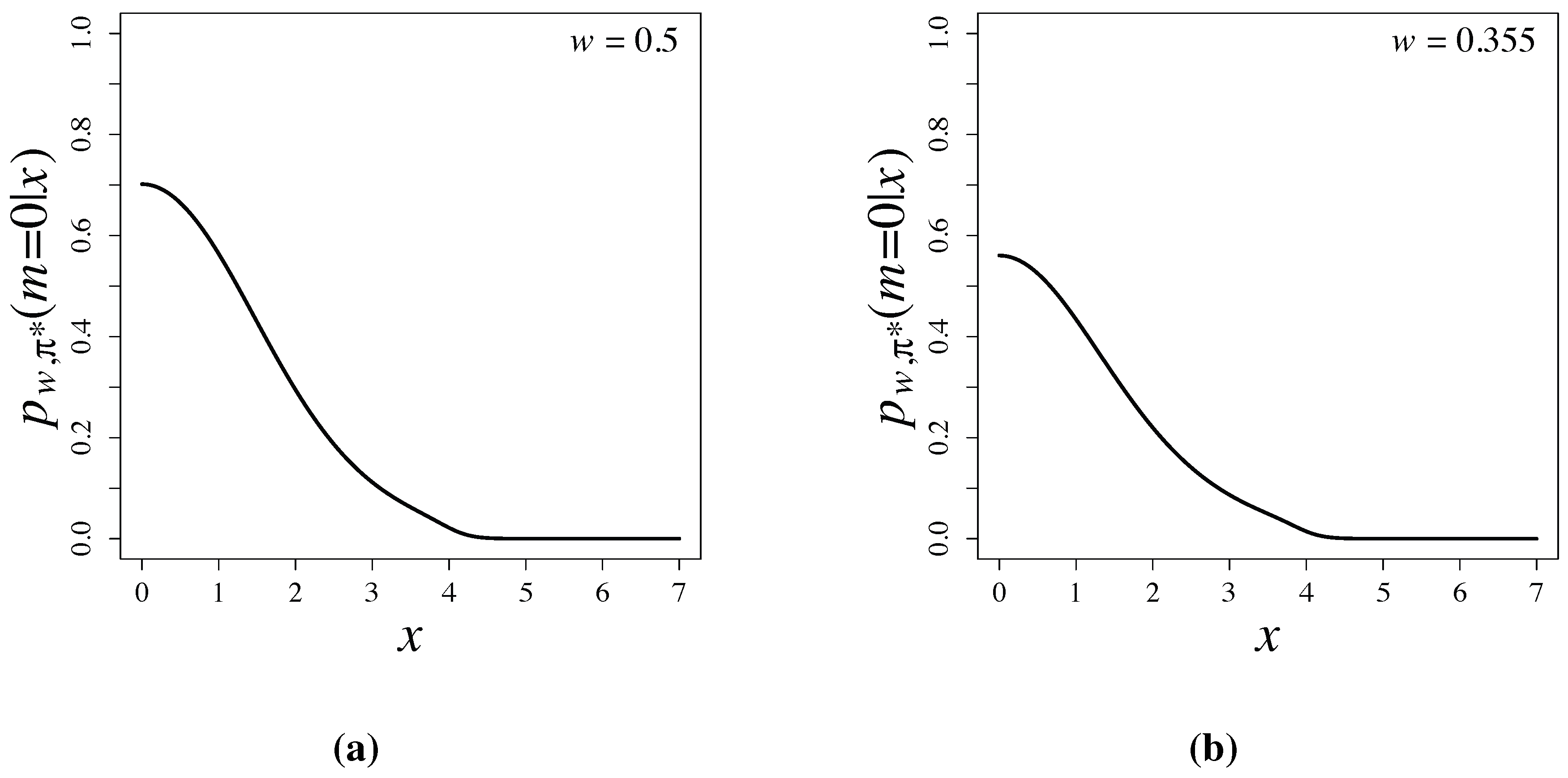
Bayesian testing based on latent information priors is free from the Jeffreys-Lindley paradox [3], since the priors are constructed by using conditional mutual information and depend properly on sample sizes. Posterior probabilities, $p_{w,{\pi }^{*}}(m=0\mid x)$, are shown in Figure 3 and are compared with p-values of the two-sided test in Table 1. When $x=2,3$ and 4, posterior probabilities are much smaller than p-values of the two-sided test. Large differences of posterior probabilities and p-values have been widely observed and discussed in [1,17,18].

Figure 3. Posterior probabilities $p_{w,{\pi }^{*}}(m=0\mid x)$ based on latent information priors for (a) $w=0.5$ and for (b) $w=0.355$.

Figure 3. Posterior probabilities $p_{w,{\pi }^{*}}(m=0\mid x)$ based on latent information priors for (a) $w=0.5$ and for (b) $w=0.355$.

Table 1. Comparison of posterior probabilities and p-values.

x	0	1	2	3	4
$p_{w=0.5}(m=0\mid x)$	0.702	0.564	0.295	0.112	0.0217
$p_{w=0.355}(m=0\mid x)$	0.560	0.434	0.220	0.0867	0.0145
p-value (two-sided test)	1	0.317	0.0455	0.00267	$6.33\times {10}^{-5}$

Table 1. Comparison of posterior probabilities and p-values.

x	0	1	2	3	4
$p_{w=0.5}(m=0\mid x)$	0.702	0.564	0.295	0.112	0.0217
$p_{w=0.355}(m=0\mid x)$	0.560	0.434	0.220	0.0867	0.0145
p-value (two-sided test)	1	0.317	0.0455	0.00267	$6.33\times {10}^{-5}$

4. Other Common Priors

Discrete priors, including latent information priors discussed in the previous section, have not been widely used in Bayesian statistics. Common priors for the testing are the normal prior and the Cauchy prior. It seems to have been believed by many statisticians that the Cauchy prior is slightly better than the normal prior; see, e.g., [1,2]. In this section, we evaluate the conditional mutual information for the priors and compare the performance of them to that of the latent information prior.

4.1. The Normal Prior

The normal prior, $\varphi (\mu ;0,{\tau }^2)$, is denoted by ${\mathrm{N}}_{\tau }$. From Lemma 1, we have:

$$\begin{array}{cc}\hfill r_w(\mu ,{\mathrm{N}}_{\tau })=& -w\int \varphi (x;0,1)log\left\{1+\frac{1-w}{w}exp\left(-\frac{1}{2}{\mu }^2+\mu x\right)\right\}\mathrm{d}x\hfill \\ & -(1-w)\int \varphi (x;0,1)log\left\{1+\frac{w}{1-w}exp\left(-\frac{1}{2}{\mu }^2-\mu x\right)\right\}\mathrm{d}x\hfill \\ & +w\int \varphi (x;0,1)log\left\{1+\frac{1-w}{w}\frac{\varphi (x;0,{\tau }^2+1)}{\varphi (x;0,1)}\right\}\mathrm{d}x\hfill \\ \text{(23)}\hfill & & +(1-w)\int \varphi (x;\mu ,1)log\left\{1+\frac{w}{1-w}\frac{\varphi (x;0,1)}{\varphi (x;0,{\tau }^2+1)}\right\}\mathrm{d}x\hfill \end{array}$$

Thus, the conditional mutual information is given by:

$$\begin{array}{cc}\hfill I_{m;\mu \mid x}& (w,{\mathrm{N}}_{\tau })=\int r_w(\mu ,{\mathrm{N}}_{\tau })\varphi (\mu ;0,{\tau }^2)\mathrm{d}\mu \hfill \\ \hfill =& -w\int \varphi (x;0,1)\varphi (\mu ;0,{\tau }^2)log\left\{1+\frac{1-w}{w}exp\left(-\frac{1}{2}{\mu }^2+\mu x\right)\right\}\mathrm{d}\mu \mathrm{d}x\hfill \\ & -(1-w)\int \varphi (x;0,1)\varphi (\mu ;0,{\tau }^2)log\left\{1+\frac{w}{1-w}exp\left(-\frac{1}{2}{\mu }^2-\mu x\right)\right\}\mathrm{d}\mu \mathrm{d}x\hfill \\ & +w\int \varphi (x;0,1)log\left\{1+\frac{1-w}{w}\frac{\varphi (x;0,{\tau }^2+1)}{\varphi (x;0,1)}\right\}\mathrm{d}x\hfill \\ \text{(24)}\hfill & & +(1-w)\int \varphi (x;0,{\tau }^2+1)log\left\{1+\frac{w}{1-w}\frac{\varphi (x;0,1)}{\varphi (x;0,{\tau }^2+1)}\right\}\mathrm{d}x\hfill \end{array}$$

The conditional mutual information is evaluated by numerical integration. When $w=0.5$ and $w=0.355$, the maximum values:

$$\underset{\tau }{max}{I}_{m;\mu \mid x}(w=0.5,{\mathrm{N}}_{\tau })=0.156\text{and}\underset{\tau }{max}{I}_{m;\mu \mid x}(w=0.355,{\mathrm{N}}_{\tau })=0.166$$

(25)

of Equation (24) are attained at $\tau =4.92$ and $\tau =5.36$, respectively. The variation of the risk functions, $r_{w=0.5}(\mu ,{\mathrm{N}}_{\tau =4.92})$ and $r_{w=0.355}(\mu ,{\mathrm{N}}_{\tau =5.36})$, shown in Figure 4 are much larger than those of the risk functions of the latent information priors shown in Figure 2. Thus, the performance of the Bayesian testing based on the normal prior is worse than that based on the latent information prior if we adopt the Kullback-Leibler loss.

Figure 4. Risk functions of Bayesian testing based on normal priors for (a) $w=0.5$ and $\tau =4.92$; and for (b) $w=0.355$ and $\tau =5.36$. The functions have symmetry $r_w(-\mu ,{\mathrm{N}}_{\tau })=r_w(\mu ,{\mathrm{N}}_{\tau })$ about the origin.

Figure 4. Risk functions of Bayesian testing based on normal priors for (a) $w=0.5$ and $\tau =4.92$; and for (b) $w=0.355$ and $\tau =5.36$. The functions have symmetry $r_w(-\mu ,{\mathrm{N}}_{\tau })=r_w(\mu ,{\mathrm{N}}_{\tau })$ about the origin.

4.2. The Cauchy Prior

The Cauchy prior, $1/\left\{\gamma \pi ({\mu }^2/{\gamma }^2-1)\right\}$, is denoted by ${\mathrm{C}}_{\gamma }$. Since the characteristic functions of $\mathrm{N}(0,{\sigma }^2)$ and $C_{\gamma }$ are $exp\left(-\frac{1}{2}{\sigma }^2{t}^2\right)$ and $exp(-\gamma |t\left|\right)$, respectively, the characteristic function of the marginal density:

$$\begin{array}{c}\hfill p_{\mathrm{C}}(x\mid \gamma )=\int \frac{1}{\sqrt{2\pi {\sigma }^2}}exp\left\{-\frac{1}{2{\sigma }^2}{(x-\mu )}^2\right\}\frac{1}{\pi ({\mu }^2/{\gamma }^2-1)}\frac{1}{\gamma }\mathrm{d}\mu \end{array}$$

(26)

with respect to the Cauchy prior, ${\mathrm{C}}_{\gamma }$, is given by:

$$\begin{array}{c}\hfill exp\left(-\gamma \left|t\right|-\frac{1}{2}{t}^2\right)\end{array}$$

(27)

The expression:

$$\begin{array}{cc}\hfill p_{\mathrm{C}}(x\mid \gamma )=& \frac{1}{2\pi }{\int }_{-\infty }^{\infty }{\mathrm{e}}^{-\mathrm{i}xt}exp\left(-\gamma \left|t\right|-\frac{1}{2}{t}^2\right)\mathrm{d}t\hfill \\ \text{(28)}\hfill & \hfill =& \frac{1}{\sqrt{2\pi }\sigma }\mathrm{Re}\left[exp\left\{\frac{{(\mathrm{i}x-\gamma )}^2}{2}\right\}\text{erfc}\left(-\mathrm{i}\frac{x+\mathrm{i}\gamma }{\sqrt{2}}\right)\right]\hfill \end{array}$$

where $\mathrm{erfc}$ is the complementary error function defined by:

$$\begin{array}{cc}\hfill \text{erfc}\left(z\right)=& \frac{2}{\sqrt{\pi }}{\int }_z^{\infty }{\mathrm{e}}^{-t^2}\mathrm{d}t\hfill \end{array}$$

(29)

obtained by the inverse transform of Equation (27) is useful for numerical computation; see [19] (p. 183) and [20]. From Lemma 1, we have:

$$\begin{array}{cc}\hfill r_w(\mu ;C_{\gamma })=& -w\int \varphi (x;0,1)log\left\{1+\frac{1-w}{w}exp\left(-\frac{1}{2}{\mu }^2+\mu x\right)\right\}\mathrm{d}x\hfill \\ & -(1-w)\int \varphi (x;0,1)log\left\{1+\frac{w}{1-w}exp\left(-\frac{1}{2}{\mu }^2-\mu x\right)\right\}\mathrm{d}x\hfill \\ & +w\int \varphi (x;0,1)log\left\{1+\frac{1-w}{w}\frac{p_{\mathrm{C}}(x\mid \gamma )}{\varphi (x;0,1)}\right\}\mathrm{d}\epsilon \hfill \\ \text{(30)}\hfill & & +(1-w)\int \varphi (x;0,1)log\left\{1+\frac{w}{1-w}\frac{\varphi (x+\mu ;0,1)}{p_{\mathrm{C}}(x+\mu \mid \gamma )}\right\}\mathrm{d}x\hfill \end{array}$$

We numerically evaluate the conditional mutual information:

$$\begin{array}{cc}\hfill I_{m;\mu \mid x}(w,{\mathrm{C}}_{\gamma })=& \int r_w(\mu ;C_{\gamma })\frac{1}{\pi ({\mu }^2/{\gamma }^2-1)}\frac{1}{\gamma }\mathrm{d}\mu \hfill \end{array}$$

(31)

by the Monte-Carlo method. When $w=0.5$ and $w=0.355$, the maximum values:

$$\underset{\gamma }{max}{I}_{m;\mu \mid x}(w=0.5,{\mathrm{C}}_{\gamma })=0.161\text{and}\underset{\gamma }{max}{I}_{m;\mu \mid x}(w=0.355,{\mathrm{C}}_{\gamma })=0.170$$

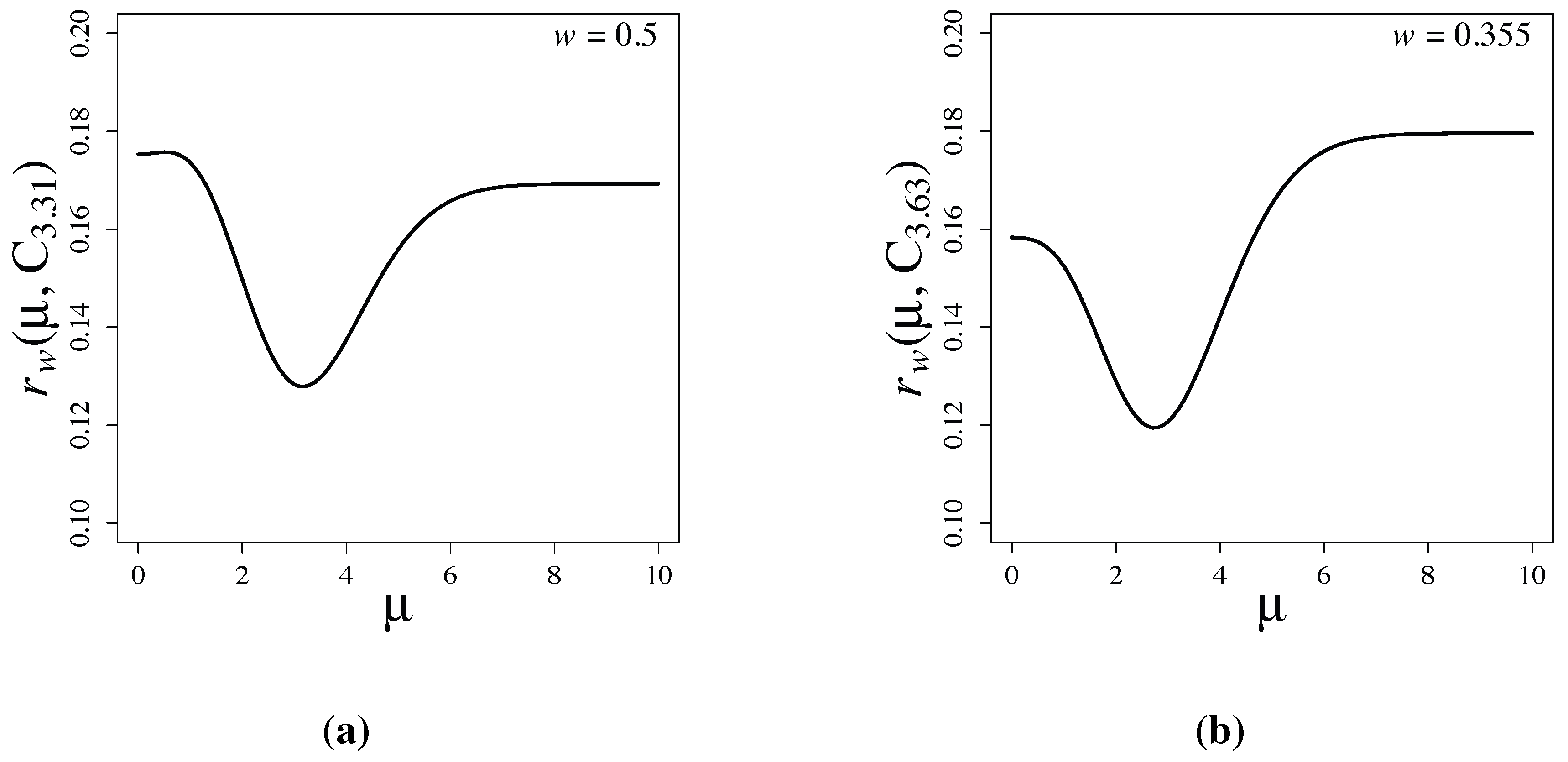
of Equation (31) are attained at $\gamma =3.31$ and $\gamma =3.63$, respectively. The risk functions $r_{w=0.5}(\mu ,{\mathrm{C}}_{\gamma =3.31})$ and $r_{w=0.355}(\mu ,{\mathrm{C}}_{\gamma =3.63})$ are shown in Figure 5. The variation of the risk function $r_{w=0.5}(\mu ,{\mathrm{C}}_{\gamma =3.31})$ is milder than that of the risk function $r_{w=0.5}(\mu ,{\mathrm{N}}_{\tau =4.92})$ based on the normal prior, and the inequality ${sup}_{\mu }{r}_{w=0.5}(\mu ,{\mathrm{C}}_{\gamma =3.31})<{sup}_{\mu }{r}_{w=0.5}(\mu ,{\mathrm{N}}_{\tau =4.92})$ holds. Thus, the Cauchy prior is preferable to the normal prior from the viewpoint of the Kullback-Leibler loss. However, the variation of the risk function shown in Figure 2 based on the latent information prior is much smaller than that of $r_{w=0.5}(\mu ,{\mathrm{C}}_{\gamma =3.31})$. Similar relations also hold when $w=0.355$.

Figure 5. Risk functions of Bayesian testing based on Cauchy priors for (a) $w=0.5$ and $\gamma =3.31$; and for (b) $w=0.355$ and $\gamma =3.63$. The functions have symmetry $r_w(-\mu ,{\mathrm{C}}_{\gamma })=r_w(\mu ,{\mathrm{C}}_{\gamma })$ about the origin.

Figure 5. Risk functions of Bayesian testing based on Cauchy priors for (a) $w=0.5$ and $\gamma =3.31$; and for (b) $w=0.355$ and $\gamma =3.63$. The functions have symmetry $r_w(-\mu ,{\mathrm{C}}_{\gamma })=r_w(\mu ,{\mathrm{C}}_{\gamma })$ about the origin.

5. Conclusions

We discussed the use of latent information priors for Bayesian testing of a point null hypothesis. The testing problem was formulated as a prediction problem, and latent information priors were numerically obtained. The variations of the risk functions of latent information priors are much smaller than those of normal and Cauchy priors. Although the testing problem treated in the present paper is simple, the results may indicate that latent information priors could be useful for various problems, since many statistical problems can be formulated from the viewpoint of prediction.

When the parameter space is multidimensional, it becomes difficult to numerically obtain latent information priors, and some approximations need to be used. One possible approach is to use asymptotic methods, and another possible approach is to choose an approximating prior from a tractable subset of the set of all probability measures on the parameter space. These approaches require further investigation.

References

- Berger, J.O.; Sellke, T. Testing a point null hypothesis: The irreconcilability of p values and evidence. J. Am. Stat. Assoc. 1987, 82, 112–122. [Google Scholar] [CrossRef]
- Jeffreys, H. Theory of Probability, 3rd ed.; Oxford University Press: Oxford, UK, 1961. [Google Scholar]
- Lindley, D.V. A statistical paradox. Biometrika 1957, 44, 187–192. [Google Scholar] [CrossRef]
- Komaki, F. Bayesian predictive densities based on latent information priors. J. Stat. Plan. Inference 2011, 141, 3705–3715. [Google Scholar] [CrossRef]
- Aitchison, J. Goodness of prediction fit. Biometrika 1975, 62, 547–554. [Google Scholar] [CrossRef]
- Csiszár, I. I-divergence geometry of probability distributions and minimization problems. Ann. Probab. 1975, 3, 146–158. [Google Scholar] [CrossRef]
- Haussler, D. A general minimax result for relative entropy. IEEE Trans. Inf. Theory 1997, 43, 1276–1280. [Google Scholar] [CrossRef]
- Grünwald, P.D.; Dawid, A.P. Game theory, maximum entropy, minimum discrepancy and robust Bayesian decision theory. Ann. Stat. 2004, 32, 1367–1433. [Google Scholar]
- Arimoto, S. An algorithm for computing the capacity of arbitrary discrete memoryless channels. IEEE Trans. Inf. Theory 1972, 18, 14–20. [Google Scholar] [CrossRef]
- Blahut, R. Computation of channel capacity and rate-distortion functions. IEEE Trans. Inf. Theory 1972, 18, 460–473. [Google Scholar] [CrossRef]
- Hartigan, J.A. Bayes Theory; Springer: New York, NY, USA, 1983. [Google Scholar]
- Berger, J.; Bernardo, J.M.; Mendoza, M. On Priors that Maximize Expected Information. In Recent Developments in Statistics and Their Applications; Klein, J.P., Lee, J.C., Eds.; Freedom Press: Seoul, Korea, 1989; pp. 1–20. [Google Scholar]
- Zhang, Z. Discrete Noninformative Priors. Ph.D. Dissertation, Department of Statistics, Yale University, New Haven, CT, USA, 1994. [Google Scholar]
- Bernardo, J.M. Reference posterior distributions for Bayesian inference. J. R. Stat. Soc. B 1979, 41, 113–147. [Google Scholar]
- Clarke, B.; Yuan, A. Partial information reference priors: Derivation and interpretations. J. Stat. Plan. Inference 2004, 123, 313–345. [Google Scholar] [CrossRef]
- Ebrahimi, N.; Soofi, E.S.; Soyer, R. On the sample information about parameter and prediction. Stat. Sci. 2010, 25, 348–367. [Google Scholar] [CrossRef]
- Edwards, W.; Lindman, H.; Savage, L.J. Bayesian statistical inference for psychological research. Psychol. Rev. 1963, 70, 193–242. [Google Scholar] [CrossRef]
- Dickey, J.M. Is the tail area useful as an approximate Bayes factor? J. Am. Stat. Assoc. 1977, 72, 138–142. [Google Scholar] [CrossRef]
- Temme, N.M. Error Functions, Dawson’s and Fresnel Integrals. In NIST Handbook of Mathematical Functions; Olver, F.W.J., Lozier, D.W., Boisvert, R.F., Clark, C.W., Eds.; Cambridge University Press: Cambridge, UK, 2010; pp. 159–171. [Google Scholar]
- Poppe, G.P.M.; Wijers, C.M.J. Algorithm 680: Evaluation of the complex error function. ACM Trans. Math. Softw. (TOMS) 1990, 16. [Google Scholar] [CrossRef]
Appendix. Proofs of Lemmas
Proof of Lemma 1. From Equation (8), we have:
because m and μ are independent. Since:
and:
we have:
Proof of Lemma 2. Since:
From Lemma 1, we have:
The conditional mutual information is:
From Equations (38) and (39), we obtain the desired result. ☐
© 2013 by the author; licensee MDPI, Basel, Switzerland. This article is an open access article distributed under the terms and conditions of the Creative Commons Attribution license (http://creativecommons.org/licenses/by/3.0/).
Share and Cite
MDPI and ACS Style
Komaki, F. Bayesian Testing of a Point Null Hypothesis Based on the Latent Information Prior. Entropy 2013, 15, 4416-4431. https://doi.org/10.3390/e15104416
AMA Style
Komaki F. Bayesian Testing of a Point Null Hypothesis Based on the Latent Information Prior. Entropy. 2013; 15(10):4416-4431. https://doi.org/10.3390/e15104416
Chicago/Turabian StyleKomaki, Fumiyasu. 2013. "Bayesian Testing of a Point Null Hypothesis Based on the Latent Information Prior" Entropy 15, no. 10: 4416-4431. https://doi.org/10.3390/e15104416