All Shook Up: Fluctuations, Maxwell’s Demon and the Thermodynamics of Computation

Department of History and Philosophy of Science, Center for Philosophy of Science, University of Pittsburgh, Pittsburgh, PA 15260, USA
Entropy 2013, 15(10), 4432-4483; https://doi.org/10.3390/e15104432
Submission received: 3 July 2013
/
Revised: 17 September 2013
/
Accepted: 22 September 2013
/
Published: 17 October 2013
(This article belongs to the Special Issue Maxwell’s Demon 2013)
Abstract
:The most successful exorcism of Maxwell’s demon is Smoluchowski’s 1912 observation that thermal fluctuations would likely disrupt the operation of any molecular-scale demonic machine. A later tradition sought to exorcise Maxwell’s demon by assessing the entropic cost of the demon’s processing of information. This later tradition fails since these same thermal fluctuations invalidate the molecular-scale manipulations upon which the thermodynamics of computation is based. A new argument concerning conservation of phase space volume shows that all Maxwell’s demons must fail.
1. Introduction
Maxwell’s demon threatens to overturn the second law of thermodynamics by manipulating individual molecules in a way that assures a reduction in thermodynamic entropy. The view now standard is that the demon must fail because of a compensating dissipation associated with the processing of information, necessary for the proper functioning of the demon. This standard view calls upon a new science, the thermodynamics of computation, and locates the compensating dissipation in the k ln 2 of thermodynamic entropy that Landauer’s principle asserts must be passed to the environment each time a bit of information is erased.
Here is how this consensus appears in a recent letter to Nature in which experimental validation of Landauer’s principle is announced [1]:
The paradox of the apparent violation of the second law can be resolved by noting that during a full thermodynamic cycle, the memory of the demon, which is used to record the coordinates of each molecule, has to be reset to its initial state. Indeed, according to Landauer’s principle, any logically irreversible transformation of classical information is necessarily accompanied by the dissipation of at least kTln(2) of heat per lost bit (about 3 × 10⁻²¹ J at room temperature (300 K)), where k is the Boltzmann constant and T is the temperature.… This entropy cost required to reset the demon’s memory to a blank state is always larger than the initial entropy reduction, thus safeguarding the second law. Landauer’s principle hence seems to be a central result that not only exorcizes Maxwell’s demon, but also represents the fundamental physical limit of irreversible computation.
This consensus appears to provide a quite satisfying resolution of an enduring challenge to a fundamental physical principle. The challenge is defeated by discovery of a profound connection between information and thermodynamics, as codified in the new science of the thermodynamics of computation. There is a comfortable sense in the literature of maturity and stability.
There is another, dimmer view of this resolution. (For a direct response to Bérut et al.’s [1] claim of experimental validation, see Section 3.7 below.) In this dissenting view, the exorcism is not based on the discovery of any new physical principle, but on circular reasoning. It starts with the assumption that there are no exceptions to the second law and uses that assumption to generate Landauer’s principle. After some detours, that same assumption is returned, now disguised as the discovery that Maxwell’s demon cannot be the exception. The detours include one or two suggestive thought experiments in which the exact quantities of entropy destroyed by the demon reappear magically in the erasure of information. From these few cases, we are to extrapolate extravagantly and conclude every conceivable demonic device must succumb through repetition of this magical agreement, even if the demonic device in no way resembles a computer with a discrete memory that requires erasure.
Worse, the new science of the thermodynamics of computation is no science at all. It depends on a principle that is not well-founded, but merely a supposition that has become established through the comfort of frequent repetition. Its proofs are not proofs, but flawed plausibility arguments or elaborate demonstrations whose convolutions hide their dependence on the same few misapplications of thermodynamics. It is all a mirage that appears real from a distance but dissolves when we approach it more closely.
The natural appeal of a connection between information and thermodynamics has, in the end, had a quite harmful effect on our understanding of the prospects of Maxwell’s demon. For it has eclipsed one of the most successful exorcisms. The modern tradition in Maxwell’s demon began with the acceptance in the early 20th century of the molecular basis of thermal phenomena. This basis entailed the existence of thermal fluctuations, such as Brownian motion. They were identified as molecular-scale violations of the second law of thermodynamics. If these molecular-scale violations could be accumulated sufficiently, we would have a macroscopic violation. Seeking a device that would accumulate them became the guiding design principle upon which a new generation of proposals for Maxwell’s demon was based. In 1912, Smoluchowski diagnosed why these proposals would fail. He showed that, in a broad selection of proposals, further thermal fluctuations would fatally disrupt the intended functioning of the device proposed. For each process that could accumulate violations of the second law, there would be another, also derived from fluctuations, that would undo it.
Smoluchowski’s analysis gives the best physical understanding of why a Maxwell’s demon must fail, if it must. The molecular-scale world is quite unlike that of our macroscopic experience. Each molecular-scale component has its own thermal energy that leads it to bounce around in all its degrees of freedom. Those molecular motions overturn our macroscopic intuitions about how delicate, molecular-scale machinery operates and defeat apparently natural designs for demons.
This paper has two parts. The first describes three attempts to exorcise Maxwell’s demon. Smoluchowski’s fluctuation based exorcism is described in Section 2. Section 3 describes the modern version of the information-theoretic exorcisms of Maxwell’s demon. It depends upon Landauer’s principle and the thermodynamics of computation. A minority view, critical of this exorcism, appears in several versions in the literature. This section will summarize the version that I have developed in earlier papers, initially in collaboration with John Earman. It is critical of the exorcism at the general level, arguing that it is both circular and too heavily dependent on a few examples of dubious generality. It is also judges the thermodynamics of computation and its central principle, Landauer’s principle, to be defective in its foundations.
Section 4 will develop what I believe is a new, simple and quite robust exorcism of Maxwell’s demon. Maxwell’s demon is presumed always or very likely to succeed in reversing the second law of thermodynamics, when placed in a generic thermal environment. The presumption that it succeeds always or even just mostly may seem innocuous initially. However it proves to be far too strong a requirement, for it conflicts with the conservation of phase volume in Hamiltonian dynamics.
Part II of this paper revives Smoluchowski’s insight of the controlling influence of fluctuations at molecular scales. It presents the fullest development so far of a no-go result that dissolves the thermodynamics of computation. That field is based on the assumption that all molecular-scale computational operations, excepting erasure and other logically irreversible processes, can be implemented as thermodynamically reversible processes. The results shows that, on the contrary, each attempt to implement a thermodynamically reversible process on the molecular scale will be disrupted by thermal fluctuations or, to use the circuit-theoretic term, thermal noise. Completion of a single computational step can only be achieved, it is shown, with the introduction of thermodynamic entropy creating disequilibria, where the entropy created exceeds the k ln 2 tracked by Landauer’s principle. The standard computational architecture requires a sequence of steps, each of which must be completed before the next is initiated. This entropy creation is required in each step. As a result, the minimum creation of thermodynamic entropy is not determined by the logical specification of the computation. It depends merely on the number of discrete steps that must be completed.
In the early sections of Part II, the premises of the result are laid our more fully, including the assumption that the thermodynamically reversible processes intended for use in molecular-scale computation must be self-contained. Later sections include several new illustrations of the result.
Part 1. Three Exorcisms of Maxwell’s Demon
2. Fluctuation Based Exorcisms of Maxwell’s Demon: A Historical Review
2.1. Thermal Fluctuations Challenge the Second Law of Thermodynamics
Since its conception by Maxwell in the 1860s, his demon has enjoyed a rich history. Here I recall one historical episode. It provides one of the best explanations of why Maxwell’s demon will likely fail. This exorcism has faded in the present literature and needs to be revived.
Maxwell had not originally conceived his demon as something that could be realized practically (for a recent, highly informative account of Maxwell’s conception, see Myrvold [2]. That changed at the start of the 20th century with the serious investigation of thermal fluctuations. They are the ever-varying, probabilistically-governed deviations of the thermal properties of small systems from their mean values, as predicted by the molecular-kinetic theory of heat. In his celebrated analysis of Brownian motion as a thermal fluctuation process, Einstein [3] remarked (p. 49) with some understatement that, if the predicted motions of small corpuscles really were observed, then “classical thermodynamics can no longer be taken as exactly valid for microscopically distinguishable spaces.” In a lecture of September 24, 1904, Poincaré [4] had spoken (p. 610) more provocatively of the thermal motions of pollen grains, visible under the microscope:
[…] we see under our eyes now motion transformed into heat by friction, now heat changed inversely into motion, and that without loss since the movement lasts forever. This is the contrary of the principle of Carnot.If this be so, to see the world return backward, we no longer have need of the infinitely keen eye of Maxwell's demon; our microscope suffices us.
If we suppose the molecular kinetic theory correct, fluctuation phenomena would be, on Poincaré’s authority, microscopic violations of the second law of thermodynamics (“principle of Carnot”). They were real and microscopically visible. All that was needed, it seemed, was for some device that could accumulate these many small violations of the law into a single big violation.
Here I take the second law of thermodynamics to be the principle introduced by Thomson [5] (pp. 179, 181) in equivalent forms: “It is impossible, by means of inanimate material agency, to derive mechanical effect from any portion of matter by cooling it below the temperature of the coldest of the surrounding objects.” (Thomson form) “It is impossible for a self-acting machine, unaided by any external agency, to convey heat from one body to another at a higher temperature.” (Clausius form)
2.2. Fluctuation Demons…
Seeking out such physical realizations of Maxwell’s demon and an analysis of whether they can really work became a serious topic in physics. For a fuller discussion of the proposals and analyses, see Earman and Norton [6]. Here I will describe several of the proposals from the time and sketch the consensus that developed for why they must fail. In brief, it turned out that for any process in which fluctuations were used to attempt a violation of the second law, there would be a second process, also driven by fluctuations that would undo the violation.
One of the demonic devices proposed in Svedberg [7] sought to exploit the endless Brownian motion of colloidal particles. They can carry a charge, Svedberg noted, and since they jostle back and forth, their motion is accelerating. Therefore, they must be radiating electromagnetically, as do charges in a radio transmitter antenna. That is, the thermal energy of the colloids at ambient temperature is radiated out into space. Might we capture that energy and use it to heat something above ambient temperature?
To realize such a device, Svedberg proposed that the colloidal solution be contained within a glass vessel that would in turn be surrounded by a lead casing or shield; and the lead casing would be tuned in size to maximize the absorption of the electromagnetic waves emitted by the radiating colloidal particles. The outcome would be that the lead casing grows warmer as it absorbs the radiation. This warming comes at the expense of energy drawn from the motion of the colloidal particles, which must as a result be slowed. Their Brownian motion would be restored by the thermal energy of the solvent in which they are suspended. So the solvent cools. The outcome would be a process whose overall effect is the cooling of one body while its environment is heated, in direct violation of the second law of thermodynamics.
Svedberg’s device is sketched in Figure 1. The sketch omits many of the details of Svedberg’s design. It included an additional lead casing, several water casings and also two vacuum layers, all designed to assure that the demon operates as intended. The vacuum layers, for example, preclude heat being conducted back from the heated lead layer to the cooling colloid. The level of detail of Svedberg’s description reflects that this was a serious proposal.
Figure 1.
Svedberg’s colloid demon.

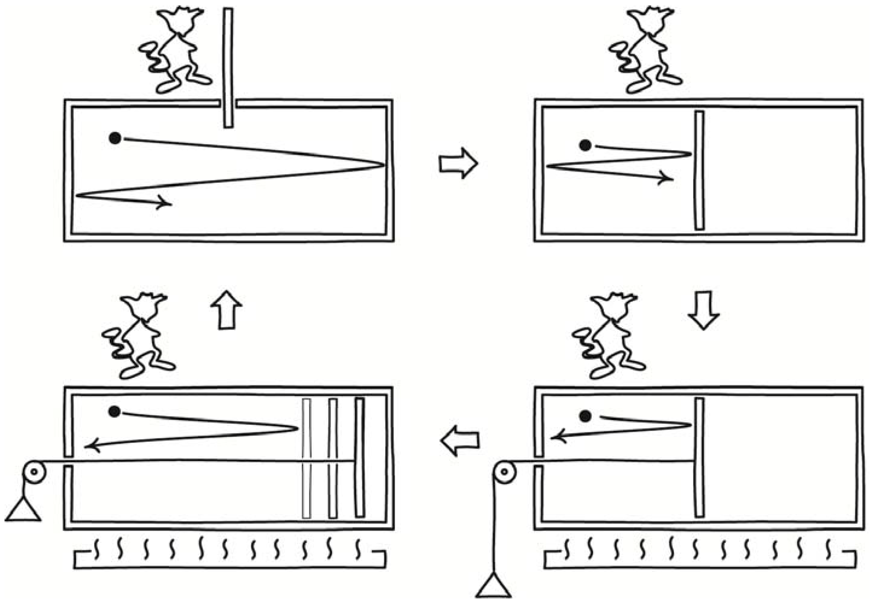
Svedberg left open the question of whether such devices really can overturn the second law of thermodynamics. Marian Smoluchowski took up that challenge of answering that question in a paper of 1912. There he described several more demonic devices. The most familiar of these later came to be known as the “Smoluchowski trapdoor.” In his original version [8] (Section III), a hole in a partition dividing a gas chamber was fitted with a ring of hairs or a one-way valve that would permit the gas to pass one way only. See Figure 2. Gas molecules proceeding from left to right collide with the valve’s flapper, lift it and pass. Gas molecules proceeding from right to left collide with the flapper and close it, obstructing their passage.
Figure 2.
Smoluchowski’s valve demon.

While it may not be immediately apparent, this device is still exploiting fluctuations. For it is the fluctuations in pressure on the flapper of a swing check valve due to molecular collisions that lead the valve to open. The effect should be that gas molecules pass preferentially in one direction, spontaneously producing a pressure differential that could be used to do work. The source of the work energy is the thermal energy of the gas, which is converted fully into work. The process would violate the second law of thermodynamics.
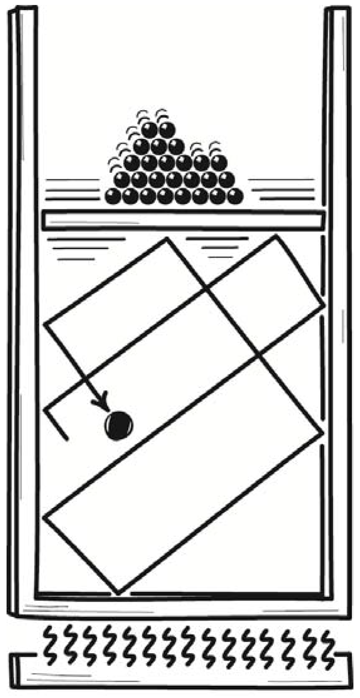
A small variant of the same idea was a toothed wheel that would rotate back and forth through thermal fluctuations. It is the analog in angular motion of the linear Brownian motion of colloids. A spring-loaded pawl, however, would engage the teeth and only permit the wheel to turn in one direction, as shown in Figure 3. As it turned, it would slowly wind up a torsion spring. The energy of the spring would be derived from the kinetic energy of the wheel, which would in turn be replenished by the thermal energy of the surroundings. That is a full conversion of ambient heat to work, again in violation of the second law. This example was later included in Feynman’s celebrated textbook [9] in Chapter 46.
Figure 3.
Smoluchowski’s toothed wheel and pawl demon.

Finally, Smoluchowski described an electrical demon. He considered an electrically charged air condenser, that is, one whose dielectric is just an air space, as shown in Figure 4. It is connected through a resistor to ground. The capacitance of the condenser varies continuously because of thermally induced fluctuations in the density of the air forming the condenser’s dielectric. Since its charge is fixed, the voltage of the condenser would fluctuate; and this would lead to small currents in the resistor. The energy of these currents would be converted to heat in the resistor, which would be warmed by the process to a temperature above that of the surroundings. The energy warming the resistor would be derived ultimately from the thermal energy of air, as it maintained the fluctuations in the condenser. Once again the second law is violated.
Figure 4.
Smoluchowski’s air condenser demon.
2.3. Exorcised by More Fluctuations
As clever as each of these devices may be, none can succeed. In each case, Smoluchowski noted, further fluctuation processes defeat the intended operation. The flapper of the valve demon must be held closed by the lightest of springs, else molecular collisions will be unable to open it. However such a lightly restrained flapper will have a thermal energy of its own and thus will be opening and closing randomly of its own accord. That random motion defeats its intended operation as a one-way valve. Similarly, the pawl of the toothed wheel and pawl can only be lightly restrained if the weak thermal motion of the wheel is to lift it. Once again its thermal energy will lead it to rise and fall randomly, defeating its function of restricting the wheel’s motion to one direction. Finally, there would also be voltage fluctuations in the resistor of the air condenser demon that enter the literature in the 1920s as Johnson-Nyquist noise. The energy of the voltage fluctuations is derived from random exchanges with the energy of the surrounding air. Small currents generated by the voltage fluctuations return that energy to the condenser, reversing and defeating the first effect.
Smoluchowski did not address Svedberg’s proposal in his 1912 paper. However it too succumbs to the same sort of analysis. An electromagnetic field carries energy from the colloid to the lead casing. That field is itself a thermal system in equilibrium with both the colloid and lead casing and it has its own fluctuations. Were the colloid to cool, the resulting disequilibrium would lead the fluctuations of the electromagnetic field to reheat the colloid; and the thermal energy of the electromagnetic field would in turn be restored by the heat supplied by the hotter lead casing. That there would be a reciprocal exchange of energy between a fluctuating electromagnetic field and a body undergoing Brownian motion was in the literature of the time. Einstein [10] (pp. 189–190) and [11] (pp. 496–497) had exploited it in a celebrated thought experiment that establishes the wave-particle duality of quantum theory.
Once one sees how readily the counteracting fluctuation processes are found, one might grow impatient with repeated efforts to exploit fluctuations to produce macroscopic violations of the second law. That impatience seems to be evident in Smoluchowski’s concluding remarks:
Indeed you would be just as mistaken if you wanted to warm a certain part of a fluid by friction through the Brownian molecular motion of suspended particles by means of threads.
Smoluchowski concluded on the strength of these examples that:
… it appears at present that the construction of a perpetual motion machine that produces work continuously is excluded not by purely technical difficulties, but as a matter of principle.
He recognized however that he had provided no proof of the necessary failure of these attempts:
Naturally this brief exposition should only serve to make this assertion physically plausible. For a proper proof one can consult the presentations of statistical mechanics. In any case, the latter turn out still to have some deficiencies…
In sum, Smoluchowski’s analysis provided us with one of the most informative exorcisms of Maxell’s demon. Its assumptions are meager, which makes the analysis correspondingly strong: A candidate Maxwell demon is an ordinary thermal system governed by familiar microdynamical laws; it operates at thermal equilibrium; and its states are distributed canonically. The device is designed to exploit deviations in thermal systems from second law behavior due to their molecular constitution. These deviations arise commonly as small fluctuations and theplan is for the device to accumulate them. In the examples considered, the intended operation of each such device is defeated by further fluctuation processes. The weight of examples make it “plausible,” to use Smoluchowski’s term, that no such device can succeed. It does not prove it, however. We cannot preclude the possibility that some as yet unimagined device might succeed where others have failed, although there seems little reason to expect it.
3. The Information Theoretic Attempts at Exorcism and Their Problems: A Synopsis
3.1. The Rise of Intelligent Demons
Smoluchowski left a loophole. Fluctuations defeat the operation of a mechanized demon because the steps in the operation of the demon are not correlated with the fluctuations. What if such a device were operated intelligently, as Maxwell had originally supposed, so that the demon’s actions are correlated with the fluctuations? What if an intelligence waits until some small body’s temperature rises above the ambient by a random fluctuation and then the heat gained is conveyed to a reservoir whose temperature is higher than ambient? Repeating this simple cycle can have the total effect of cooling one body and warming another, in violation of the second law.
The question was taken up by Szilard in the 1920s. The paper that resulted [12] transformed the literature on Maxwell’s demon. (For more details of Smoluchowski’s contemplation of intelligent beings and Szilard’s development of them, see Sections 6 and 7 of Earman and Norton [6]. We note there that Szilard’s text quotes a long passage on intelligently operating demons from a 1914 paper by Smoluchowski. The standard English translation closes the quotation marks too early, so that much of Smoluchowski’s discussion appears to English readers as Szilard’s remarks.)
Szilard’s paper transformed the literature for the worse. It set the literature on a new, degenerating course that tries to exorcise the demon with information-based arguments and from which it has still not recovered. (A rare and welcome exception is Kish and Granqvist’s [13] analysis of a fully electrical Maxwell’s demon. They conclude that thermal noise in the circuitry will preclude it overturning the second law of thermodynamics.) A qualitatively distinct, intelligent intervention had been an exceptional, even unrealizable case for Smoluchowski. After Szilard’s paper, the idea of intelligent intervention by a physicalized intelligence became the principal case examined in the literature. Szilard brought three ideas that would control virtually all analyses of Maxwell’s demon in subsequent decades.
First, Smoluchowski had been hesitant to affirm that an intelligent being is as subject to the familiar natural laws as are common physical and biological systems. Szilard had no hesitation in affirming that an intelligent agent interacting with a physical system is still governed by the second law of thermodynamics. Szilard’s analysis worked backwards from this “postulate that full compensation is made in the sense of the Second Law” to infer the amount of thermodynamic entropy that an intelligent agent had to create in order to protect the second law from violation by demonic activity.
Second, where Smoluchowski had sought to protect the second law by identifying compensating processes in further thermal fluctuations, Szilard identified processes that have an information-theoretic character. He identified measurements performed by the demon as the hidden source of entropy creation. However he also wrote of a “sort of memory facility.” Later commentators (e.g., Leff and Rex [14]) would find a deeper connection to information processing in this phrase. The connection to information processing was made.
Third, Szilard drew attention to a particular, extreme case of fluctuations. All gases exhibit fluctuations in their densities and pressures. These become more extreme as the number of molecules diminishes. The most extreme case arises with a gas of a single molecule, which was Szilard’s example. The motion of the single molecule from side to side amounts to the most extreme fluctuations in density and pressure. Merely trapping the molecule in one half of its volume brings about a reduction of k ln 2 in its thermodynamic entropy. For the gas has been compressed to half its volume; and apparently without any expenditure of work. Exploiting that fact was the central idea of Szilard’s one-molecule engine.
Since its operation is widely known, I will sketch it briefly for the simplest case of a division of the volume into equal halves. To begin the cycle of its operation, the demon inserts a partition at the midpoint of a chamber holding a single molecule gas, as shown in Figure 5. The molecule is trapped on one side; and its thermodynamic entropy is reduced by k ln 2. A coupling is introduced that enables the gas to expand reversibly and isothermally to its original volume. Work of kT ln 2 is extracted and can be used to raise a weight. Heat of kT ln 2 flows into the gas from the surroundings. The system is restored to its original condition.
Figure 5.
Szilard’s one-molecule gas demon (adapted with permission from Norton [15]).
Figure 5.
Szilard’s one-molecule gas demon (adapted with permission from Norton [15]).
The net effect of the cycle is the full conversion of kT ln 2 of heat into work, in violation of the second law of thermodynamics. It corresponds to a law-violating destruction of k ln 2 of entropy.
Szilard had postulated that the second law of thermodynamics is not violated. So he needed to locate a hidden source of entropy creation. He located it in the act of measurement by the demon, who cannot proceed to the expansion step without determining which half of the chamber has trapped the molecule. There are two choices and, Szilard proposed, thermodynamic entropy of k ln 2 at minimum must be created in determining which is correct. This minimum creation of entropy exactly—magically—matches the k ln 2 destroyed elsewhere in the cycle. The second law is saved. This is the simplest case. A corresponding, magical cancellation arises if the partition divides the chamber into unequal parts.
3.2. Landauer, Bennett and the Entropy Cost of Erasure
As the decades passed, the idea of an exorcism of the demon based on information took hold and evolved until it merged with thermodynamic analyses of computation. The result was the new orthodoxy reported in the Introduction above. It is based on Landauer’s principle and the thermodynamics of computation as developed in Bennett [16] (Section 5) and Bennett [17]. Its elements are:
- (a)
- For purposes of thermodynamic analysis, a Maxwell’s demon is appropriately idealized as a molecular-scale computational device.
- (b)
- All computational processes can be carried out in a thermodynamically reversible manner at the molecular scale with the exception of erasure. According to Landauer’s principle, erasure of each bit of information requires dissipation of k ln 2 of thermodynamic entropy. (The term of “dissipation” is vague and used here to capture the ambiguity in Landauer’s principle discussed in Section 3.5 below. Depending on whether the data erased is “known” or “random,” the dissipation consists in creation of thermodynamic entropy or merely its passage to the surroundings, respectively.)
- (c)
- Processes that couple the computational demon to the larger system, such as measurement of a one-molecule gas state, can be carried out in a thermodynamically reversible manner.
This new orthodoxy declares as mistaken the decades long view that measurement is the hidden locus of entropy creation. Measurement of the position of the single molecule in Szilard’s engine can be carried out in a non-dissipative way, it now assures us. Rather, the computational demon must record the position of the molecule in some memory storage device. This one bit of information in the memory must be erased to restore the demon to its initial configuration and complete the cycle. This erasure introduces the k ln 2 of thermodynamic entropy needed to protect the second law of thermodynamics from Szilard’s demon. For reference, here is an authoritative formulation of Landauer’s principle in Bennett [18] (p. 501).
Landauer’s principle, often regarded as the basic principle of the thermodynamics of information processing, holds that any logically irreversible manipulation of information, such as the erasure of a bit or the merging of two computation paths, must be accompanied by a corresponding entropy increase in non-information-bearing degrees of freedom of the information-processing apparatus or its environment. Conversely, it is generally accepted that any logically reversible transformation of information can in principle be accomplished by an appropriate physical mechanism operating in a thermodynamically reversible fashion.
This analysis of the necessary failure of Maxwell’s demon is appealing. What a wonderful expression of unexpected interconnections among disparate things! The second law of thermodynamics governs a steam engine, as it strains to haul its train up the incline in billows of steam and smoke. Computation is the stuff of thought. It lives in the abstract realm of numbers. Now we find the rescue of the second law in a thermodynamic cost somehow hidden in that abstract realm.
That is, it would be appealing if it worked. However a persistent, minority tradition to which I belong has found the orthodoxy to fail. The complaints are formulated variously. For a sampling, see Hemmo and Shenker [19], Kish and Granqvist [13,20] and Maroney [21,22]. Since these and other critics have varied formulations of the problems perceived with the orthodoxy, I will not seek to speak for any consensus view among the critics. Rather, I will set out the basis for my own dissatisfaction with the orthodoxy, as has been developed at some length in earlier papers [6,23,15,24,25,26]. Here I will summarize my concerns in the four problems listed below.
3.3. Problem 1: Circularity
The misleading appearance is that some novel discovery to do with computation has saved the second law from failure. Perhaps that discovery is even Landauer’s principle itself. From the start, it has not been so in the information theoretic approach. Szilard was explicit in postulating the second law as his starting point. Correspondingly, the attempts at demonstration of Landauer’s principle depend on a prior assumption of the second law of thermodynamics or of canonical thermal behavior equivalent to it. Repeatedly, we find that the means of protecting the second law are traced back to an initial supposition of the very law to be protected.
Concern over this circularity motivated our posing the “sound versus profound” dilemma of Earman and Norton [23]. Either the combination of the demon and the systems with which it interacts are assumed at the outset to exhibit canonical thermal behavior conforming with the second law; or they are not. In the first case (“sound horn”), the failure of the demon is assured. But the result is attained since it merely returns the original assumption. In the second case (“profound horn”), some new principle, independent of the second law, must be introduced to save the second law. We had not seen one in 1999 and then doubted that any such principle could be found.
(Smoluchowski’s fluctuation exorcism is somewhat protected from this charge of circularity since the compensating processes identified are recovered from the microdynamics of the individual components. That is enough to cast doubt on the success of the proposed demonic device. However the compensating is effect is established only qualitatively. To be assured that it is adequate to cancel out the original effect, one might need also to assume the second law).
Subsequently, in so far as I can read it, the orthodoxy has explicitly embraced the “sound” horn. Bennett [18] (p. 502) allows that its dependence on the second law, raised by the dilemma, is “[o]ne of the main objections to Landauer’s principle, and in my opinion the one of greatest merit…” However, he [18] (pp. 508–509) defends Landauer’s principle for its heuristic value:
Landauer’s principle serves an important pedagogic purpose of helping students avoid a misconception that many people fell into during the twentieth century, including giants like von Neumann, Gabor, and Brillouin and even, perhaps, Szilard. This is the informal belief that there is an intrinsic cost of order kT for every elementary act of information processing (e.g., the acquisition of information by measurement) or the copying of information from one storage medium into another, or the execution of a logical operation by a computer, regardless of the act’s logical reversibility or irreversibility.
While Szilard and others may have narrowed their focus too much in localizing the compensating entropy creation in measurement specifically, the no-go result to be developed below in Part II will indicate that they were closer to the truth than Bennett. For the no-go result entails that each such “elementary act of information processing” must create thermodynamic entropy if it is to be completed individually.
3.4. Problem 2: Demons That Do Not Process Information
A basic supposition of information theoretic exorcisms of Maxwell’s demon is that the demon should be idealized as a molecular-scale computational device. As discussed at more length in Section 4.2 of Norton [15], that supposition already so limits the prospects of the exorcism that it cannot lay claim to any generality.
The trouble is that our best-elaborated demonic devices do not resemble computational devices at all. We have seen a sample of them in Section 2.2 above: Svedberg’s colloid demon; Smoluchowski’s valve demon; his toothed wheel and pawl demon; and his air condenser demon. They contain no dedicated memory device or computational pathways. Without them, Landauer’s principle cannot be applied and thus cannot aid us in understanding their failure.
The exorcism is further limited even among cases in which the demon has some sort of computational character. For the design of the computer must fall within a traditional architecture in which we can identify special purpose memory components and computational flow. It is an artificial restriction on computational devices that they must conform to this architecture. Analog computers, for example, do not conform to it.
Finally a lesser problem should be mentioned briefly. The information-theoretic exorcism is heavily dependent on the magical cancellation of entropies of the one thought experiment, the Szilard one-molecule engine. We are supposed to believe that this magical cancellation will arise in all other cases, no matter how complicated or how cleverly they may be contrived to avoid it. That may be the case, but there is no demonstration of it. It remains a conjecture.
3.5. Problem 3: Failure of Demonstrations of Landauer’s Principle
When Landauer [27] first proposed the connection between erasure and thermodynamic entropy, it was an interesting speculation, but in need of clarification and demonstration. It is prudent to allow an interesting, new speculation time to prove itself. Over half a century later, the time for this indulgence has passed. We do need to ask if the principle has found solid grounding. The best that can be said of the principle is that is remains a speculative conjecture lacking proper justification.
There have been multiple attempts to demonstrate the principle, typically by grounding it in standard thermodynamics and statistical mechanics. However all these efforts at demonstration have failed. This is the sobering verdict of the analyses in Norton [15,24] (see especially Section 3 of Norton [24] for a summary and the Appendix of Norton [24] for more detailed analyses of two recent and prominent attempts at demonstrating Landauer’s principle). The direct demonstrations depend upon repeated commission of three synergistic fallacies. Briefly summarized, they are:
Conflating erasure with compression of phase space. In a Boltzmannian approach to statistical mechanics, entropy S is related to the accessible phase space volume V by the celebrated relation S = k ln V, where “accessible” means that the system point can visit all parts of the volume under its normal time evolution. The erroneous supposition is that erasure reduces accessible phase space. That is, if a binary memory device holds generic data that may be “0” or “1,” then the memory device phase space volume is incorrectly assessed as twice the accessible volume of the device in its reset state, which assuredly holds “0.” The entropy reduction is then computed erroneously as k ln (2V)—k ln V = k ln 2. The second law of thermodynamics would then require a compensating entropy creation elsewhere. The error is that the accessible phase space volume for the device with generic data is the same before and after erasure. If the generic data held happens to be “0,” then the device must occupy the same accessible phase volume as when it is reset to “0”. If the generic data held is “1” then (assuming an obvious symmetry in the design), the same accessible phase volume is also occupied, but in a different part of the phase space. It has to be that way. If the other value’s phase space were accessible, the device would fail as a memory storage device. Erasure merely relocates the portion of phase space accessible to the system, while keeping its volume constant. There is no necessity for compression of phase space in erasure. (Porod et al. [28] have also argued that erasure reduces logical space but not physical phase space. They also point out that all computation must be dissipative to overcome noise, that is, thermal fluctuations.)Conflating thermodynamic and information-theoretic entropy. If we have n outcomes of probability P1, … Pn, the quantity −∑i Pi ln Pi is also called “entropy” in information theory. If we are equally uncertain as to the data held by a binary memory storage device, we may assign equal probability P1 = P2 = 1/2 to each outcome. The associated information-theoretic entropy is −1/2 ln (1/2) −1/2 ln (1/2) = ln 2. After erasure we will have P1 = 1 and P2 = 0 for which the corresponding information-theoretic entropy is 0. Hence erasure has decreased the information-theoretic entropy by ln 2. The fallacy resides in identifying this information-theoretic entropy change with a thermodynamic entropy change of k ln 2, where this latter type of entropy is connected with heat via the standard Clausius analysis. In narrowly specified circumstances, the “p log p” formula can connect a probabilistic system to thermodynamic entropy. These circumstances were detailed in Section 2.2 of Norton [15]. In brief, the probabilities must range over outcomes/microstates that are all accessible to the system’s time evolution in the phase space. If the memory device is to serve its purpose, it must record a 0 or 1 unambiguously. Both states cannot be accessible. As a result, the information-theoretic entropy of a memory device holding random data cannot be equated with thermodynamic entropy.Erasure by unnecessarily dissipative thermalization. Standard protocols for erasure of molecular-scale memory devices begin by a thermalization of the device. It is a step that unnecessarily creates thermodynamic entropy. For example, if a bit is stored by the location of a single molecule in an evenly divided chamber, the thermalization step is the removal of the dividing partition, so that the one-molecule gas can expand irreversibly to fill the chamber. This expansion results in no change of information-theoretic entropy, but the creation of k ln 2 of thermodynamic entropy. Recompression of the gas to its reset state passes heat of kT ln 2 to the surrounding. This heat and the associated entropy k ln 2 are identified as arising inevitably from the erasure. However that identification is mistaken. The entropy arises from the use of an unnecessary, dissipative step, the thermalization of the memory device. There is no demonstration that this ill-advised step has to be taken.
Do I have a non-dissipative erasure protocol to replace this dissipative one? If we ignore fluctuations, Section 5.2 of Norton [24] describes how to combine processes normally employed in this literature to produce dissipationless erasure. The simplest is just to remove and reinsert dissipationlessly the partition in a one-molecule gas repeatedly until a dissipationless measurement finds the molecule in the reset state. Must the measurement process create a record that must be erased subsequently? That objection relies on an undemonstrated anthropomorphism: that all molecular scale processes are akin to the actions of a little man who is unable to complete a task unless he creates some record of his task that he must subsequently destroy (see Section 6.2,A.2 of Norton [24]). However we cannot ignore fluctuations. All completing molecular-scale processes, whether erasure or not, create thermodynamic entropy, in order to overcome fluctuations, in accord with the no-go result below. There is no molecular-scale, non-dissipative erasure protocol, because there is no molecular-scale non-dissipative process that completes.)
The literature on Landauer’s principle has found threads connecting the three fallacies that can be woven into a bewildering web of confusion. For example, when one thermalizes a memory device as described above, its thermodynamic entropy increases by k ln 2. If, however, one tracks the information-theoretic entropy during this thermalization, one finds it stays constant. Hence it is possible to mistake this irreversible process for a thermodynamically reversible process of constant thermodynamic entropy. This misidentification seems to lie behind Bennett’s remark [29] (his emphasis):
When truly random data (e.g., a bit equally likely to be 0 or 1) is erased, the entropy increase of the surroundings is compensated by an entropy decrease of the data, so the operation as a whole is thermodynamically reversible. … [I]n computations, logically irreversible operations are usually applied to nonrandom data deterministically generated by the computation. When erasure is applied to such data, the entropy increase of the environment is not compensated by an entropy decrease of the data, and the operation is thermodynamically irreversible.
Bennett [18] (p. 502) makes similar remarks and identifies the nonrandom data as “known data.” The claim is that two erasure processes, physically identical in all aspects, may or may not be thermodynamically reversible according to the past history of the data cell to which it is applied; that is, according to whether the data contained is “random” or “known.” This contradicts standard thermodynamics. The first thermalization step of the erasure process for a cell containing either random or known data is an uncontrolled expansion. It is a thermodynamically irreversible process that creates k ln 2 of entropy in both cases. Once that has happened, the whole process has to be thermodynamically irreversible.
This confusion is reflected in an enduring awkwardness in statements of Landauer’s principle, such as quoted in Section 3.2 above. Logically reversible processes, we are assured, can be implemented by thermodynamically reversible processes and thus are non-dissipative. The two senses of reversibility coincide. Logically irreversible processes like erasure, however, are the problem. They are dissipative in some sense. But what sense? The normal understanding in thermodynamics is that dissipative processes are thermodynamically irreversible. One would surely want to complete the symmetry and have logically irreversible processes always implemented by thermodynamically irreversible processes. Then the two senses of irreversibility would also coincide.
This simple symmetry is precluded by the notion that a logically irreversible operation like erasure may or may not be implemented by a thermodynamically reversible process, according to whether data is “random” or “known.” What both cases share, if one carries them out by the unnecessarily dissipative process of thermalization and recompression, is that they must pass heat or thermodynamic entropy to the environment. Hence statements of Landauer’s principle avoid the direct assertion that erasure creates entropy in favor of the more indirect assertion that erasure requires passage of entropy or heat to the environment.
There is a converse to Landauer’s principle already mentioned above. (It may tacitly be part of the principle. Bennett’s [18] (p. 501) statement of the principle, quoted in Section 3.2 above, is unclear on its inclusions.) All logically reversible operations can be implemented as thermodynamically reversible processes. The case for the converse is constructive: “Brownian computers” are asserted to compute logically reversible operations in thermodynamically reversible processes. A closer investigation of Brownian computers, however, shows that the demonstration fails. Brownian computation is actually thermodynamically irreversible and is the thermodynamic analog of an irreversible expansion of a one-molecule gas into a vacuum. See Norton [26] for a detailed analysis.
When one reviews the accumulation of fallacies and misapplications in the thermodynamics of computation, it is hard to resist skepticism concerning its founding ideas and its project. It will take much to salvage it. The thermodynamics of computation is not an unproblematic application of standard thermodynamic notions to computation, but contradicts standard thermodynamics. If the main results of the thermodynamics of computation are to survive, we will need a rebuilding of thermodynamics itself, in a way that is adapted to the new theory. For example, in the rebuilt thermodynamics, our uncertainty over two outcomes would now be connected with thermodynamic entropy of k ln 2 and heat of kT ln 2. Then thermalizing “random” data would become a constant entropy process, where standard thermodynamics now finds it to be one that creates thermodynamic entropy.
James Ladyman and his co-authors have attempted what I believe amounts to such a rebuilding of thermodynamics. It is based on a weakened form of the second law of thermodynamics, according to which no cyclic process can fully convert heat to work on average. It is no small undertaking, since a change to the fundamental law must be propagated consistently through all of thermodynamics. See Ladyman et al. [30,31]. The challenge is a worthy one and they have made a quite creditable effort. However, my assessment is that their efforts have failed. Norton [24] argues that their system is internally inconsistent and that its basic operations are rendered inadmissible by the no-go result described below. (Ladyman et al. are not convinced. See Ladyman and Robertson [32] and my response [33]).
3.6. Problem 4: No-Go Result: Fluctuations Disrupt Molecular-Scale Thermodynamically Reversible Processes
The thermodynamics of computation depends on the assumption that many computational operations can be carried out at molecular scales by processes that are thermodynamically reversible, or can be brought arbitrarily close to it. Such processes include the measurement by the device of another system’s state; or the passing of data from one device to another. This expectation seems reasonable as long as we exploit intuitions adapted to macroscopic systems. They fail, however, when applied to molecular-scale systems. For all molecular-scale systems are subject to a continuing barrage of thermal fluctuations and, unlike macroscopic systems, everything is shaking, rattling and bouncing about. No single step in some computational process can proceed to completion unless these fluctuations can be overcome.
The no-go result for the thermodynamics of computation described in Section 7 of Norton [24] and Norton [33] makes this concern precise. A statistical-mechanical analysis shows that fluctuations will fatally disrupt any effort to implement a thermodynamically reversible process on molecular scales; and that quantities of thermodynamic entropy in excess of those tracked by Landauer’s principle must be created to overcome the fluctuations.
One of the basic results of the thermodynamics of computation is that the minimum entropy cost is recoverable from the logical specification of the computation implemented. It is found by seeking out logical irreversibility, such as erasures and merges of computation flow. The no-go result contradicts that expectation, in so far as the computation is implemented as a sequence of steps each of which must be completed before the next is started. (This qualification reflects the possibility that inventive engineering, such as is found in Bennett’s [16] ingenious proposal of Brownian computation, may reduce a computation of arbitrary complexity to a single computation step, as far as the no-go result is concerned. The possibility is presently unrealized. Brownian computation, as proposed by Bennett, turns out not to employ a thermodynamically reversible process but is the thermodynamic analog of an irreversible expansion of a one-molecule gas [26].) The no-go result requires that each completed step must create thermodynamic entropy. Hence the entropy cost of the computation will depend directly on the specific steps employed to implement the logical operation. As noted, even if Landauer’s principle were correct, the resulting creation of entropy will exceed the small amounts the principle tracks.
It is important to note what does not follow from the no-go result.
We can still manipulate individual molecules in nanotechnology; the no-go result merely requires that any such manipulation employs machinery that creates thermodynamic entropy as a result of its need to overcome molecular-scale fluctuations.
We can still employ thermodynamically reversible processes as a useful idealization in macroscopic thermodynamics. The quantities of entropy that must be created to suppress molecular-scale fluctuations are quite negligible by macroscopic standards.
Finally, the no-go result can be used directly in the exorcism of Maxwell’s demon. It applies to any demon whose operation requires the completion of a sequence of molecular-scale operations. A computer-like demon is one example. The no-go result asserts that this demon must create thermodynamic entropy merely to complete each of its operations. The more elaborate the demon and the more there are of these operations, the more thermodynamic entropy that must be created. Fluctuations once again prove to be key in assessing the prospects of a Maxwell’s demon. Simple demonic devices, such as those described in Section 2 above will fail because of fluctuations. If we make our devices more elaborate, perhaps in an effort to resolve the problems of the simpler ones, fluctuations once again defeat our efforts.
This no-go result is developed at greater length in Part II of this paper below.
3.7. Experimental Validation of Landauer’s Principle?
Recently, Bérut et al. [1] have claimed to have experimental validation of Landauer’s principle. What they do establish is a lesser result: that a twofold, isothermal compression of single component system passes heat of kT ln 2 to its surroundings. While empirical affirmation of this result is comforting, it is one that was never in doubt. Should the measurement have failed, it would have created serious trouble in the elementary theory of gases. For a basic result is that the twofold, isothermal compression of an ideal gas or dilute solution of very many, n, components passes heat of nkT ln 2 to the surroundings. Since the individual components do not interact, that means we recover kT ln 2 of heat from the compression of each component individually.
With this result, Bérut et al. [1] have not provided an experimental validation of Landauer’s principle. Rather they have demonstrated the dissipative behavior of a poorly chosen erasure protocol, the “erasure by unnecessary dissipative thermalization” described above. The first step is the thermalization. A potential barrier is dropped and it allows an uncontrolled, thermodynamically irreversible twofold expansion of their single component gas. That step creates k ln 2 of thermodynamic entropy. (They appear unaware of this creation of thermodynamic entropy, since they repeat the conflation of thermodynamic and information-theoretic entropy. They maintain, mistakenly, that a memory device holding one bit of information carries k ln 2 of thermodynamic entropy, merely if we do not know which of the two states the device is in.) Recompressing the gas merely converts this entropy increase into heat. As noted above, there is no good argument for why this first thermodynamically dissipative step is needed. It is the source of the heat generated.
More importantly, the experiment makes no accounting of the quantities of thermodynamic entropy created by the many ancillary devices, such as the piezoelectric motor used to drive the compression or the lasers used to manipulate the confining fields. The no-go result developed here entails that there must be considerable thermodynamic entropy creation in these devices, else thermal fluctuations would prevent them from performing their intended operations. Whether or not Landauer’s principle is true, the no-go result affirms that fluctuations would keep rates of thermodynamic entropy creation in devices of this type well above those tracked by the principle.
4. A New Phase-Volume Based Exorcism of Maxwell’s Demon
Neither of the two exorcisms discussed so far succeed completely. The more recent, information-theoretic exorcisms are, bluntly put, a complete failure. Smoluchowski’s fluctuation-based exorcism is more successful, especially after it is reinforced by the no-go result that precludes thermodynamically reversible processes at molecular scales. After one has seen enough examples, it is easy to become convinced that no demon we conceive along the lines considered so far can avoid fatal disruption by fluctuations. However that certainty is a second order certainty: we do not expect that we can think up a demonic device that will perform as intended. The failing may simply be one of our imagination. We do not know whether some as yet unrecognized insight might lead to a successful demon. A better exorcism would demonstrate directly that no demon can succeed.
A simple but quite powerful exorcism derives from an apparently innocuous part of a straightforward description of a Maxwell’s demon. It is the assumption that the demon, when placed in a generic thermal environment, will always, or even just very likely, succeed in reversing the second law of thermodynamics. That requirement conflicts with Liouville’s theorem in Hamiltonian dynamics.
To develop the exorcism, we need some preliminaries. If it is not coupled to a demonic device, we will assume that a thermal system will revert spontaneously to some final, equilibrium macroscopic state. A common example is the state of a gas that has equilibrated to uniform temperature and pressure, while filling the space available. This state will comprise many microstates and they will all but completely fill the thermal system’s phase space. To get a sense of just how completely its microstates will fill the phase space, consider how a mole of a dilute gas at thermal equilibrium is distributed over the configuration space portion of the phase space. It has N = 6.02 × 10²³ molecules. The fraction of its molecules at any moment in the left half of the chamber holding the gas is roughly 0.5. More precisely, the fraction is binomially distributed over the two halves. Using the central limit theorem, the fraction of molecules in the left half is distributed normally with a mean of 0.5 and a standard deviation of 1/2 = 6.444 × 10⁻¹³. We know that virtually all gas samples, that is a fraction 0.999999998027 of them, will be within six standard deviations of this mean of 0.5. That is, all but a fraction α = 0.000000001973 will lie in the interval:
0.5 ± 6 × 6.444 × 10−13 = 0.49999999999613 to 0.50000000000386
In short, the maximum entropy equilibrium state virtually fills the phase space completely. Other macroscopic states—here called “intermediate states”—are ones that will spontaneously move to the final, equilibrium state if an accessible pathway is available. A common example is a body with an uneven temperature distribution: the temperatures will equilibrate if a thermally conducting channel connects the parts. Another is a gas with uneven pressure: the pressures will equilibrate if the partition separating the parts of unequal pressure has a hole in it. These states are macroscopically distinct from the final equilibrium state and must all be found in the very small part of the system’s remaining phase space. It is assumed here that the demonic device acts on a thermal system of this type; that is, with an equilibrium state that occupies virtually all its phase space.
Here is the description of the demon:
- (a)
- A Maxwell’s demon is a device that, when coupled with a thermal system in its final equilibrium state, will, over time, assuredly or very likely lead the system to evolve to one of the intermediate states; and, when its operation is complete, the thermal system remains in the intermediate state;
This description is reasonable since a device is not a properly functioning Maxwell’s demon if it only succeeds occasionally when coupled to some larger thermal system, but mostly fails. A device that sometimes “gets lucky” in reversing the second law of thermodynamics is a lesser demon and one to which this exorcism does not apply. Similarly, the reduction must persist. A momentary reduction is compatible with a very unlikely and fleeting fluctuation to an intermediate state.
- (b)
- The device returns to its initial state at the completion of the process; and it operates successfully for every microstate in that initial state;
As a result, there is no degradation of the state of the device that might comprise an unaccounted source of dissipation that could protect the second law of thermodynamics. (In his Chapter 5, Albert [34] drops this condition (b). He concludes that a Maxwell’s demon can reduce a target system’s thermodynamic entropy without violating Liouville’s theorem if the demon ends in different macrostates. A difficulty with the proposal is that it requires a physical process that can reliably amplify the demon’s microstate to a macrostate. The no-go result suggests that fluctuations will interfere and that the amplification will require creation of thermodynamic entropy. Without further details, we cannot preclude the possibility that this created entropy is greater than the entropy reduction in the target system.) It is also assumed that:
- (c)
- The device and thermal system do not interact with any other systems;
A device that can perform as in (a), (b) and (c) is violating the second law of thermodynamics. It is undoing a spontaneous change in a thermal system without compensating dissipation elsewhere, for the device returns to its original state and does not interact with any other systems. For example, the device might lead a gas of uniform temperature and pressure to separate out into parts of different temperature or pressure. Either of these disequilibria could then be exploited to generate work whose energy would be derived completely from the thermal energy of the final equilibrium state. The net effect is a conversion of heat into work without discharge of heat to a cooler place, in violation of the second law of thermodynamics. To preclude such a device, we need some more assumptions:
- (d)
- The time evolution of the total system is Hamiltonian with a time-reversible, time-independent Hamiltonian;
This assumption is near universal in the literature on statistical physics and is normally regarded as benign. (Neither time-reversibility nor time-independence of the Hamiltonian is needed for the Liouville theorem. However it is needed to preclude systems that do not exhibit ordinary thermodynamic behavior. For example, replace the standard one-dimensional, free particle Hamiltonian H = p2/2 by a time-irreversible H = p3/3. If p and q are the usual canonical coordinates, Hamilton’s equations now yield p = constant and dq/dt = p2 = constant ≥ 0. The free particle is no longer indifferent to direction in space but must move uniformly in the +q direction if it moves at all. Presumably a confined gas of these particles would accumulate at one confining wall.) Breaches of (d) are conceivable, however, and they may enable Maxwell’s demons. The Zhang and Zhang “pressure demon” described in Appendix 2 of Earman and Norton [23] appears to be such a case. (We tried to demonstrate in [23] that the equations governing the pressure demon cannot be written in Hamiltonian form. An unfortunate lacuna was our unproven assumption that ordinary particle velocity would have to be the canonical momentum appearing in the applicable Hamiltonian equations.)
Further assumptions summarize the discussion of states above:
- (e)
- The final equilibrium state occupies all but a tiny portion α of the thermal system’s phase space, V, where α is very close to zero;
- (f)
- The intermediate states are all within the small remaining volume of phase space, αV.
In operation, the device is coupled to the thermal system in its final, equilibrium state. The thermal system evolves to an intermediate state, while the device returns to its initial state, which occupies a volume v of the device phase space. We assume in (a) that the device will operate as intended for virtually all of the microstates comprising the final equilibrium state. Let us say that it succeeds for all but a small fraction β of these microstates. The overall effect of the operation of the demon is to take all the microstates in some large volume of the combined phase space, v(1-α)(1-β)V, to one that is much smaller, that is, less than vαV; and for it to remain there. (To see this, recall that α is very close to zero and β quite small. Thus vαV < v(1-α)(1-β)V.)
Now comes the problem: the time evolution of the total system is governed by a time-independent Hamiltonian. As a result the Liouville theorem obtains. It requires that the combined phase volume is conserved under time evolution. It cannot contract under Hamiltonian time evolution. Therefore the operation of the demonic device is impossible.
This conclusion completes the exorcism.
A small technical point: I have assumed that the phase volume of the demon state remains the same volume v upon completion. It cannot increase, for then condition (b) would be violated. If it were to decrease to some subvolume v’<v of the initial volume, then Liouville’s theorem requires a corresponding increase in the ratio v/v’ of the thermal system phase space. That increase is ruled out since the ending phase volume of the thermal system is already too large to expand appreciably.
Does this exorcism contradict Poincaré recurrence? According to the recurrence, a closed system with finite phase volume returns arbitrarily closely to its initial state, typically after eons of time, under Hamiltonian time evolution. There is no contradiction, for Poincaré recurrence does not require that all microstates in the final equilibrium state revert to an intermediate state at the same time and then remain there. Rather they will each do it at different times and then immediately revert to the final equilibrium state. That behavior is not proscribed by Liouville’s theorem since different subvolumes of the final equilibrium state will revert at different times to produce an intermediate state momentarily.
What makes this exorcism quite robust is that it avoids more tendentious assumptions:
- (i)
- The second law of thermodynamics is not assumed to hold, so that the circularity troubling the information theoretic exorcisms does not arise;
- (ii)
- The volumes of phase space representing states are not coarse grained; they consist simply of all those microstates upon which the demon can successfully act and the states that result;
- (iii)
- Thermodynamic entropy is not included in the argumentation.
Condition (ii) avoids the complication that coarse-grained volumes can expand and compress under Hamiltonian time evolution, according to how we include or exclude the microstates in the volume through the coarse graining procedure. The description of the demon requires that we cannot neglect microstates associated with the macroscopic equilibrium state, for the demon must succeed with all or virtually all of them. In their Chapter 13, Hemmo and Shenker [19] also investigate the prospects of Maxwell’s demon through phase volume dynamics. They infer the possibility of the demon since, in part, their analysis employs coarse-grained volumes of phase space.
Condition (iii) reflects a caution not normally observed. If we leave open the possibility that the second law of thermodynamics fails, then the normal definitions of thermodynamic entropy either lose the factual grounding needed for their statement or lose familiar consequences. Take the “Clausius” definition that relates thermodynamic entropy to heat. If the second law fails, we cannot be assured of the fact of path independence of its central quantity , computed for some thermodynamically reversible process connecting two states 1 and 2. So we cannot be assured that the entropy it defines is a state function. We might replace it with a Boltzmannian “S = k log (phase volume)” as the new definition. However we would no longer be assured that entropy defined this way relates to heat according to the Clausius formula. Since thermal systems need no longer evolve to states of maximum phase volume, “S = k ln (phase volume)” would no longer coincide with “S = k log (probability).”
If we are cautious, the exorcism can be redescribed in terms of entropy. The final and intermediate states would be redescribed as higher and lower entropy states. To avoid problems, we would need to assume that all ascriptions of thermodynamic entropy are made in contexts in which the second law of thermodynamics holds. That is, the ascriptions would all carry a tacit rider that says “in so far as we deal with states and processes not coupled to demonic devices.”
Part 2. No-Go Result for the Thermodynamics of Computation
The discovery of thermal fluctuations early in the last century raised hopes that a real Maxwell demon might be constructed. Smoluchowski showed that only considering the import of fluctuations partially led to incorrect results, for fluctuations disrupt macroscopically grounded intuitions over how molecular-scale devices will perform. The modern literature in Maxwell’s demon and the thermodynamics of computation requires a similar correction. The no-go result introduced above in Section 3.6 makes precise the informal idea that fluctuations will fatally disrupt all efforts to complete thermodynamically reversible processes at molecular scales. The result has been developed already more briefly in Section 7 of Norton [24] and Norton [33]. Here it will be developed more extensively, with fuller attention to the assumptions upon which it depends and the computational technique used. It will be illustrated in several new examples.
The main result is stated in Section 9 below. It applies to efforts to set up a self-contained, isothermal, thermodynamically reversible process. At molecular scales, fluctuations will redistribute the system with uniform probability of Equation (20) below over all the stages of the process, obliterating the arbitrarily slow progress intended. That the process is self-contained is necessary; it precludes external, non-thermal components performing an essential role. These fluctuations can be overcome through the introduction of a disequilibrium that creates thermodynamic entropy and assures completion of the process probabilistically. The minimum thermodynamic entropy creation needed is ΔStot = k ln Ofin [Equation (23)] to ensure completion with odds Ofin, where the Ofin is the ratio of probabilities of successful completion and failure. Modest odds of 20:1 already requires entropy creation of k ln 20 = 3k. If we require each computational step to be completed before the next is initiated, we must create this much entropy in each step, so that the minimum thermodynamic entropy creation is not determined by the logical specification of the computation, but merely by the number of steps.
5. A Preliminary Illustration: Isothermal Expansion of a One-molecule Gas
A simple illustration already shows that fluctuations will have a controlling influence in molecular-scale processes. Consider the thermodynamically reversible, isothermal expansion of a one-molecule gas. It is an important case since it is the template for the analysis of many thermodynamic operations on a one-component system. An arrangement for realizing the process is a vertically oriented cylinder holding the one-molecule gas, resting on a thermal reservoir, with a weighted piston confining the gas, as shown in Figure 6.
Figure 6.
Thermodynamically reversible, isothermal expansion and contraction of a one-molecule gas.
Our macroscopically-informed expectation is that a process of expansion will proceed as follows. The piston is weighted by a small pile of shot to just the right weight that perfectly balances the upward pressure exerted on the piston by the one-molecule gas. We remove just one piece of shot from the pile, introducing a slight imbalance of forces. The piston rises slightly to a new equilibrium position. The gas passes a tiny amount of work energy to the weighted piston in elevating it. The tiny energy loss results in a slight diminution of the temperature of the gas. The resulting slight temperature difference between the gas and heat reservoir leads to passage of just enough heat to make up for the energy loss. Another piece of shot is removed and process repeats. The expansion proceeds very slowly in this manner. The overall process consists of a sequence of many equilibrium states, or states as close to equilibrium as we can get them.
Now consider the effect of fluctuations. For equilibrium to obtain, the weight of the piston must balance perfectly the tiny pressure P = kT/V exerted by a one-molecule gas occupying a volume V. This is the decisive fact that is routinely overlooked. It follows the piston must be extremely light. Thus the thermal energy of the piston itself will raise and lower it in the gravitational field. That is, this thermal energy alone will lead the piston’s height h ≥ 0 above the base of the cylinder to be Boltzmann distributed according to:
where M is the mass of the piston. This distribution has:
p(h) = (Mg/kT) exp (−Mgh/kT)
mean = kT/Mg standard deviation = kT/Mg
The condition that determines the equilibrium height heq is that the weight of the piston Mg exactly equals the upward pressure force of the gas. That force is (kT/V)A = kT/heq, where A is the area of the piston, so that the volume V = Aheq. Setting the weight Mg equal to the pressure force kT/heq, we find:
heq = kT/Mg
The combination of these last three results is a complete disruption of the intended expansion. The piston is already raised to the equilibrium height heq by its own thermal energy, without any need for the pressure of the gas. Worse, the measure of the extent of fluctuations in the piston’s height; that is, the standard deviation of the distribution of its height, is equal to the equilibrium height itself. This precludes the controlled ascent that we imagined as proceeding gently and slowly, in response to our cautious removal of one piece of shot at a time. Rather, thermal fluctuations, whether driven by individual collisions with the molecule or with other components in the surroundings, will repeatedly fling the piston through the full range of its height and beyond. We imagined a process starting at one height and then proceeding as slowly as we like through equilibrium states to the final expanded state. Instead we have a chaos of fluctuations obliterating any such process, so that it has no definite start and no definite end.
The same difficulty arises for the other process, the thermodynamically reversible transfer of heat from the reservoir to the one-molecule gas. At any moment, the gas energy will be fluctuating, with the changes in its energy supplied by energy exchanges with the surroundings, including the heat reservoir. We can estimate the extent of these fluctuations by assuming that the molecule is monatomic and, for simplicity, that it does not couple to the gravitational field acting on the piston. Then the one-molecule gas’ energy will be Boltzmann distributed and, by the equipartition theorem, it will have a mean energy of (3/2)kT. More importantly, the standard deviation of the gas energy is kT = 1.225kT.
(The fastest way to recover the result is through Einstein’s fluctuation formula. It equates the variance of the energy distribution with kT2 (d<E>/dT), where <E> is the mean energy. We havevariance = (standard deviation)2 = kT2 (d<E>/dT) = kT2 (d(3kT/2)/dT) = (3/2)k2T2.)
In the course of a twofold thermodynamically reversible expansion of the one-molecule gas, we expect a mean of kT ln 2 = 0.69 kT of heat to pass from the reservoir to the gas. We expect the transfer to proceed slowly, in small steps, each much smaller than 0.69 kT and driven by a very slight temperature difference between the gas and reservoir. Once again, the intended process is obscured by the larger fluctuations. They will be of the order of the standard deviation, 1.225 kT, and passing energy quickly to and from the gas.
This illustration establishes through rough estimates of their magnitudes that fluctuations will exert a controlling influence on molecular-scale processes. The illustration, however, includes elements that must be discarded if we are interested in analyzing processes that can operate independently in molecular-scale devices. In order to enable the expansion to proceed through a series of equilibrium states, we imagined that pieces of shot were somehow removed, slowly and one at a time, by some means not specified. That sort of deus ex machina outside the thermodynamic analysis cannot be part of the design of a molecular-scale device. The simple remedy is to posit a new field in place of the gravitational field whose strength diminishes in just the right amount to maintain the equilibrium weight and pressure as the piston rises, without the need for external adjustments of the piston’s weight. Such a field is described in Section 7.5 of Norton [24].
6. Self-Contained, Isothermal, Thermodynamically Reversible Processes
The no-go result pertains to the possibility of self-contained, isothermal, thermodynamically reversible processes at molecular scales. Here we consider two parts of the notion: that they are self-contained and thermodynamically reversible.
A thermodynamically reversible process is one that proceeds through a sequence of equilibrium states with all forces in perfect balance. Since a perfect balance of all forces leaves nothing to drive the process forward, a thermodynamically reversible process cannot literally be the passage in time through a sequence of equilibrium states, for nothing can change. (That is so in ordinary thermodynamics. Matters change once we add consideration of fluctuations, as we shall see below.) Rather, the term “thermodynamically reversible process” really refers to the limiting behavior of a sequence of processes. Each has a slight imbalance of forces and deviations from equilibrium. The deviations become arbitrarily small, as we move along the sequence, and the time for completion arbitrarily long. That means that a thermodynamically reversible process can be realized only in approximation. However, by proceeding as far as needed along the sequence, we can realize it as closely as we like. The behavior usually attributed to what is called a thermodynamically reversible process is really a property of this sequence of processes, all of which are non-equilibrium processes. (This account of thermodynamically reversible processes is developed in Norton [35].)
A foundational result of thermodynamics is that the thermodynamic entropy of the total system undergoing a thermodynamically reversible process remains constant.
The no-go result pertains to the “self-contained” subset of these processes that arise as follows. It is common in textbook analyses of thermodynamically reversible processes to include components whose thermal character is ignored. For example, a thermodynamically reversible expansion of a gas is usually treated as passing work to some energy storage device, such as a raised weight or an electrical battery, without consideration of the thermal properties of the weight or battery. While all these systems have thermal properties, that practice is admissible if our goal is merely to discern the thermodynamic properties of the expanding gas. (We will employ the device here only once briefly with this goal in Section 9.2 below.) The process is reversible as far as the gas is concerned if it passes slowly through a sequence of equilibrium states. Ignoring the storage devices’ thermal properties is benign. However it is not benign if we are seeking to discern just which processes can be implemented on molecular scales. For all bodies in a thermal environment have thermal properties and they become important in processes at molecular scales. The preliminary illustration of the last section depended essentially on considering the thermal properties of the weight raised by the expanding one-molecule gas.
Hence, the no-go result will presume that the processes considered are self-contained in the sense that the thermal character of all components is considered. There will be no components whose thermal properties are ignored that can function as a deus ex machina manipulating the components without themselves being subject to the all the laws of thermodynamics. Thus, if there is a process in which the phase space of some component is compressed or expanded, the thermal character of the system that drives the compression or expansion will also be included. This inclusion is essential to the no-go result and to the proper understanding of the import of fluctuations at molecular scales.
For self-contained, isothermal, thermodynamically reversible processes, the constancy of the total thermodynamic entropy can be expressed in a form that will be important below. Let us assume that the process consists of n systems, labeled “1”, “2,” … “n”, interacting; and that the process proceeds isothermally, freely exchanging heat but not work with the surrounding environment at the same temperature. The stage of completion of the process is indexed by a real-valued parameter, λ. For the isothermal expansion of a one-molecule gas of Section 5, λ is the height h of the piston. Writing d = d/dλ for the operator that returns the rate of change of a quantity with λ, the rate of change of total entropy is expressed as:
dStot = ∑idSi + dSenv
The subscript “tot” refers to the total system; the subscript i ranges over the n systems of the process; and the subscript “env” refers to the environment. Conservation of total energy Utot is expressed as the constancy of the sum of the internal energies U of the n systems and the environment comprising the total system:
dUtot = ∑idUi + dUenv = 0
The energy changes in the systems 1, 2, …, n result from heat gained and work done by them on each other:
dUi = dqi − Xidxi = TdSi – Xidxi i = 1, …, n
dUenv = dqenv = TdSenv
The rate of heat gain by each system, dqi, can be written as TdSi since the process is thermodynamically reversible. The rate that work is done by each system is represented by Xidxi, where the intensive magnitude Xi is the generalized force associated an extensive magnitude xi. The familiar example is that Xi is pressure P and xi is volume V, so that Xidxi = PdV, which is the rate at which work is performed by pressure during a volume change. By supposition, no work energy is exchanged with the environment, so that the second equation in (6) has no work term. Combining (4), (5) and (6), we have:
0 = dUtot = T(dSenv + ∑idSi) − ∑iXidxi = TdStot − ∑iXidxi
For the cases we shall consider below, the systems 1, …, n, undergo a coordinated change in a single process whose progress is parameterized by λ. Hence we can use any of the xi as the extensive magnitude tracking the progress of the process and also as the parameter λ. That is, we can select the xi, so that:
as long as we adjust the definitions of the generalized forces Xi to reflect that they are defined in terms of changes of λ. It now follows that dxi = dxi/dλ = 1 for all i. So we have:
x1 = … = xn = λ
TdStot = ∑iXi
The process is thermodynamically reversible. That is, the total entropy remains constant so that:
dStot = 0
It follows immediately from (8) that:
∑iXi = 0
This equation asserts that the sum of the generalized forces vanishes. It is the precise expression of the informal notion expressed above that “all forces are in perfect balance” in the self-contained, isothermal, thermodynamically reversible process.
Finally we need to relate the generalized force to free energy F = U − TS. We use the “d” operator from the isothermal, thermodynamically reversible process above to form the rate of change of free energy for each system i:
since dT = 0 for an isothermal process. Substituting dUi = TdSi − Xidxi, we have, dFi = −Xidxi, from which it follows, using (7), that:
dFi = d(Ui − TSi) = dUi − TdSi − SidT = dUi − TdSi
Xi = −dFi = dFi/dλ= −d(Ui − TSi)
From (8) and (10), we conclude for the total free energy Fsys = ∑iFi of the systems 1, … n:
where Δ represents the total, integrated change in the quantity as λ passes from its initial value “init” to its final value “fin”:
TdStot = −dFsys TΔStot = −ΔFsys
Since total entropy Stot is constant for a thermodynamically reversible process, we read from (11):
The total free energy Fsys of the n systems, undergoing a self-contained, isothermal, thermodynamically reversible process, is constant.
7. Processes That Are Not Self-Contained, Thermodynamically Reversible Processes
It is easy to go astray in trying to identify just which processes are self-contained, thermodynamically reversible processes. Here are a few traps for the unwary.
Very, Very Slow Processes. A thermodynamically reversible process is not just one that proceeds very slowly. It is one that proceeds very slowly because all the forces are in perfect balance, as required by (9), or arbitrarily close to it. Without this condition of perfect balance, the process is not thermodynamically reversible.
The danger is that we can contrive processes that are arbitrarily slow but are not thermodynamically reversible. The celebrated example is Sommerfeld’s [36] (p. 17): the electrical energy of a charged capacitor can be converted fully into heat in an irreversible process that proceeds arbitrarily slowly. We need only discharge the capacitor through a resistor of sufficiently high resistance. A simpler example is merely to allow a gas under high pressure to escape through a very tiny pinhole. It is an irreversible expansion of the gas; no work is recovered. However by making the hole sufficiently small, it can be made to proceed as slowly as we like.
There is a smaller trap in these examples. In both cases, there is some sort of balance of forces. The driving force of the voltage of the capacitor is balanced by the resisting powers of the resistance. The pressure of the gas is balanced by resisting frictional forces, as the gas passes through the hole. However, neither resistance is a generalized force X that enters into the balance of forces expressed in (9). That is, neither is a property of state of the thermodynamic systems; and neither is related to free energy according to (10). Whatever balance there may be, it is not the sort required for thermodynamically reversible processes.
Processes that can proceed in both forward and reverse directions. A thermodynamically reversible process is not merely one that can be temporally reversed. The reversal has to happen in a particular way. The process goes forward because the very slight imbalance of generalized forces X favors it; it is reversed by inverting the very slight imbalance of generalized forces. That mechanism is essential. Reversibility in time without it, is not sufficient for the process to be thermodynamically reversible.
A rather too simple example is the bouncing of a perfectly elastic ball. The process can go either way in time. However the fall and rebound of a ball is a process very far from thermodynamic equilibrium and certainly not driven slowly by a tiny imbalance of generalized forces.
A more pertinent example is the uncontrolled expansion of a gas of a few molecules—say three. We might start with the three molecules confined to one half of a chamber. We release them so that they expand irreversibly to fill the chamber. The process is thermodynamically irreversible and creates 3k ln 2 of thermodynamic entropy. If, however, we look at the motion of the molecules at any moment, they will be sufficiently random as not to preclude their time reverse. If we wait just a short while, the gas will spontaneous recompress. At any moment, there is a 1/23 = 1/8 chance that all three molecules are returned to the original state. This reversion is a spontaneous fluctuation to a lower entropy state, not a manifestation of a thermodynamically reversible process. We have temporal reversibility but not thermodynamic reversibility. (An analogous problem arises, I urge in Section 5.2 of Norton [26], with the misidentification of Brownian computation as thermodynamically reversible.)
A common version of this misidentification arises, I have argued in Section 3.2 of Norton [15], in the thermodynamics of computation literature with the insertion and removal of a partition into a chamber holding a one-molecule gas. The insertion and removal processes connect a thermalized one-molecule gas filling the chamber with a one-molecule gas trapped in one side, with equal probability for each side. If one mistakenly tracks information-theoretic entropy and not thermodynamic entropy, as described in Section 3.5 above, one finds the processes to be constant entropy processes and thus misidentifies them as thermodynamically reversible.
Compression by a very slowly moving, very massive body. One way of effecting a very slow compression of a one-molecule gas is to replace the compressing piston by a very massive, very slowly moving body, as shown in Figure 7. As it slowly creeps forward, it compresses the gas. The force applied by the body derives directly from its deceleration through Newton’s second law of motion; and the kinetic energy it loses in decelerating is delivered to the gas as work energy. Is this a way of overcoming the fluctuations that disrupt the molecular-scale compression of a one-molecule gas, thereby escaping the no-go result below?
It is not. The process may well be a thermodynamically reversible process as far as the gas alone is concerned, in the sense that it moves the gas slowly through a sequence of equilibrium states; and thus it is usable as a means of determining thermodynamic properties of the gas. For example, in a twofold compression by this means, work of kT ln 2 is passed to the gas, so that heat of kT ln 2 passes to the environment and the gas thermodynamic entropy is decreased by k ln 2, as expected.
However the process is not a self-contained, thermodynamically reversible process, such as is considered in the no-go result. For the thermal properties of the compressing body have been neglected. The body is a thermal system, as are all real physical systems in a thermal environment. We must also consider its thermal properties. When it is creeping forward, slowly and inexorably, it is in a state that is very far from thermal equilibrium. As a result, the combined system of gas plus body does not pass slowly through a sequence of equilibrium states, or ones close to them, as we require for a self-contained, thermodynamically reversible processes.
Figure 7.
Compression of a one-molecule gas by a very slowly moving, very massive body.
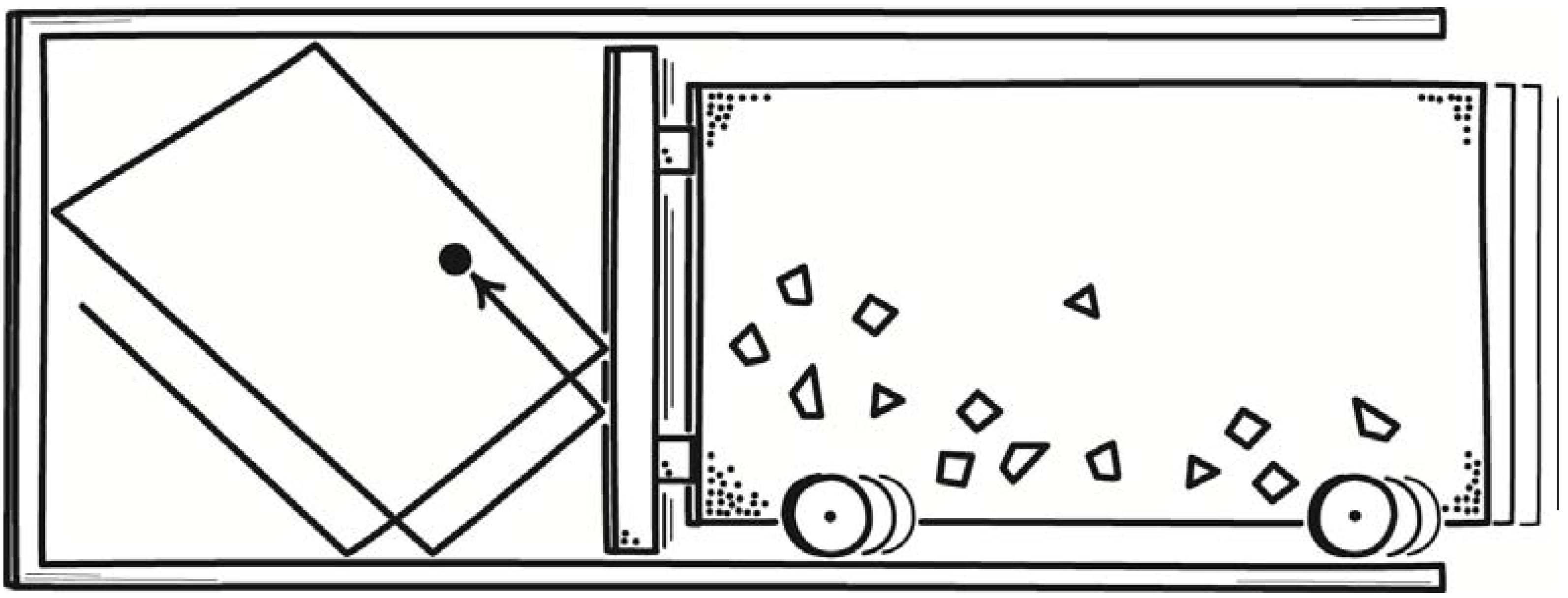
The massive body has one degree of freedom; it can move back and forth in the direction of the compression of the gas only. When it is at thermal equilibrium, its states are distributed canonically. That is, the probability that it is in a state with energy E, is proportional to exp(−E/kT). The energy is all kinetic, expressed as E = mv2/2, for m the mass of the body and v its velocity. It follows immediately that this velocity v conforms to a one dimensional Maxwell velocity distribution:
Since the velocity v in this distribution spans all positive and negative values, it follows that the mean velocity is zero and its variance is kT/m. (Since (12) is also a normal distribution, the mean and variance can be read directly from the formula. The variance conforms with the equipartition theorem, which requires the mean of the kinetic energy mv2/2 to equal kT/2. From this, we infer that the mean of v2 = (2/m).(kT/2) = kT/m).
The variance is just the expectation of v2. Hence we arrive at an estimate of the typical speeds of the mass when it is in a thermal equilibrium state, its “root mean square” velocity:
For a one kilogram mass at 25 C, we have vrms = 6.415 × 10⁻¹¹ m/s. (Computed using T = 273 + 25 = 298K and k = 1.381 × 10⁻²³ J/K.)This is a very small velocity. More pertinently, the body’s velocity will be fluctuating to and fro, around the mean value of zero. Hence if we bring the gas and the body arbitrarily close to their equilibrium conditions, we do not have a process in which the gas is inexorably compressed by the inertia of the moving mass. We just have two bodies fluctuating back and forth, with the extent of the massive body’s fluctuation macroscopically indiscernible.
To bring about a compression, we would need to drive the massive body away from its equilibrium state to one in which it can maintain a unidirectional velocity. This velocity must be faster than the rms velocity, for when the body moves with velocities of the rms size, interactions with the thermal environment will produce fluctuations that reverse unidirectional motion. We might just give the body a slight push to higher speeds, out of the thermal range where fluctuations will reverse the motion. Or we might incline the surface so that the mass slides down into a potential well. These are dissipative processes that would create thermodynamic entropy.
An early version of this problem appears in Szilard’s [12] introduction of the one-molecule engine thought experiment. He writes [12] (pp. 122–123) of the piston during the expansion of a one-molecule gas: “It is best to image the mass of the piston as large and its speed sufficiently great, so that the thermal agitation of the piston at the temperature in question can be neglected.” Szilard’s analysis depends on careful accounting of all changes in entropy. Inclusion of a piston in a non-equilibrium state compromises the accountancy, since it neglects the entropy created in driving the piston to this non-equilibrium state.
8. How to Compute Thermal Fluctuations
8.1. Fluctuations in Isolated Systems
The techniques used to compute thermal fluctuations in the no-go result require only elementary notions. The simplest case involves thermal fluctuations within an isolated system. Such a system is microcanonically distributed over its phase space. That means that every state is equally likely, so that the probability of the system being in some specific region of the phase space is proportional to the region’s volume. As we saw in Section 4, for macroscopic systems, the equilibrium state occupies virtually all the phase space. Macroscopically distinguishable non-equilibrium states occupy only a minute portion. The key assumption is an adaptation of relative occupation times to the probability distribution: the system point moves through the phase space so that the time spent in the various regions conforms to the uniform distribution of the microcanonical distribution. It spends time in a region in proportion to its volume, with very little of it in the small volume, non-equilibrium states. Figure 8 illustrates the time evolution of the system point over the regions.
This account is correct, but abstract and somewhat distant from physical cases. The striking and informative illustration is given by Einstein [37] in Section 5 of his celebrated light quantum paper. If we have an ideal gas of n molecules, what is the probability that a fluctuation will spontaneously compress the gas to half its volume? Since there is a probability of 1/2 that each of the independently moving molecules will happen to be is the designated half, the probability that all n will be found in it is just (1/2)n. Hence, the equilibrium uniform distribution of the gas occupies virtually all of the phase space. The spontaneously compressed state occupies merely a (1/2)n fractional part of the phase space, where this fraction will be exceedingly small for the macroscopic case, in which n is of the order of Avogadro’s number, 6.02 × 10²³. Hence the fluctuation will be exceeding rare.
Figure 8.
Time evolution of system point in phase space.

Einstein redescribes the probabilities in a way that is now standard. He employs “Boltzmann’s Principle,” which asserts informally that “Entropy = k log (probability)” to arrive at an expression for the entropy change in a fluctuation process between the equilibrium state “1” and the fluctuation state “2” of the spontaneously compressed gas:
S2 − S1 = k ln (1/2)n = −nk ln 2
This equation must be read cautiously. Traditional thermodynamics is a theory of equilibrium states and assigns thermodynamic entropy S to equilibrium states only. The quantity S1 conforms with this. It is the entropy of the gas equilibrium state. The quantity S2 does not conform, for it is assigned to a highly non-equilibrium state. A gas that has spontaneously compressed to half its volume will retain that state only momentarily before explosively expanding. To make sense of Einstein’s relation (14) we imagine it as telling us what the thermodynamic entropy of state “2” would be, were we somehow to trap it in its fluctuation state and keep it there, as a new, equilibrium state. We might, for example, insert a partition at the moment the spontaneous compression is complete, trapping the gas in its compressed state. Then the equation would be asserting a familiar result of elementary thermodynamics: an n molecule ideal gas compressed to half its volume has a decrease of nk ln 2 in thermodynamic entropy.
In short, the thermodynamic entropy S2 associated with the fluctuation state is really a means of describing the state in familiar macroscopic, equilibrium terms; it is the entropy the state would have, were it to be an equilibrium state. We can also restate Boltzmann’s Principle as relating the entropy of a state, equilibrium or otherwise, to the volume V of the phase space of the state:
S = k ln V
Read this way, the principle has become a definition of the thermodynamic entropy of non-equilibrium states.
8.2. Fluctuations in Isothermal Systems
The no-go result pertains to isothermal systems; that is, to systems in thermal surroundings of constant temperature with which they exchange heat. It turns out that the analysis of Section 8.1 of fluctuations in isolated systems can be carried over in its entirety, with two substitutions: thermodynamic entropy S is replaced by free energy F and phase volume V is replace by the partition integral Z(V) over V.
The isothermal system described is canonically distributed over its phase space. That means that the probability of each phase space point with canonical coordinates (x,π) is proportional to exp(−E(x,π)/kT). Hence the probability that the system will be found in some volume V of the phase space is determined by integrating this factor over V, forming the partition integral:
We can still use Figure 8 as a representation of the time evolution of the system, where the figure now only shows the portion of phase space associated with the system. The equilibrium state will still occupy virtually all of the phase space of the system. However now the time that the system point spends in each state will not be proportional to its phase volume V, but to the partition integral Z(V).
For equilibrium systems, the free energy F = U − TS is related to the partition integral by:
F = −kT ln Z
This equation is the analog of Boltzmann’s Principle (15) and should be read in the same way. When Z(V) is formed for a non-equilibrium state, the relation has become a definition. It defines the free energy F associated with the state as the free energy the state would have were it somehow trapped in its fluctuation and kept there as an equilibrium state.
Equation (17) can be inverted to return the rule that relates fluctuation probabilities for different states. The probability p of a state occupying phase volume V is proportional to the partition integral Z(V). (In the application that follows, the volumes V are drawn from a one-parameter family with the parameter λ, so that p is a density over λ.) Hence we have:
where the free energies of non-equilibrium states are introduced by definition through (17) above using the partition integral Z(V) over their phase volumes V.
9. The No-go Result
9.1. Instability of Self-Contained, Isothermal, Thermodynamically Reversible Processes
Consider an isothermal, thermodynamically reversible process consisting of n component systems exchanging work and in thermal contact with the environment. The process is self-contained. That means that the component systems may exchange heat and work with each other, but exchange of heat is the only interaction with the environment. The thermodynamically reversible process consists of a sequence of equilibrium states, accessible to one another, parametrized by λ. Our goal is to move the process from the initial state λ = λinit to the final state λ = λfin. Absent fluctuations, we would drive the process forward by the slightest possible disequilibrium that would allow the process to proceed from start to end with arbitrary slowness.
That arbitrarily slow driving is no longer possible, however, for molecular-scale systems, when we allow for fluctuations. For the states comprising the process must be accessible to one another and fluctuations will drive the system back and forth wildly in behavior that generalizes the wild motions of the piston in the one-molecule gas expansion of Section 5 above. To see this we recall two results. From Section 8, Equation (18), we have that the probabilities densities p(λ1) and p(λ2) that the system is driven by fluctuations to be at stage λ1 or λ2, satisfy:
For a thermodynamically reversible process in which the thermodynamic entropy of the total system remains constant, we have from (11) in Section 6 that the sum of the component system free energies is constant, so that:
whatever the values of λ1 and λ2. It follows that:
F(λ1) = F(λ2)
(“No-go”) p(λinit) = p(λ1) = p(λ2) = p(λfin) p(λ) = constant, all λ
This uniformity of probability has changed the character of a thermodynamically reversible process. Without fluctuations, the system will remain stably in each of the equilibrium states comprising the process. There is no imbalance of generalized forces to move the system from one equilibrium state to another. When fluctuations are added, they provide the mechanism that will move the system spontaneously from one state to another.
This motion can be described thermodynamically. The system, released from confinement in some subregion of the λ space, expands irreversibly in the thermodynamic sense to a new state that occupies the full λ space. Assume that the initial state is confined to a 1/n th portion of the full λ space. Since the probability distribution is uniform over the full λ space, the partition function Zinit is 1/n th the size of the full space partition function Z. That is Z = nZinit. Since free energy F = −kT ln Z by (17), we have for the free energy change during the motion that:
ΔF = −(kT ln Z − kT ln Zinit) = −kT ln n
Using (11), we have the entropy and free energy changes during this expansion:
ΔStot = k ln n = −ΔFsys/T
The thermodynamics is analogous to the uncontrolled n-fold expansion of a one-molecule gas, which also creates k ln n of thermodynamic entropy.
The constancy of the probability density of (20) represents a distribution associated with the new dynamic equilibrium state in which the system moves freely over the states indexed by λ. What the relation does not show is the time scale over which the expansion occurs and the new equilibrium is established. We have very different behavior on the molecular and macroscopic scale.
For molecular-scale systems, the equilibrium will be established very rapidly. Fluctuations are large and rapid in relation to the distance and time scales of molecular systems. (see Section 10.1 for an illustration.) If we were somehow able to set up the system at any particular stage λ of the process, fluctuations would immediately move it to other stages, with all stages having equal probability. If the system happens to be somewhere near the start of the process, it is equally likely that it will remain there or be flung to the end state. If the system happens to be somewhere near the end of the process, it is equally likely that it will remain there or be flung back to the start.
The original notion of a thermodynamically reversible process was of quiescent equilibrium states; or, more precisely, a very slow transition through them driven by the gentlest of nudges, supplied by very slight deviations from equilibrium. That is no longer possible. The arbitrarily slow progress imagined is obscured behind the wild gyrations of fluctuations.
If we move to the macroscopic scale, the result (20) still obtains. However the difference of time scales intervenes. While any macroscopic equilibrium state in the process will be driven by fluctuations to the dynamical equilibrium of (20), the fluctuations are so miniscule that the extremely slow shift toward the dynamical equilibrium is invisible to us as macroscopic observers.
9.2. What It Takes to Overcome Fluctuations
Self-contained, isothermal, thermodynamically reversible processes are impossible at molecular scales. However we can overcome the fluctuations and get a process to proceed from its initial to its final stage if we are prepared to admit some irreversibility; that is, if we are willing to create thermodynamic entropy. Completion of the process will be achievable only probabilistically. However the probability of completion can be made arbitrarily high, if we are willing to create enough thermodynamic entropy.
We can use the relations of Section 6 to estimate the minimum thermodynamic entropy creation needed to enforce each chosen probability of successful completion. Relation (18)/(19) tells us that a sufficiently large decrease in free energy over the process can provide any chosen probability gradient. Let us say that our initial state “init” occupies a small interval λ = λinit to λinit + δλ; and our final state “fin” occupies an interval of the same size λ = λfin − δλ to λfin. We set up our initial state so that it is confined to the indicated interval. It is an equilibrium state that has free energy Finit. We release it so that the process can begin. The system state expands to fill the λ space. There will be some small probability Pinit that fluctuations will carry the system back to its initial state (note: Pinit is not the probability that the system starts in the initial state, but that fluctuations carry the system back to it). There will be a larger probability Pfin that the system will move down the free energy gradient into the final state. If the free energy gradient across the space is sufficiently large, in the new dynamical equilibrium, the system will end up with arbitrarily high probability in the final state. We now trap it in some way in that final state so that it reverts to an equilibrium state. The free energy of that state is Ffin. Relation (18)/(19) enable us to compute:
where ΔFsys = Ffin − Finit and ΔStot is the total thermodynamic entropy change of the entire system and surroundings during the process. Relation (11) TΔStot = −ΔFsys has been used for the last equality. (Since the free energy and entropy changes are computed between equilibrium states, these quantities have their normal meanings.)
The expression (22) for the ratio Pfin/Pinit does not give us a direct measure of the value of Pfin attainable through creation of some definite amount of thermodynamic entropy ΔStot. For Pfin and Pinit are related by the inequality Pfin ≤ (1 − Pinit). If stages other than the initial and final have non-negligible probability, the relation is a strict inequality and Pfin has less than its maximum value. We arrive at the maximum probability Pfin for a definite entropy creation, if we assume that the free energies of all stages other than the initial and final have been so elevated that the probabilities of these stages have become negligible. For this least dissipative case, we have:
where Ofin is the odds ratio for achieving the final stage.
Pinit + Pfin = 1 Ofin = Pfin/(1 − Pfin) = Pfin/Pinit
Inverting (22) gives the minimum thermodynamic entropy ΔStot that must be created to enforce an odds ratio Ofin favoring completion:
ΔStot = k ln Ofin = −ΔFsys/T
The minimum will not be achievable typically since it requires the free energies in the process to be so contrived that only the initial and final stages have non-negligible probabilities. (see Section 10.3 below for an illustration of how this may be achieved).
This minimum thermodynamic entropy creation is independent of temperature. Hence cooling the system to low temperatures will not avoid dissipation; at best it will slow down the disruption of fluctuations. Relation (23) reports the minimum thermodynamic entropy creation required for each completed step. If our process is complex and requires many steps to be chained together, with each completed before the next starts, then we must create at least this much thermodynamic entropy for each step.
Computing a few cases gives a sense of the quantities of thermodynamic entropy that must be created to overcome fluctuations:
For Pfin = 0.95 and odds ratio Ofin = 20, ΔStot = k ln 20 = 3k; ΔFsys = −3kT
An odds ratio of 20:1 is quite modest and usable only if we are chaining few processes together. However it requires entropy creation of 3k and that exceeds the k ln 2 = 0.69k of thermodynamic entropy tracked by Landauer’s principle. If we want a strong assurance of completion, might choose:
For Ofin = 7.2 × 10¹⁰, ΔStot = 25k; ΔFsys = −25kT
While this is a high odds ratio and creates a large amount of thermodynamic entropy on a molecular scale, it is a negligible amount macroscopically. The corresponding thermal energy, 25kT, is just the mean thermal energy of ten oxygen molecules.
Hence, the quantities of entropy needed to overcome fluctuations on the molecular scale are large, but negligible on the macroscopic scale. On the latter scale only, we may continue to think of thermodynamically reversible processes as approachable arbitrarily closely by sufficient reduction of disequilibria.
10. Simplest Illustration of the No-go Result: Bead on a Wire
10.1. The Undriven Bead
The simplest illustration of the no-go result is provided by a bead that can slide frictionlessly along a horizontal wire. In macroscopic thermodynamics, without fluctuations, the bead at rest on the wire is an equilibrium thermodynamic system, albeit an extremely simple one. The sequence of positions it may occupy along the wire is a sequence of equilibrium states that comprises a thermodynamically reversible process. Since all forces are in perfect balance, nothing drives the bead forward from one state to the next. We provide the slightest disequilibrium needed merely by tilting the wire minutely from the horizontal, so that the bead now slides, arbitrarily slowly, down the wire.
The process becomes more interesting if we consider fluctuations. The bead is a thermal system undergoing fluctuation motions, akin to Brownian motion, as shown in Figure 9. As a result, even when the wire is perfectly horizontal so that there is no imbalance of forces, the fluctuations will carry the bead to neighboring equilibrium states. The bead’s motion will expand to a new dynamical state in which it traverses the full width of the wire.
Figure 9.
Bead a Wire.

The magnitude of this effect is scale dependent. To see this, note that the velocity of the bead is given by the one dimensional Maxwell distribution (12) with typical speeds given by the root mean square velocity (13); that is, , where m is the bead’s mass.
Consider a macroscopically sized bead of 5 g on a one-meter wire:
For m = 5 g and T = 25 C, vrms = 9.071 × 10⁻¹⁰ m/s
This is a very slow speed, covering only molecular-scale distances in each second. If the bead could maintain this velocity in one direction, it would take 35 years to cover a wire of one-meter span. Of course it cannot maintain the motion unidirectionally, since the bead is constantly changing direction. While the bead is undergoing the irreversible expansion indicated in the no-go result, the process advances so slowly as to be invisible on macroscopic scales.
Now consider a bead of a molecular-scale size. The molecule n-heptane C7O16 has the round number atomic mass of 100 amu = 1.6605 × 10⁻²⁵ kg and is fairly large and heavy, compared to ordinary gases and liquids, such a CO2 and H2O molecules (the 100 is rounded down from the exact value of 100.2; n-heptane also has the distinction of being the component of gasoline that defines the zero point of the octane rating scale).
For m = 100 amu and T = 25 C, vrms = 157 m/s
With speeds of this order, the molecule, when released on the wire, will immediately adopt motions that span the full one-meter length of the wire. That is, the irreversible expansion driven by fluctuations will be completed rapidly.
10.2. The Driven Bead
Fluctuations will scatter a light, molecular-scale bead uniformly over the wire. These motions preclude a thermodynamically reversible process in which the bead moves very slowly across the wire, advancing quietly from equilibrium state to equilibrium state. We can overcome these fluctuations and force the bead to pass from one side to the other by introducing a disequilibrium that creates thermodynamic entropy. The simplest way to attempt this is to tilt the wire, so that an unbalanced gravitational force overcomes fluctuations and draws the bead to the desired end.
This arrangement is shown in Figure 10, where the wire of length L is inclined at angle θ to the horizontal. Progress along the wire is parameterized by distance λ, where λ varies from 0 to n. The initial state is λ = 0 to 1 and the desired end state is λ = n − 1 to n. The bead’s Hamiltonian is:
where:
is the energy gradient per unit λ. The partition integral for the portion of the wire between λ1 and λ2 is:
H = (1/2)mv2 − mgL sinθ λ/n = (1/2)mv2 − ελ
ε = (mgL sinθ)/n
Figure 10.
Gravity driven bead on a wire.
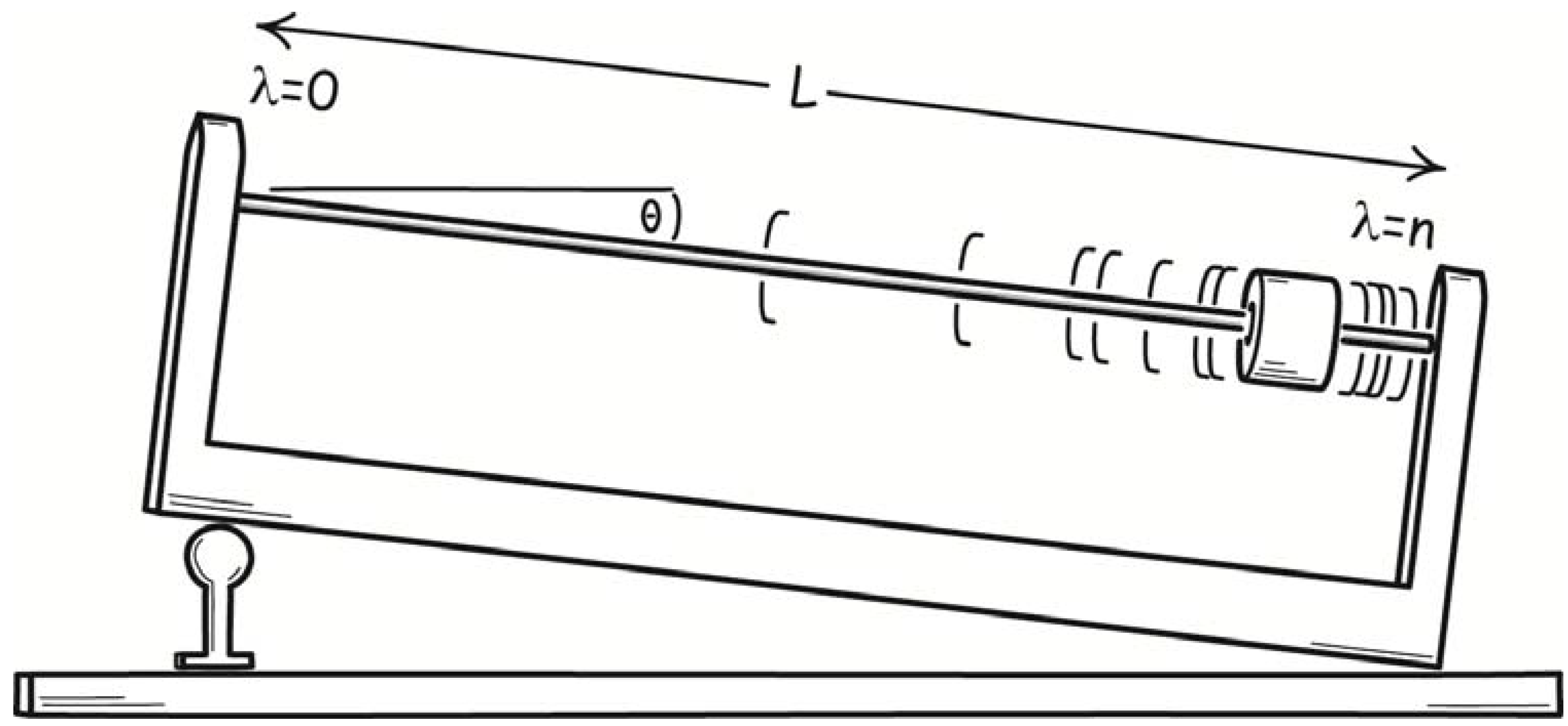
The canonical coordinates are λ for the configuration space and π = mv for momentum space. The contribution of the momentum degree of freedom is written as M and is not computed since it plays no role in the ensuring calculation.
The probability that the released bead is in the desired end state λ = n − 1 to n is:
This expression has two limiting cases. When the energy gradient is small, that is ε/kT << 1, we have:
Then the energy gradient is negligible and the bead position is uniformly distributed over the λ space. However, if the energy gradient is steep so that εn/kT >> 1 and exp(−εn/kT) ≈ 0, then Pfin ≈ 1 − exp(−ε/kT). Inverting we find:
if we write 1 − Pfin = 10−m.
ε/kT = −ln (1 − Pfin) = m ln (10) = 2.3026m
The total thermodynamic entropy created in the release of the bead is given through (11) and (17) as:
Once again this expression has two limits. When the energy gradient is small, that is ε/kT << 1, we have:
ΔStot = k ln n
It is simply the total thermodynamic entropy created when the bead-gas undergoes an irreversible n-fold expansion. If ε/kT >> 1, then expression (29) simplifies to:
ΔStot = ε(n − 1)/T
This expression is easily interpreted. When ε/kT is large, the energy gradient is steep and the bead released from the initial state λ = 0 to 1 almost certainly falls down to the final state λ = n − 1 to n. In falling, it loses potential energy of ε per unit of λ, which amounts to ε(n − 1) overall. This energy is passed to the surroundings as heat and results in an increase of total thermodynamic entropy of ε(n − 1)/T. (Note that this conclusion cannot derive directly from the Clausius definition that ΔS = qrev/T since the process is not a thermodynamically reversible process.) We can relate this entropy creation to the odds ratio Ofin by combining (28) and (31) to recover:
where the last approximation holds for Pfin close to unity.
ΔStot = ε(n − 1)/T = k(n − 1) ln (1/(1 − Pfin)) ≈ k(n − 1) ln Ofin
10.3. The Least Dissipative Driven Bead
This quantity (32) of entropy creation is well in excess of the minimum needed, k ln Ofin, as shown in (23). It exceeds it by a factor of (n − 1). The minimum is achieved by rendering all intermediate stages probabilistically inaccessible. The assumption of the inaccessibility of these intermediate stages enabled us to pass from the relation (22) on Pfin and Pinit to the minimum entropy relation (23). For the bead on the inclined wire, the n−2 intermediate stages are all accessible and their accessibility is responsible for the factor of (n − 1) in (32).
To arrive at the least dissipative case of (23), instead of inclining the wire, we would bend it so that the intermediate stages are elevated. Now the bead must pass over a probabilistically-hard-to-ascend mountain. It then falls into the probabilistically-favored energy well of the final state at the end of the wire, much lower in the gravitational field, as shown in Figure 11.
The effect of this mountain is to make negligible the probability that the bead is in the stages intermediate between the initial and final stages. Hence we have:
so that we have for the odds of achieving the final state:
Pinit + Pfin ≈ 1
Figure 11.
The least dissipative driven bead.
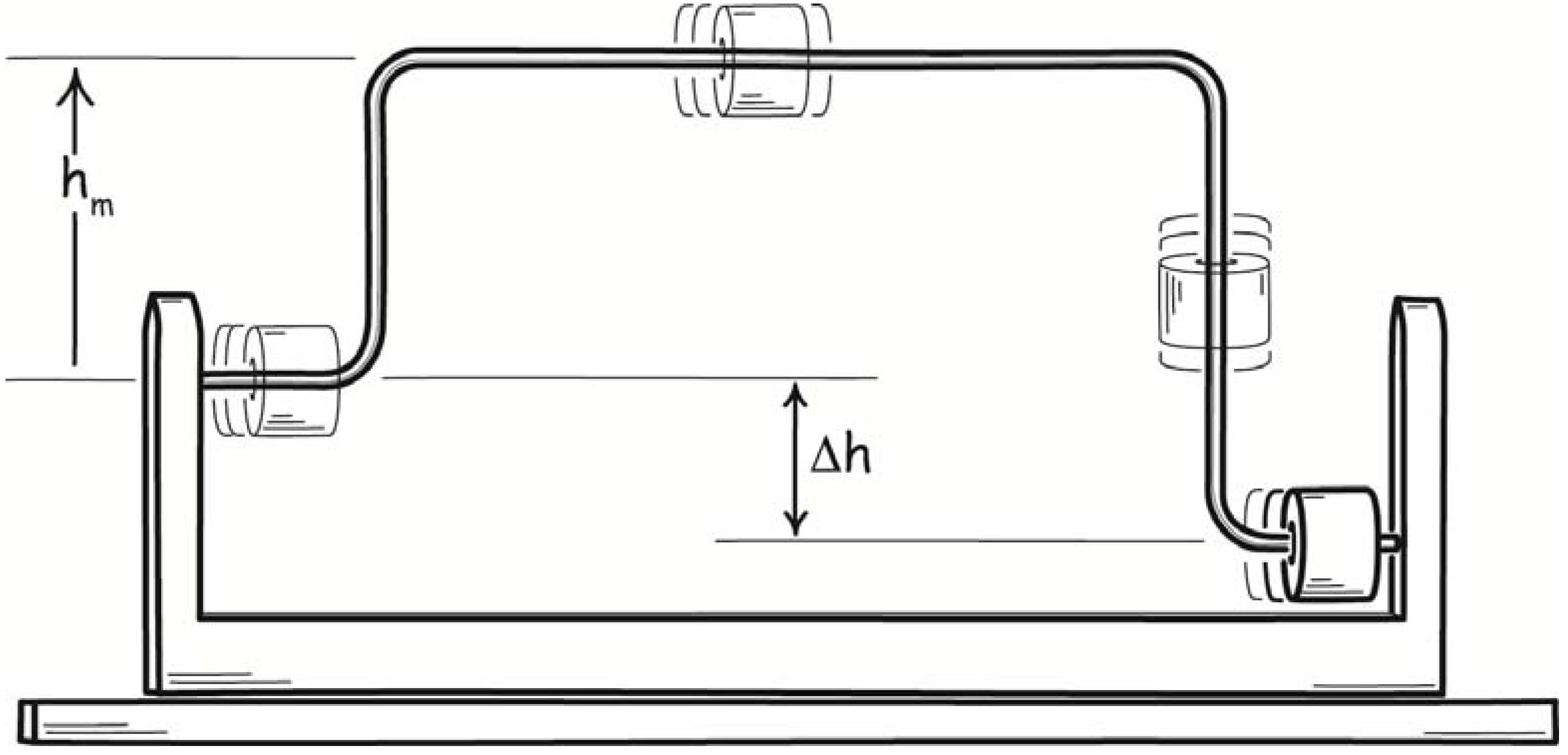
The probability of intermediate stages can never be zero exactly, else the bead would be unable to pass through the intermediate stages and complete the process. As long as the wire is elevated to some finite height hm where the bead will have energy E(hm) = mghm, the bead will always be able to ascend; for the probability that it rises to height hm is proportional to exp(−E(hm)/kT) = exp(−mghm/kT). However, as hm becomes large this probability factor will become exponentially small. This smallness will not prevent the bead passing over the intermediate stages. Rather it will greatly slow the passage. We must wait for an improbable energy fluctuation large enough to fling the bead up the mountain.
If the positive-valued difference in elevation of the initial and final parts of the wire is Δh, then the (ordinary) energy change between them is ΔE = −mgΔh for the bead. If the initial state corresponds to distance along the wire λ = 0 to 1 and the final state to λ = n − 1 to n as before, then we have:
where the last equality uses (11). Then we have for the odds of achieving the final state:
Inverting to recover ΔStot, the resulting expression approximates the minimum entropy creation ΔStot = k ln Ofin of (23).
Since rendering the probability of intermediate stages negligible requires considerable contrivance, we revert in the next section to the simpler arrangement of Section 10.2 of the bead driven by a uniform incline.
10.4. The Driven Bead at Molecular and Macroscopic Scales
The one set of results in Section 10.2 for the driven bead have very different imports at the molecular and macroscopic scales. To see this, we compute the angle θ needed to enforce completion of the process with a probability of success of Pfin = 0.999, so that m = 3. From (28) for T = 25 C = 298 K, we have that:
ε = kT (2.3026)m =2.842 × 10⁻²⁰ J
For a one meter wire (L = 1m), 5 g = 0.005 kg mass and n = 10, we have:
ε = (mgL sinθ)/n = 0.004903 sinθ J
Solving these last two equations for θ we find:
θ ≈ sin θ = 2.842 × 10⁻²⁰/0.004903 = 5.796 × 10⁻¹⁸ radians
This is a very small angle. Since it is located at the end of radial arm of one meter, it means that the destination end of the wire is depressed by 5.796 × 10⁻¹⁸ m. To get a sense of just how small that is, recall that the Bohr radius of a hydrogen atom is 5.29 × 10⁻¹¹ m. The depression of the end of the wire is seven orders of magnitude smaller!
This astonishing result expresses quite clearly how little fluctuations matter as we seek to implement thermodynamically reversible processes on macroscopic scales. We approach thermodynamic reversibility by making the angle of deflection θ closer to zero. Even when our deflection is merely at atomic distances, we are still many orders of magnitude away from the domain in which fluctuations would matter.
Things are quite different, however, if we consider a molecular-scale bead of 100 amu. We will start with the maximum deflection possible, θ = π/2, sin θ = 1, so that the wire is vertical. Then, with n = 10, we have:
ε = mgL/n = 1.6284 × 10⁻²⁵ J
This is five orders of magnitude smaller than the value of ε needed to enforce completion of the process, the 2.842 × 10⁻²⁰ J computed above.
For this case, we have ε/kT = 0.00003958. Hence the small ε/kT limit results (27) and (30) apply. The small bead motions, upon its release, expand to a dynamical state that uniformly fills the vertically-oriented wire.
In retrospect, this behavior is not surprising. n-heptane is a volatile liquid at 25 C and its molecular mass is 100 amu. All we are seeing is that its molecular motions are sufficiently vigorous at ordinary temperatures to overcome gravity and form a dilute vapor that will uniformly fill a space. These molecular motions, however, are the same as the fluctuation motions that disrupt efforts to realize thermodynamically reversible processes. The contrast between the macroscopic and microscopic scales is stark. On the macroscopic scale, fluctuation phenomena are indiscernible. On the molecular scale, they give matter some of its most familiar physical properties.
For completeness, from (32) and (28), the thermodynamic entropy created in the case of the 5 g bead for n = 10 is k(n − 1)m(2.3026) = 62.2 k. From (30), the thermodynamic entropy created in the release of the 100 amu bead for n = 10 is k ln 9 = 2.197 k. The first entropy creation is significantly larger since the process recompresses the bead location to the final state, by a less efficient means.
11. Moving a Charge through a Channel
The illustrations so far have been of simple mechanical systems: one-molecule gases and beads on wires. In this section and the following, we shall see two electrical examples. The basic physics of the examples is essentially similar to the cases already seen. There are balances of generalized forces, transfers of heat and the compression and expansion of phase spaces, but this time electrical degrees of freedom are engaged.
One of the simplest processes in a molecular-scale electronic computer is the moving of a single charge through a conducting channel, as shown in Figure 12. It is an elementary means of communication between components.
Figure 12.
Charge in a channel.
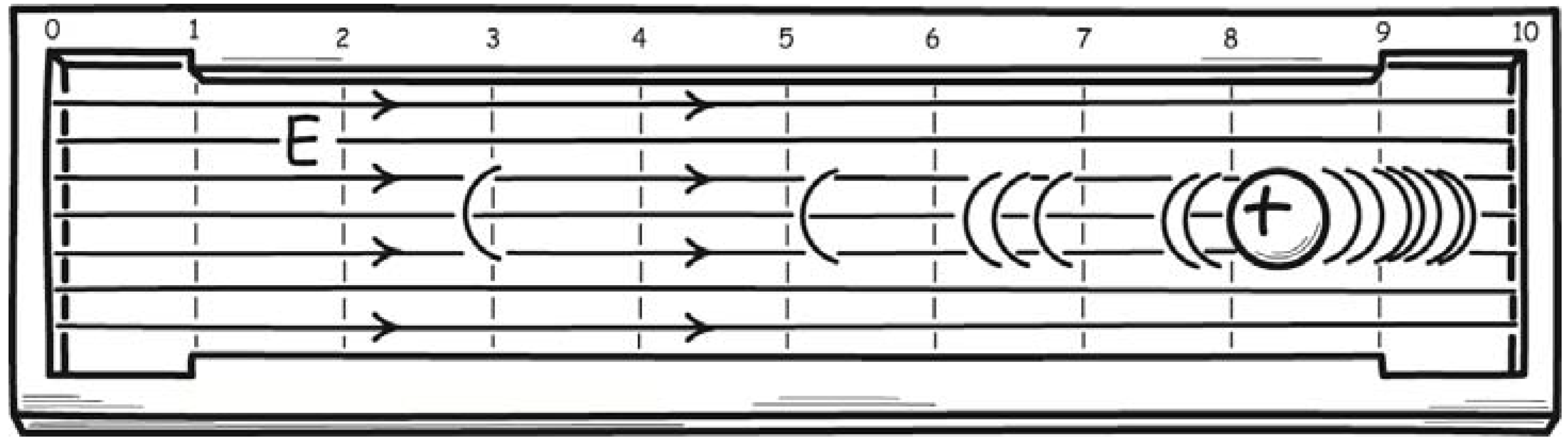
If left to itself, thermal fluctuations will scatter the charge with uniform probability over the length of the channel, so that passage of the charge through the channel is not assured. An electric field E is applied to enforce the charge’s motion from the initial position λ = 0 to 1 to the final position λ = n − 1 to n. Since the field is confined to a linear channel, its lines of force do not diverge and the field E is constant. As a result, the Hamiltonian of the charge has the same λ dependence as that of the bead on the wire:
where, in this case, the energy gradient ε per unit λ is due to the constant field E acting on the charge q over the channel length L:
Hmom is the contribution of the momentum degrees of freedom of the charge and is not computed, since it plays no role in calculations to follow. Otherwise, the analysis of the charge in the channel is essentially similar to that of the bead on a wire; and the relations derived for the bead can be applied to the charge.
H = Hmom − ελ
ε = EqL/n
At equilibrium, the charge is distributed canonically over the length of the channel with a probability density proportion to exp(−H/kT), that is, as:
where the distribution is normalized by Z = (kT/ε)[exp(εn/kT) − 1]. The effect of increasing the field strength E is shown in Figure 13 for the case of n = 10.
p(λ) = exp(ελ/kT)/Z
Figure 13.
Charge position probability distribution.
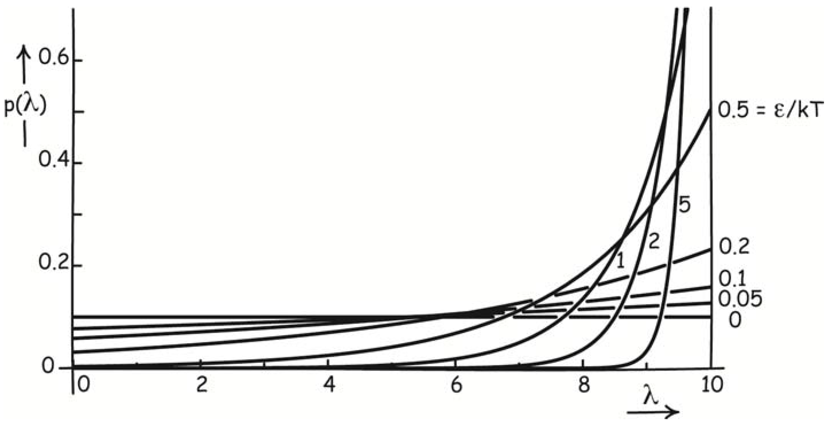
For small E, so that ε/kT << 1, the charge position is roughly uniformly distributed over the channel. As the field E increases in strength, the charge position is localized towards the intended destination, λ = 9 to 10, with near complete localization achieved by ε/kT = 5.
Relations (26), (27) and (28) provide precise values for the probability Pfin that the charge is driven into the intended destination. Relation (32) gives the total entropy ΔStot created in the process. We read from them that:
For Pfin = 0.95; ε/kT = −ln 0.05 = 3; ΔStot = k(10-1) ln 20 = 27 k.
For Pfin = 0.99; ε/kT = −ln 0.01 = 4.6; ΔStot = k(10-1) ln 99 = 41 k.
For Pfin = 0.999; ε/kT = −ln 0.001 = 6.9; ΔStot = k(10-1) ln 999 = 62 k.
As before, these quantities of entropy creation exceed the minimum determined in (23) by a factor of (n−1) = 9. The excess results from the accessibility of the intermediate positions in the channel from λ = 1 to λ = 9. Entropy creation could be reduced by employing an inhomogeneous field that makes these intermediate positions probabilistically less accessible.
This simple illustration shows that entropy created to overcome thermal fluctuations will have a controlling influence in molecular-scale electronic computational devices. The illustration neglects further, significant sources of thermal fluctuations. The electric field has been taken as fixed. It is not. The electromagnetic field is a thermal system in its own right and, as a result, undergoes thermal fluctuations, commonly treated as Johnson-Nyquist noise.
It turns out that the channel manifests one of the simplest cases of Johnson-Nyquist noise. The electric field in the channel must be maintained by electric charges. As a result, the channel is really the interior of a capacitor with voltage V = EL. The energy of a capacitor of capacitance C is CV2/2. Hence its Hamiltonian is quadratic in V and the equipartition theorem assigns a mean thermal energy of kT/2 to it. Thus an otherwise uncharged capacitor will acquire a mean energy CV2/2 = kT/2 due to thermal fluctuations. So we can expect root mean square fluctuations in its voltage of . A more complete analysis of the system would need to accommodate these fluctuations.
12. Measurement: Compression of a Dipole Phase Space
After Szilard introduced information-theoretic considerations into the exorcism of Maxwell’s demon, a new consensus developed: the demon must fail to reverse the second law of thermodynamics because of an inevitable entropic cost that arises in measurement processes. Successful operation of the Szilard one-molecule engine described in Section 3.1 requires the demon to locate the position of the trapped molecule, so that the piston-weight system can be introduced in a way that allows expansion in the appropriate direction. The measurement operation that acquires that one bit of information, it was decided, must create k ln 2 of thermodynamic entropy and creation of just that amount was all that was needed to protect the second law from violation.
This earlier consensus was supplanted by the newer view that draws on Landauer’s principle and identifies memory erasure operations are the real locus of dissipation in the demon’s functioning. (Section 2 of Earman and Norton [23] provides a brief review of the change of consensus.) This new consensus needed to reverse the earlier assertions by von Neumann, Brilllouin, Gabor and others (as outlined in [23]) that measurement was the locus of dissipation. For, in the new view, erasure is the unavoidably dissipative step and no other. The new view needed to establish that measurements could be made on molecular-scale systems by thermodynamically reversible processes. A demonstration of this possibility was provided in proposals for measuring operations that, it was asserted, could be implemented by molecular-scale, thermodynamically reversible processes (for example, see Bennett [16] (Section 5) and Bennett [17] (p. 114) and Norton [24] (Section 7.3) for my response). Since these processes must go to completion, it is now clear that all such proposals have to be defective, for they contradict the no-go result above. The analysis of the proposals must at some point neglect consideration of relevant thermal processes; and, typically, it is the thermal properties of the “driver” in the general description below.
To begin with, a measurement operation involves two components. There is a target system, one of whose properties is to be measured; and a detector that will be coupled with the target system and adopt a state that reflects the target system property. Thermodynamically, the measurement operation is a compression of the phase space of the detector. The detector starts in a neutral state in which it moves freely between the various possible final states. The coupling with the target system compresses the range of motion down to the state that reflects the target system property.
The compression must result from the application of a generalized thermodynamic force to the detector. That force is typically derived from a third component, a “driver,” that brings the detector into interaction with the target system. If the measurement is to be self-contained and thermodynamically reversible, then the force applied by the driver must be in perfect balance with the detector’s resistance to compression. The result will be a process whose total free energy—that of the detector, target and driver combined—is constant. The no-go result then asserts that fluctuations will scatter the combined system state over the entire range of the measurement process. A thermodynamic entropy creating disequilibrium must be introduced to overcome the fluctuations, with a minimum entropy creation of Equation (23).
A concrete example of measurement is provided by a system for measuring the sign of an electric charge that comprises the target system. The sign is detected by an electric dipole that approaches the charge and aligns itself with the electric field of the target charge, thereby revealing the sign of the charge. We shall see that the attractive force of the charge on the dipole provides more than enough force to pull the dipole towards it. One normally discounts the force between a charge and a dipole since it dilutes with the inverse cube of distance. However, in this case, it is of decisive importance. In fact, it turns out to be so strong that a third component is needed to restrain it if we are to keep all generalized thermodynamic forces in perfect balance. In effect, to a large degree, the driver is built into the attractive force between the target charge and the measuring dipole.
The arrangement is shown in Figure 14. The detector is a dipole that is free to turn between two positions, parallel and anti-parallel to the electric field of the target charge. For concreteness, the target charge is set to be positive. The positive “+” state of the dipole points away from the charge; the negative “−” state points towards the charge. In its initial state, the dipole can move freely between both + and − states. To simplify the analysis, we assume that all intermediate states between + and − are energetically disfavored by some hidden mechanism, so that they need not be considered. It is a two state device. When it is remote from the target charge, the dipole state moves freely by thermal agitation between the + and − states. As it is lowered into the electric field of the charge, the + state becomes energetically favored, its phase space is compressed and the dipole adopts a state that provides the outcome of the measurement. Further processes, not shown, would be needed to lock in the outcome state and recover it for use elsewhere.
Figure 14.
A dipole measures the sign of a charge.
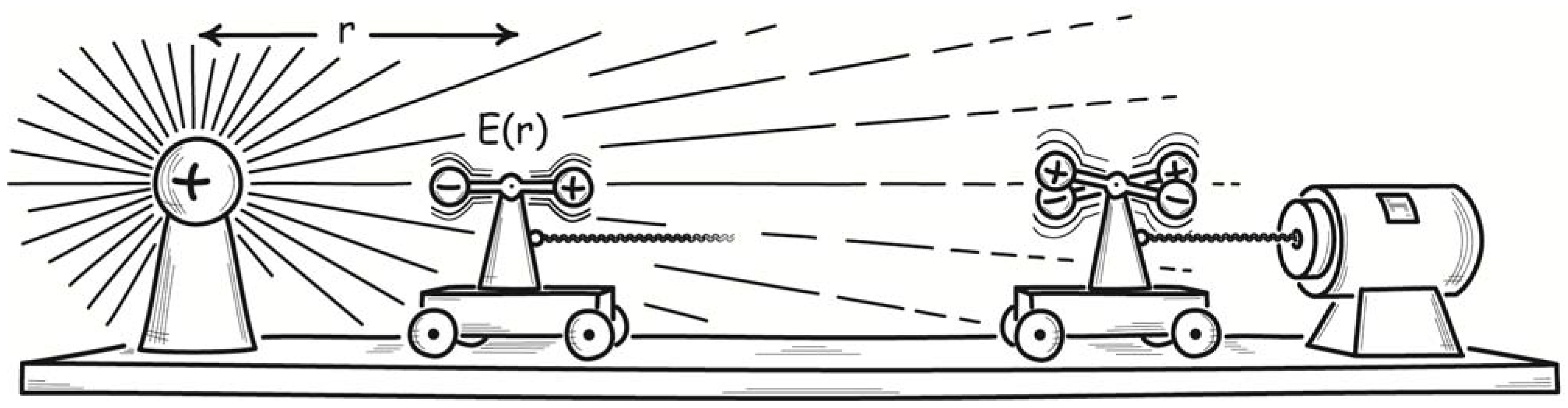
The dipole has an electric dipole moment p. When it is r distant from the charge, it is immersed in the electric field E(r) of the charge and has energies –E(r)p and E(r)p according to whether the dipole moment is parallel to the E field (+) or antiparallel to it (−). The dipole partition integral is:
Z = MΩ [exp (E(r)p/kT) + exp(−E(r)p/kT)] = MΩ 2 cosh(E(r)p/kT)
When the dipole is in the + or – state, it is assumed that it has freedom to move through the very small angle Ω. This freedom is associated with momentum degrees of freedom that contribute the term M. It is not evaluated since it plays no role in the computations below.
The partition integrals, restricted to the states + and −, are:
Z+ = MΩ exp (E(r)p/kT) Z− = MΩ exp (−E(r)p/kT)
From these, we can compute the probability P+ = Z+/Z of a successful measurement and P− = Z−/Z of an unsuccessful measurement, if we manage to bring the dipole to a distance r from the target charge and hold it there so that equilibrium is established. The expression for the odds ratio O+ is simpler:
Inverting, we recover:
To preclude confusion: this odds ratio O+ is not the odds that we bring the dipole to position r. Rather, is the odds that, once we have the dipole stably at position r, the measurement has succeeded in returning the correct + value.
It follows from (37) that, at the start of the measurement process, when r is large and E(r) ≈ 0, we have O+ = 1, so that P+ = P− = 1/2. For O+ = 20, we have Ep/kT = 1.50; for O+ = 99, we have Ep/kT = 2.30. This Equation (37) tracks the extent of completion of the compression of the dipole space that arises as r decreases and the field E(r) surrounding the dipole increases. The dipole state is initially equally distributed across + and − states; and, during the measurement, it is compressed to the + state, as shown in Figure 15.
Figure 15.
Compression of the dipole phase space.

The thermodynamics of this compression is governed by the free energy F, mean energy U and thermodynamic entropy S of the dipole, or, more precisely, the interacting charge-dipole system. The free energy is:
FM is the contribution from the momentum degrees of freedom and is not computed, since it is constant through the processes considered here. The small angle Ω is here and henceforth silently absorbed into an additive constant that is not shown. The mean energy U(r) of the dipole is:
The thermodynamic entropy S(r) of the dipole is derived from (38) and (39) as:
The energy term UM and entropy term SM derive from the momentum degrees of freedom and are not computed.
The free energy F(r) is strictly decreasing as r diminishes and the dipole approaches the target charge. It follows that the interaction between the charge and dipole, as mediated by the electric field E(r), is attractive. There is a generalized force X(r) drawing the dipole towards the charge. We can compute the generalized force from (38) as:
During this process, it follows from (40) that the change in thermodynamic entropy of the dipole is:
for, when r is large so that E(r) ≈ 0, we have S(r) = SM + k ln 2; and for E(r)p/kT large, we have S(r) = SM. This reduction in entropy is just that associated with the compression of the dipole phase space from the two states + and − to the single state +. In the early stages of the process, the generalized force X(r) acts to compress the phase space of the dipole. However, once the dipole phase space is well compressed to the + state and E(r)p/kT is greater than 2 or 3, we have that tanh(E(r)p/kT) ≈ 1, so that X(r) reduces to:
ΔS(r) = −k ln 2
That is, the generalized force X(r) has become an ordinary force pulling a dipole, fixed in the + state, deeper into the charge’s field. It results from the fact that the dipole energy −E(r)p becomes more negative as it moves closer to the charge. There is no longer any resistance force arising from the compression of the dipole phase space.
If we simply release the dipole and let it fall freely towards the target charge, then the work to compress the dipole space is supplied fully by the attractive force of the target charge. Allowing the dipole to fall freely, however, is not a thermodynamically reversible process. In order to achieve thermodynamic reversibility, we would have to lower the dipole gently towards the target charge. The device that performs this lowering is shown in Figure 14. It must perform the delicate task of exactly counterbalancing the generalized force (41) that is drawing the dipole towards the charge. That is, the device must exert a generalized force Xdev(r) that satisfies:
X(r) + Xdev(r) = 0
Since X = −dF/dr, It follows that the free energy Fdev(r) of the device must satisfy:
where F(r) is the dipole free energy as given by (38). Hence we have the same expression for Fdev(r), with the crucial exception of a sign change:
F(r) + Fdev(r) = constant
The no-go result now applies: the system free energy is a constant over all the stages of the measurement process, so that fluctuations will scatter the system uniformly over them. As before, on these molecular scales, there are significant thermal fluctuations within the dipole-charge system; and there must also be significant fluctuations within the operation of a device delicate enough to be capable of delivering tiny molecular-scale forces. These fluctuations overwhelm the intended process.
If we are to bring the measurement process to completion, we must introduce some entropy-creating disequilibrium to overcome these fluctuations. One might think that the natural way to do this is to investigate the inner workings of the device and weaken some factor slightly. That would be a difficult task to do realistically. It turns out to be quite hard to devise a thermal system with the free energy (44) that uses familiar components.
Fortunately, we can dispense with the device entirely. For without it, merely releasing the dipole to fall towards the charge already introduces barely enough disequilibrium to ensure completion of the measuring process. To see this, take the initial stage of the process to be one for which r = rinit is sufficiently large so that E(rinit) ≈ 0. Then we have:
Finit = FM – kT ln 2
We take the final stage r = rfin to one for which E(rfin)p/kT is sufficiently large for 2 cosh(E(rfin)p/kT) = exp(E(rfin)/kT). Then we have:
Ffin = FM − E(rfin)p
It now follows that the free energy change is:
ΔF(rfin) = −(E(rfin)p − kT ln 2).
From (19), we have for the probability densities over r, p(rinit) and p(rfin), that fluctuations carry the system to either the initial or final state:
where (37) is used to introduce the odds O+ for a successful measurement, given that the dipole has arrived at position rfin.
Relation (46) tells us that selecting a value of rfin large enough to assure a successful measurement is not enough to overcome fluctuations. To see the problem, select some value of O+ that ensures a successful measurement. For odds, O+ = 99, we have a probability of success of P+ = 0.99. However that success is only assured if we can keep the dipole at the position rfin that gives us this value of O+. However, for this case we have:
That is, the system is only about 5 times as likely to be in its intended final stage, as it is to be scattered back to its initial state by fluctuations. This is scant protection from fluctuations, especially since it takes no account of the probability of fluctuations to intermediate stages between the initial and final stages.
Fortunately, there is a simple remedy. We merely need to allow the dipole to fall still farther into the field of the charge, until the ratio E(rfin)p/kT is large enough to deliver a more favorable gradient in the probability distribution that can assure completion.
We have from (21) and (45) that the total thermodynamic entropy created in the process is:
where ΔSenv(r) is the entropy change in the environment. The second term, −k ln 2 = −0.69 k, is the decrease in entropy (42) associated with the twofold compression of the dipole phase space. The first term E(rfin)p/T derives from the energy that is released in the fall of the dipole towards the charge and is passed as heat to the environment. Since completion of the measurement process requires E(rfin)p/kT > 1, the mean energy (39) is well-approximated by:
ΔStot(rfin) = ΔS(rfin) + ΔSenv(rfin) = −ΔF(rfin)/T = E(rfin)p/T − k ln 2
U(rfin) = UM − E(rfin)p
Hence the mean energy change of the dipole is:
ΔU(rfin) = −E(rfin)p
This lost energy is passed to the environment as heat, increasing its thermodynamic entropy by
ΔSenv(rfin) = E(rfin)p/T
The process is thermodynamically irreversible, so we cannot use the Clausius formula ΔS = qrev/T directly. However we arrive at the same result indirectly by noting that were the environment to be heated isothermally by heat energy of E(rfin)p in a different process that is thermodynamically reversible, then the Clausius formula would determine a thermodynamic entropy increase of E(rfin)p/T.
This environmental entropy increase will exceed the reduction in entropy in the dipole, so that the overall process creates thermodynamic entropy, as must any irreversible process. For example, if the probability density gradient is such that p(rfin)/p(rinit) = 99, then we have from (46) that:
The associated total thermodynamic entropy increase is:
ΔStot (rfin) = k ln 198 − k ln 2 = (5.29 − 0.69) k = 4.60 k
13. Conclusions
What should we think about the physical possibility of Maxwell’s demon? The most robust argument against its possibility is the third, phase space volume exorcism of Section 4. It is simple, general and based on quite minimal assumptions: notably, that the microscopic dynamics of the total system including the demon are Hamiltonian. It makes no presumption that the second law of thermodynamics must obtain in some form and thus it escapes the threat of circularity that troubles most exorcisms of the past century.
This exorcism provides a general argument that attempts to build a Maxwell’s demon will fail. However it gives few insights into the mode of failure of some promising design. These insights are supplied by other considerations that look at specific ways that we might seek to build a Maxwell’s demon. The modern literature on Maxwell’s demon was prompted by the recognition that fluctuations provide microscopic violations of the second law of thermodynamics. All a demon needs to do is to accumulate them to create a macroscopic violation. Smoluchowski, however, made the crucial observation. In representative examples, for every process that accumulates thermal fluctuations, there is a counter process in which further fluctuations undo the accumulation. The fluctuations that gave us hope that a demon could be built also dash those hopes.
Fluctuations also play the leading role in the no-go result developed in Part 2 here. It is a no-go result for the thermodynamics of computation, in so far as the field presumes the possibility of completion of chained, self-contained thermodynamically reversible processes on the molecular scale. The no-go result can also be directed against a particular sort of Maxwell’s demon. These are devices that operate as molecular-scale computers, chaining together sequences of computational processes to control the primary machinery that reduces thermodynamic entropy. If such a demon is to succeed in reversing the second law of thermodynamics, implementing these computational processes cannot be so dissipative as to undo the reductions in thermodynamic entropy achieved by the device’s primary machinery. The no-go result, however, says that just such a failure is likely. For it says that the device must employ thermodynamic entropy creating disequilibria to overcome these fluctuations and bring each step to completion. The more steps the device employs, the more thermodynamic entropy it must create.
Fluctuations are the bane of Maxwell’s demon. That, in my view, is the best appraisal of the prospects of Maxwell’s demon. Notably absent from this appraisal are information-theoretic considerations that connect information processing at some abstract level of description with thermodynamic entropy. While these considerations have dominated the analysis of Maxwell’s demon for many decades, they have supplied no real illumination. Instead they have distracted us with muddled conjectures and proposals that never quite work, all grounded in systematic misapplications of thermodynamics and statistical physics. By drawing our attention away from simple considerations of phase volume and thermal fluctuations, these information theoretic exorcisms have obscured the advances Smoluchowski made a century ago and materially delayed appreciation of the real problems that face Maxwell’s demon.
Acknowledgments
For helpful discussion, I thank Tony Duncan, Laszlo Kish, James Ladyman, Dibyendu Mandal, Wayne Myrvold, John Preskill, Katie Robertson and participants in the conference, New Directions in the Foundations of Physics, 10–12 May 2103, Washington DC, with whom I had numerous fruitful discussions. I thank them but do not assume that they agree with the positions developed here.
Conflicts of Interest
The author declares no conflict of interest.
References
- Bérut, A.; Arakelyan, A.; Petrosyan, A.; Ciliberto, S.; Dillenschneider, R.; Eric, L.E. Experimental verification of Landauer’s principle linking information and thermodynamics. Nature 2012. [Google Scholar] [CrossRef] [PubMed]
- Myrvold, W.C. Statistical mechanics and thermodynamics: A Maxwellian view. Stud. Hist. Philos. M. P. 2011, 42, 237–243. [Google Scholar] [CrossRef]
- Einstein, A. Über die von der molekularkinetischen Theorie der Wärme geforderte Bewegung von in ruhenden Flüssigkeiten suspendierten Teilchen (in German). Annalen der Physik 1905, 17, 549–560. [Google Scholar] [CrossRef]
- Poincaré, H. The Principles of Mathematical Physics. Monist 1905, XV, 1–24. [Google Scholar]
- Thomson, W. On the dynamical theory of heat, with numerical results deduced from Mr Joule’s equivalent of a thermal unit, and M. Regnault’s observations on steam. In Mathematical and Physical Papers; Cambridge University Press: Cambridge, UK, 1882; Volume I, pp. 174–332. [Google Scholar]
- Earman, J.; Norton, J.D. Exorcist XIV: The wrath of Maxwell’s demon. Part I: From Maxwell to Szilard. Stud. Hist. Philos. M. P. 1998, 29, 435–471. [Google Scholar] [CrossRef]
- Svedberg, The. Über die Bedeutung der Eigenbewegung der Teilchen in kolloidalen Lösungen für die Beurteilung der Gültigkeitsgrenzen des zweiten Haupsatzes der Thermodynamik (in German). Annalen der Physik 1907, 59, 435–471. [Google Scholar]
- Smoluchowski, M. Experimentell nachweisbare, der üblichen Thermodynamik widersprechende Molekularphänomene (in German). Physikalische Zeitschrift 1912, 13, 1069–1080. [Google Scholar]
- Feynman, R.; Leighton, R.; Sands, M. The Feynman Lectures on Physics; Addison-Wesley: Reading, MA, USA, 1963; Volume 1. [Google Scholar]
- Einstein, A. Zum Gegwärtigen Stand des Strahlungsproblems (in German). Physikalische Zeitschrift 1909, 10, 185–193. [Google Scholar]
- Einstein, A. Über die Entwicklung unserer Anschauungen über das Wesen und die Konstitution der Strahlung (in German). Deutsche Physikalische Gesellschaft, Verhandlungen 1909, 7, 482–500. [Google Scholar]
- Szilard, L. On the decrease of entropy in a thermodynamic system by the intervention of intelligent beings. In The Collected Works of Leo Szilard: Scientific Papers; MIT Press: Cambridge, MA, USA, 1972; pp. 120–129. [Google Scholar]
- Kish, L.B.; Granqvist, C.G. Electrical Maxwell demon and Szilard engine utilizing Johnson noise, measurement, logic and control. PLoS One 2012, 7, e46800. [Google Scholar] [CrossRef] [PubMed]
- Leff, H.S.; Rex, A.F. Entropy of measurement and erasure: Szilard’s membrane model revisited. Am. J. Phys. 1994, 62, 994–1000. [Google Scholar] [CrossRef]
- Norton, J.D. Eaters of the lotus: Landauer’s principle and the return of Maxwell’s demon. Stud. Hist. Philos. M. P. 2005, 36, 375–411. [Google Scholar] [CrossRef] [Green Version]
- Bennett, C.H. The thermodynamics of computation—A review. Int. J. Theor. Phys. 1982, 21, 905–940. [Google Scholar] [CrossRef]
- Bennett, C.H. Demons, engines and the second law. Sci. Am. 1987, 257, 108–116. [Google Scholar] [CrossRef]
- Bennett, C.H. Notes on Landauer’s principle, reversible computation, and Maxwell’s demon. Stud. Hist. Philos. M. P. 2003, 34, 501–510. [Google Scholar] [CrossRef]
- Hemmo, M.; Shenker, O.R. The Road to Maxwell’s Demon: Conceptual Foundations of Statistical Mechanics; Cambridge University Press: Cambridge, UK, 2012. [Google Scholar]
- Kish, L.B.; Granqvist, C.G. Energy requirement of control: Comments on Szilard’s engine and Maxwell’s demon. Europhys. Lett. 2012, 98, 1–6. [Google Scholar] [CrossRef]
- Maroney, O.J.E. The (absence of a) relationship between thermodynamic and logical irreversibility. Stud. Hist. Philos. M. P. 2005, 36, 355–374. [Google Scholar] [CrossRef]
- Maroney, O. Information processing and thermodynamic entropy. The Stanford Encyclopedia of Philosophy. Zalta, E.N., Ed.; 2009. Available online: http://plato.stanford.edu/archives/fall2009/entries/information-entropy/ (accessed on 2 July 2013).
- Earman, J.; Norton, J.D. Exorcist XIV: The wrath of Maxwell’s demon. Part II: From Szilard to Landauer and beyond. Stud. Hist. Philos. M. P. 1999, 30, 1–40. [Google Scholar] [CrossRef]
- Norton, J.D. Waiting for Landauer. Stud. Hist. Philos. M. P. 2011, 42, 184–198. [Google Scholar] [CrossRef] [Green Version]
- Norton, J.D. Author’s reply to Landauer defended. Stud. Hist. Philos. M. P. 2013, 44, 272. [Google Scholar] [CrossRef]
- Norton, J.D. Brownian computation is thermodynamically irreversible. Found. Phys 2013, in press. [Google Scholar] [CrossRef]
- Landauer, R. Irreversibility and heat generation in the computing process. IBM J. Res. Dev. 1961, 5, 183–191. [Google Scholar] [CrossRef]
- Porod, W.; Grondin, R.O.; Ferry, D.K.; Porod, G. Dissipation in computation. Phys. Rev. Lett. 1984, 52, 232–235. [Google Scholar] [CrossRef]
- Bennett, C.H. Notes on the history of reversible computation. IBM J. Res. Dev. 1988, 32, 16–23. [Google Scholar] [CrossRef]
- Ladyman, J.; Presnell, S.; Short, A.J.; Groisman, B. The connection between logical and thermodynamic irreversibility. Stud. Hist. Philos. M. P. 2007, 38, 58–79. [Google Scholar] [CrossRef]
- Ladyman, J.; Presnell, S.; Short, A.J. The use of the information-theoretic entropy in thermodynamics. Stud. Hist. Philos. M. P. 2008, 39, 315–324. [Google Scholar] [CrossRef]
- Ladyman, J.; Robertson, K. Landauer defended: Reply to Norton. Stud. Hist. Philos. M. P. 2013, 44, 263–271. [Google Scholar] [CrossRef]
- Norton, J.D. The End of the Thermodynamics of Computation: A No-go Result. Philos. Sci. 2012, in press. [Google Scholar] [CrossRef]
- Albert, D. Time and Chance; Harvard University Press: Cambridge, MA, USA, 2000. [Google Scholar]
- Norton, J.D. Infinite idealizations. In European Philosophy of Science—Philosophy of Science in Europe and the Viennese Heritage: Vienna Circle Institute Yearbook; Springer: Berlin, Germany, 2014; Volume 17, pp. 197–210. [Google Scholar]
- Sommerfeld, A. Thermodynamik und Statistik, 2nd ed.; Frankfurt: Harri Deutsch, Germany, 2002. [Google Scholar]
- Einstein, A. Über einen die Erzeugung and Verwandlung des Lichtes betreffenden heuristischen Gesichtspunkt (in German). Annalen der Physik 1905, 17, 132–148. [Google Scholar] [CrossRef]
© 2013 by the author; licensee MDPI, Basel, Switzerland. This article is an open access article distributed under the terms and conditions of the Creative Commons Attribution license (http://creativecommons.org/licenses/by/3.0/).
Share and Cite
MDPI and ACS Style
Norton, J.D. All Shook Up: Fluctuations, Maxwell’s Demon and the Thermodynamics of Computation. Entropy 2013, 15, 4432-4483. https://doi.org/10.3390/e15104432
AMA Style
Norton JD. All Shook Up: Fluctuations, Maxwell’s Demon and the Thermodynamics of Computation. Entropy. 2013; 15(10):4432-4483. https://doi.org/10.3390/e15104432
Chicago/Turabian StyleNorton, John D. 2013. "All Shook Up: Fluctuations, Maxwell’s Demon and the Thermodynamics of Computation" Entropy 15, no. 10: 4432-4483. https://doi.org/10.3390/e15104432