Article

3D Reconstruction of Coronal Loops by the Principal Component Analysis

by
Giuseppe Nisticò
1,*,
Erwin Verwichte
1 and
Valery M. Nakariakov
1,2,3
1
Centre for Fusion, Space, and Astrophysics, University of Warwick, Coventry CV4 7AL, UK
2
School of Space Research, Kyung Hee University, Yongin, Gyeonggi 446-701, Korea
3
Central Astronomical Observatory at Pulkovo of the Russian Academy of Sciences,St Petersburg 196140, Russia
*
Author to whom correspondence should be addressed.
Entropy 2013, 15(10), 4520-4539; https://doi.org/10.3390/e15104520
Submission received: 24 August 2013 / Revised: 27 September 2013 / Accepted: 10 October 2013 / Published: 22 October 2013
(This article belongs to the Special Issue Advanced Signal Processing in Heliospheric Physics)

Abstract

:
Knowing the three dimensional structure of plasma filaments in the uppermost part of the solar atmosphere, known as coronal loops, and especially their length, is an important parameter in the wave-based diagnostics of this part of the Sun. The combination of observations of the Sun from different points of observations in space, thanks to the most recent missions, including the Solar Dynamics Observatory (SDO) and the Solar TErrestrial RElations Observatory (STEREO), allows us to infer information about the geometrical shape of coronal loops in 3D space. Here, we propose a new method to reconstruct the loop shape starting from stereoscopically determined 3D points, which sample the loop length, by principal component analysis. This method is shown to retrieve in an easy way the main parameters that define the loop, e.g., the minor and major axes, the loop plane, the azimuthal and inclination angles, for the special case of a coplanar loop.

Graphical Abstract

1. Introduction

The dynamics of the uppermost part of the atmosphere of the Sun, known as the solar corona, is one of the key elements of the magnetohydrodynamic (MHD) interaction of the Sun with the Earth and other planets and is important for basic plasma physics. Understanding how the solar corona is structured in three dimensional (3D) space is a challenging and not a trivial task. Excluding solar eclipses, which allow us to see the corona in visible light for only a few minutes, routine observations from telescopes or coronagraphs aboard spacecraft (such as the Solar and Heliospheric Observatory (SoHO), the Transition Region And Coronal Explorer (TRACE), the Solar TErrestrial RElations Observatory (STEREO), Hinode and, more recently, the Solar Dynamics Observatory (SDO) at extreme ultra-violet (EUV) and X-ray bandpasses are the main source of information about the complex dynamics of the corona. In these bands, the corona is usually an optically thin medium: an emitted photon can go through it without experiencing any noticeable absorption or scattering. This seriously affects the identification or tracking of important features (e.g., coronal loops and plumes) in imaging data obtained from a single point of observation. A crucial parameter in this sense is the column depth [1,2], which gives a measure of how much the intensity of a given structure is integrated along the line-of-sight (LOS).
The launch of STEREO in 2006 has opened the possibility to make stereoscopy, thanks to the twin spacecraft observing the Sun at about 1 AU, but with two different LOS [3]. The STEREO mission’s aim is to understand the 3D structure of coronal mass ejections (CMEs) and their impact on the solar system and Earth environment (see [4]), but it is suitable also for 3D reconstruction of the geometry of loops in coronal active regions (ARs) (for a review of the topic, see [5]). In particular, observations show that coronal loops are subject to transverse (kink) oscillations (e.g., [6,7,8,9,10,11]). These oscillations are a good tool for the diagnostics of the magnetic field inside the loop, which depends on the period of the kink oscillations, its length, the plasma density [12] and the loop’s sub-resolution structuring [13]. Therefore, a better estimate of the loop length could easily improve the inference of the field. The value of the field is one of the decisive parameters of AR for answering the enigmatic questions of solar and stellar physics, such as the mechanisms for coronal heating and flaring energy releases, coronal mass ejections and the solar and stellar wind acceleration.
A forward-modelling 3D loop reconstruction method has been developed by Verwichte [14,15] in the context of studying kink oscillations of coronal loops and reducing the error in measuring loop lengths. The method works as follows. In one view, the plane-of-sky loop coordinates are traced. A third coordinate that denotes the loop observed depth is added by assuming that the loop is planar (or non-planar, following a simple geometrical model). The problem is thus reduced to finding the value of one (or a few) parameters, such as the inclination angle of the loop plane with respect to the normal to the solar surface. For a range of inclination angles, the loop is forward-modelled to a new view, and the angle with the best fit is determined visually. In [14,15], a second viewpoint was absent. In the first study, a second viewpoint was created from the data from several days later, using the change of the LOS by the solar rotation. In many respects, this method is then akin to the dynamic stereoscopy method by Aschwanden [16]. In the second study, the inclination angle is found by minimising the variation in curvature. Later, this method had been applied to loops seen simultaneously with SDO and STEREO [10,17,18,19]. This method has the advantage of not requiring accurate tracing of the loop from both views and does not impose a specific shape of the loop (e.g., semi-circular), except for planarity. Because of the difference in the spatial resolution between the Atmospheric Imaging Assembly (AIA) in SDO and the Extreme Ultra Violet Imager (EUVI) in STEREO, tracing a loop in the AIA view and forward-modelling to the EUVI view gives the best results.
In a strict sense, 3D reconstruction is performed by observations of a solar feature from at least two observers placed at different positions—a technique that is called “stereoscopy”—and allows for the determination of the 3D coordinates in the space of an observed point (for an explanation of the principles of stereoscopy, see [5,20,21]; a description is given at [22], The SolarSoftWare (SSW) package [23] provides useful tools for making 3D reconstruction, e.g., the procedures scc_measure.pro [24] or sunloop.pro [
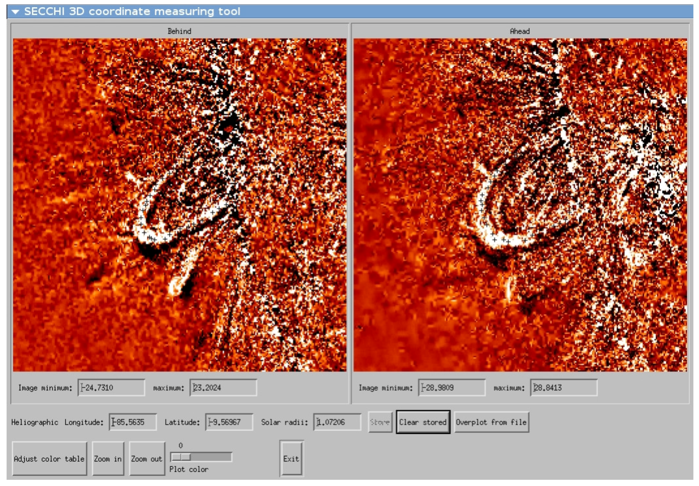
25]. The former includes a widget application (see 
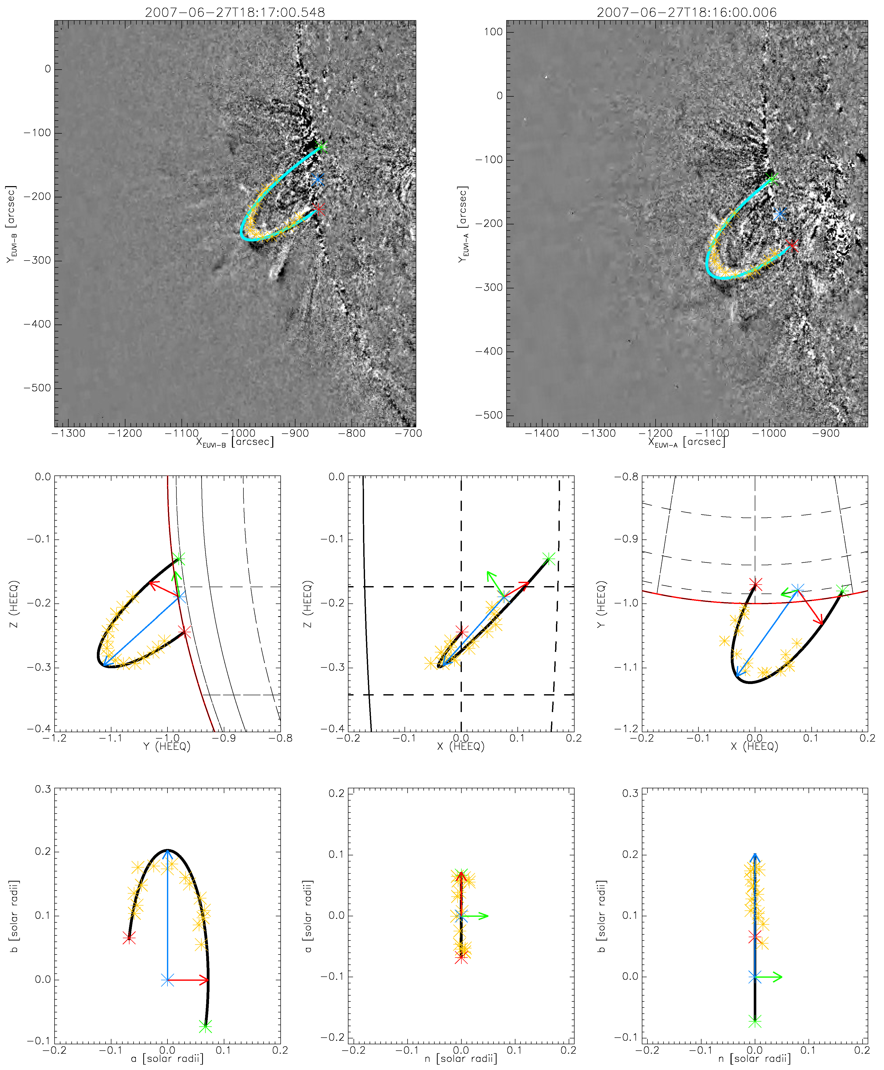
Figure 1 for a typical graphical output) that enables the user to select with the cursor a solar feature of interest appearing in both perspectives from one of the STEREO spacecraft (but it is also possible to combine SDO and the one of STEREO spacecraft). By selecting a point in one image, the program displays a line in the other image representing the LOS from the first image (or the epipolar line). The user then selects the point along this line with the same feature. The 3D coordinates are then calculated as (Earth-based) Stonyhurst heliographic longitude and latitude, along with the radial distance in solar radii. The coordinates can be easily converted into the Heliocentric Earth Equatorial (HEEQ) coordinates for a Cartesian representation of the data (for a complete review of the coordinate systems, please refer to [26]).
Figure 1. Graphical output of the procedure scc_measure: the windows give the field of view (FOV) from STEREO-A ( right) and STEREO-B ( left) spacecraft for a coronal loop on 27 June 2007, studied by Aschwanden [5], Verwichte et al. [14].
Entropy 15 04520 g001
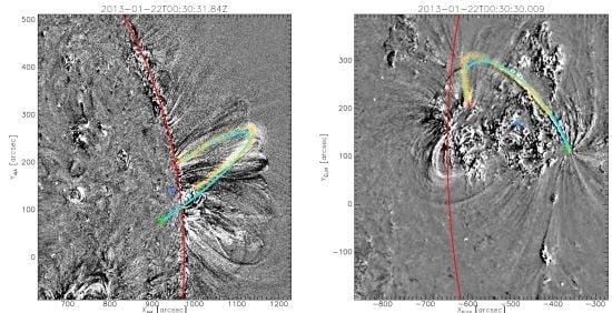
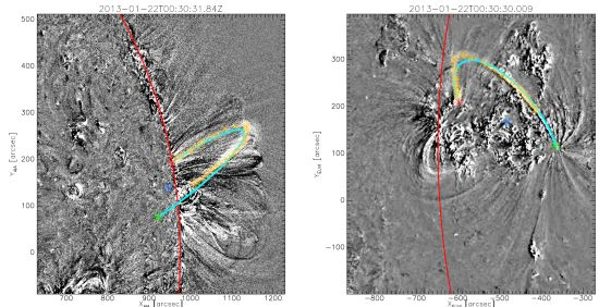
As we have seen, fitting a loop with a 1D curvilinear feature (circular or elliptical) depends on six parameters, namely: the heliographic longitude and latitude of the midpoint of the loop baseline on the solar surface, the baseline length between the two footpoints, the height of the loop, the inclination and the azimuth angle (see Section 3.4.4 of [27]).
A representation of the loop and its main parameters are shown in Figure 2. Recently, Gary et al. [28] proposed a fitting approach of loops by cubic Bézier curves, in order to distinguish between competing models for the magnetic field topology.
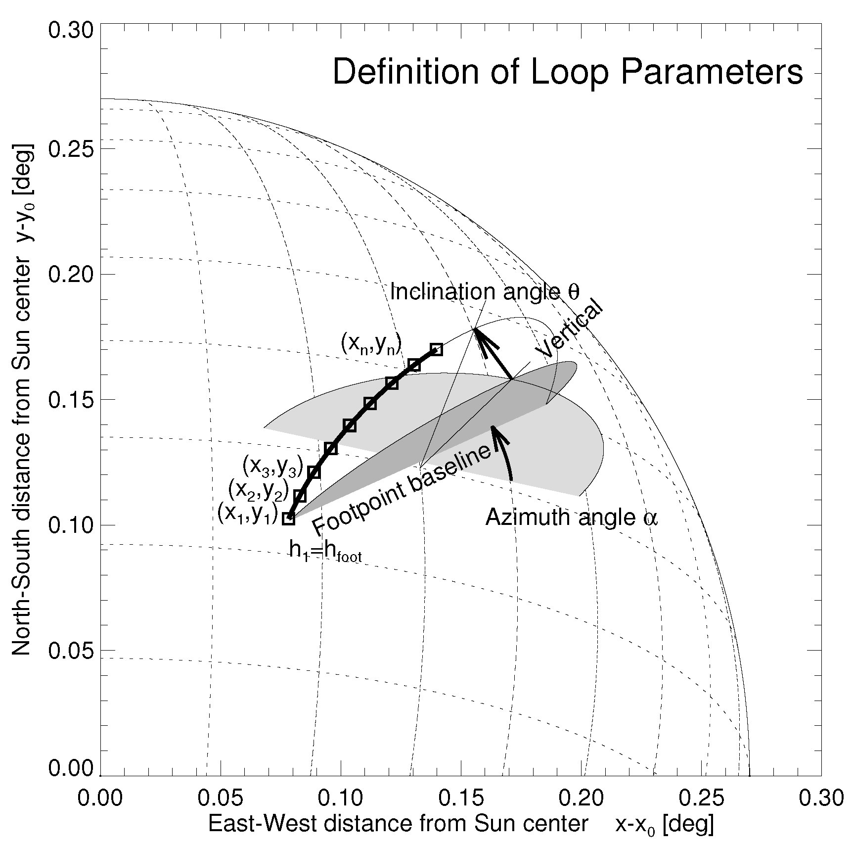
Figure 2. Schematic representation of a coronal loop relative to the solar surface, with the baseline connecting the footpoints, the inclination angle relative to the normal surface and the azimuth angle relative to the east-west direction. Courtesy of Markus Aschwanden.
Entropy 15 04520 g002
In this paper, we propose a new method allowing us to get the 3D shape of a loop by stereoscopic measurements, using principal component (PC) analysis. It reduces the number of parameters, dependencies and correlations between variables, by calculating a new basis of vectors, which defines the reference system relative to the loop. In the next section, we give an overview of PC analysis in the frame of 3D loop reconstruction. In Section 4, we present some examples, discussing analysis and comparing results with previous methods, and conclusions are given in the last section.

2. Three-Dimensional Reconstruction by Principal Component Analysis

Given a set of variables, which can be interrelated, PC analysis allows us to transform this set into a new one of “uncorrelated” or independent variables, known as principal components, but preserving the variation of the data distribution. Principal component analysis, also know as minimum variance analysis, has been applied in several research fields, e.g., in the determination of magnetic field geometry by in situ multi-spacecraft measurements [29]. Algebraically, PCs are particular linear combinations of the set of original variables, and geometrically, this is equivalent to the rotation of the original coordinate system into a new one, where the new axes represent the maximum variability of the dataset. Avoiding a rigorous mathematical treatment, which can be found in textbooks, such as Jolliffe [30], Johnson and Wichern [31], we give here a specific step-by-step description of how to fit coronal loops by PC analysis.
Given a set of N 3D data points x i = ( x i , y i , z i ) (we use, for simplicity, the HEEQ system) that sample the loop shape and is represented by an N × 3 matrix X, we can build the sample covariance matrix, S , defined as:
S = X T X = σ x , x 2 σ x , y 2 σ x , z 2 σ x , y 2 σ y , y 2 σ y , z 2 σ x , z 2 σ y , z 2 σ z , z 2
where σ q , q 2 = i = 1 N ( q i q ¯ i ) ( q i q ¯ i ) ), with q = x , y , z and q ¯ the mean, identified as the centre C = ( x ¯ , y ¯ , z ¯ ) of the loop. Now, we would like to put this in a new reference frame, whose axes maximise the variances, minimise the covariances of the points and have means equal to zero. This is equivalent to finding the eigenvalues and eigenvectors that diagonalise the matrix, S, in a matrix, Λ. Let us obtain the eigenvalues and sort them in the ascending order, as:
λ n λ a λ b
The corresponding eigenvectors will be e n , e a , e b , whose components are relative to the original frame. Thus, the matrix:
E = e n , x e n , y e n , z e a , x e a , y e a , z e b , x e b , y e b , z
defines the basis change X = E X l + C , and diagonalises S as Λ = E T S E (since E is the basis change matrix, E T = E 1 ); x l , i with i = 1 , . . . , N , are the coordinates of the data points in the new reference frame (they are also called “scores” in PC analysis); the eigenvector, e n , locates the normal to the loop plane, e a is directed like the minor axis of the ellipse and e b , like the major one. The axes values are related to the variance as (for statistical reasons, when N is small, it can be replaced by N 1 ):
a = 2 λ a N b = 2 λ b N
Indeed, since we have defined the covariance matrix, S , without dividing its elements by N, this should be done for the eigenvalues (the eigenvectors remain the same despite the normalisation of S ). A further justification for the presence of the factor, 2 , is given in Appendix A.1. The “fitted” loop can be traced starting from the parametric equations of an ellipse:
x e = a cos ( t ) y e = b sin ( t )
with t = [ 0 , 2 π ] , then, transformed in HEEQ coordinates, x e , y e , z e , by the basis change with the matrix E . Those points, whose squared distance satisfies the condition r 2 = x e 2 + y e 2 + z e 2 1 . 0 R , defines the loop curve.
We can look at how much of the total variance of the data points is counted by each single eigenvalue. Let Λ be the total variance defined as Λ = λ n + λ a + λ b . Then, the ratio λ i ^ = λ i / Λ (with i = n , a , b ) gives an indication of how much of the “energy” is carried out by λ i . According to Table 1, most of the variance is stored in along the e a , b directions, suggesting that the points are mostly distributed in a 2D plane. This is equivalent to saying that we have reduced the dimensionality of the dataset, by projecting it into a subspace, that is the 2D plane of the loop.
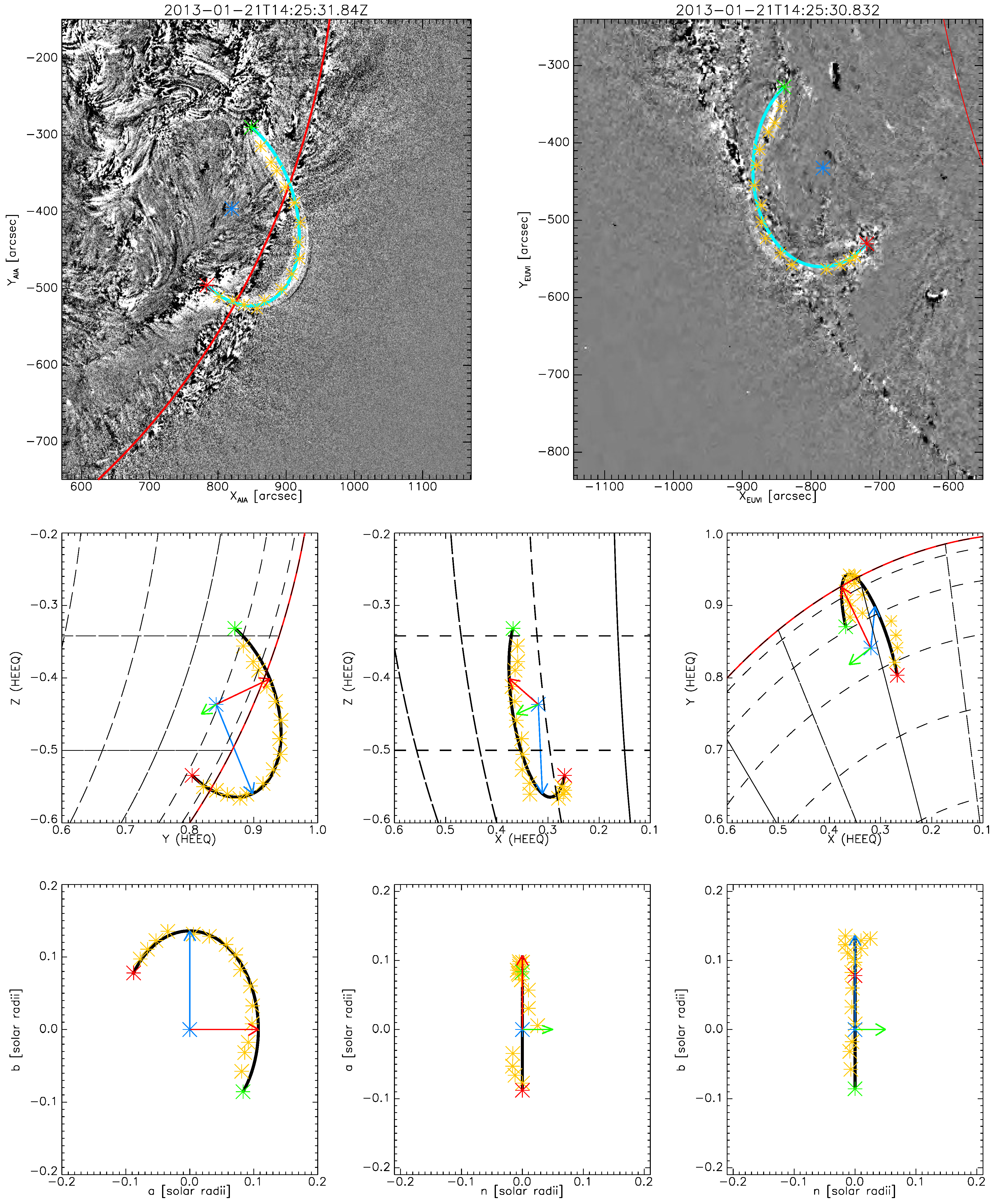
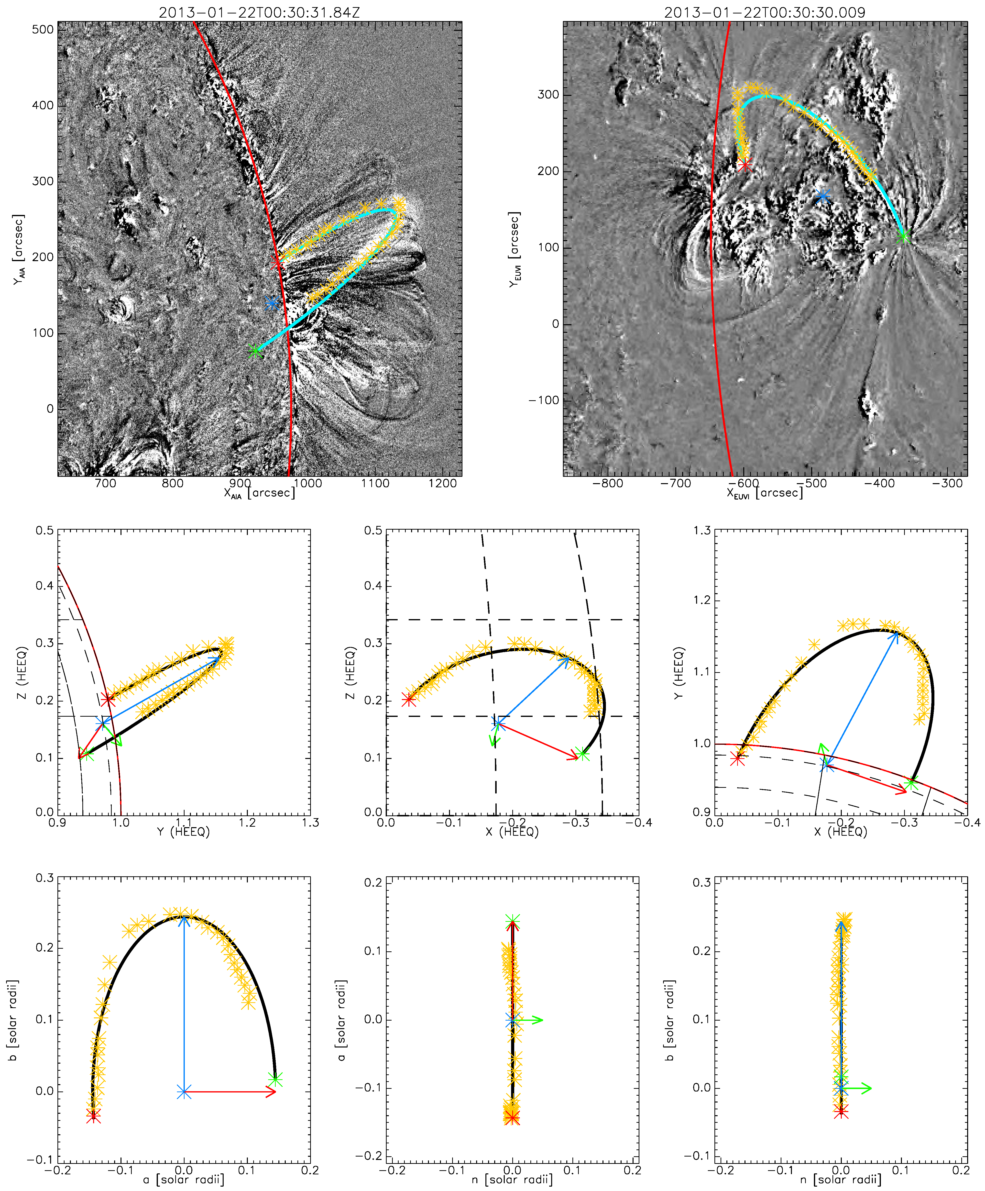
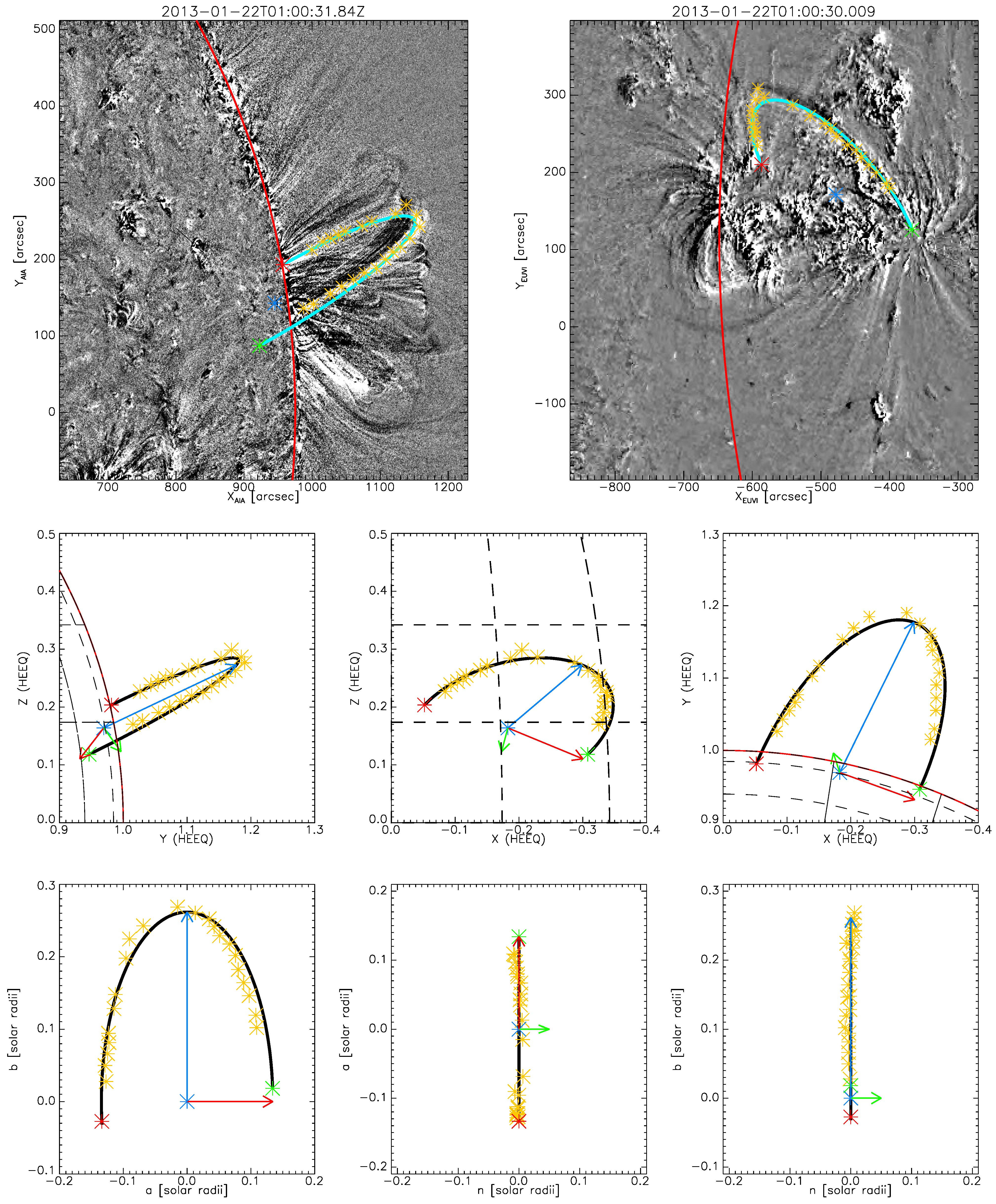
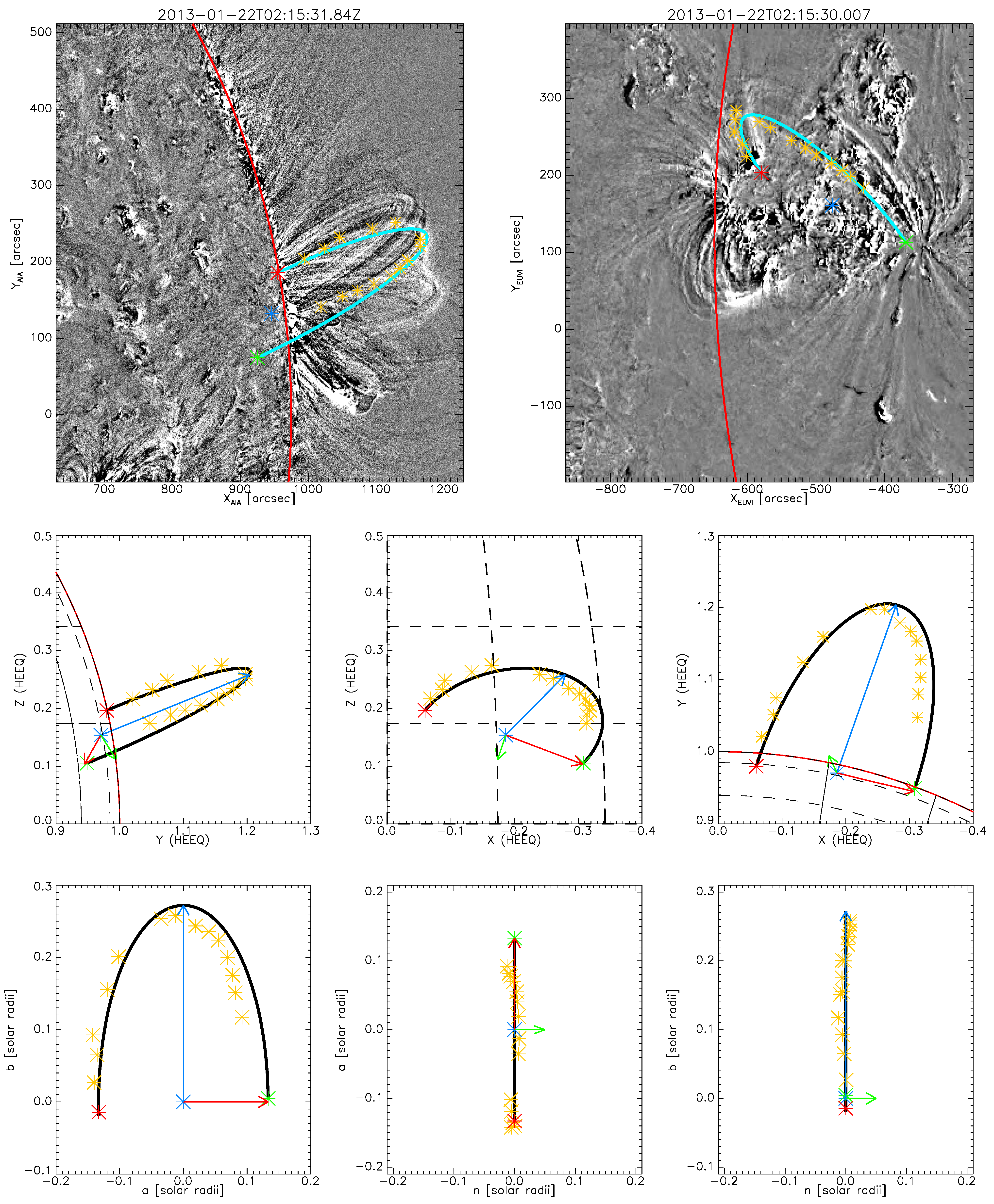
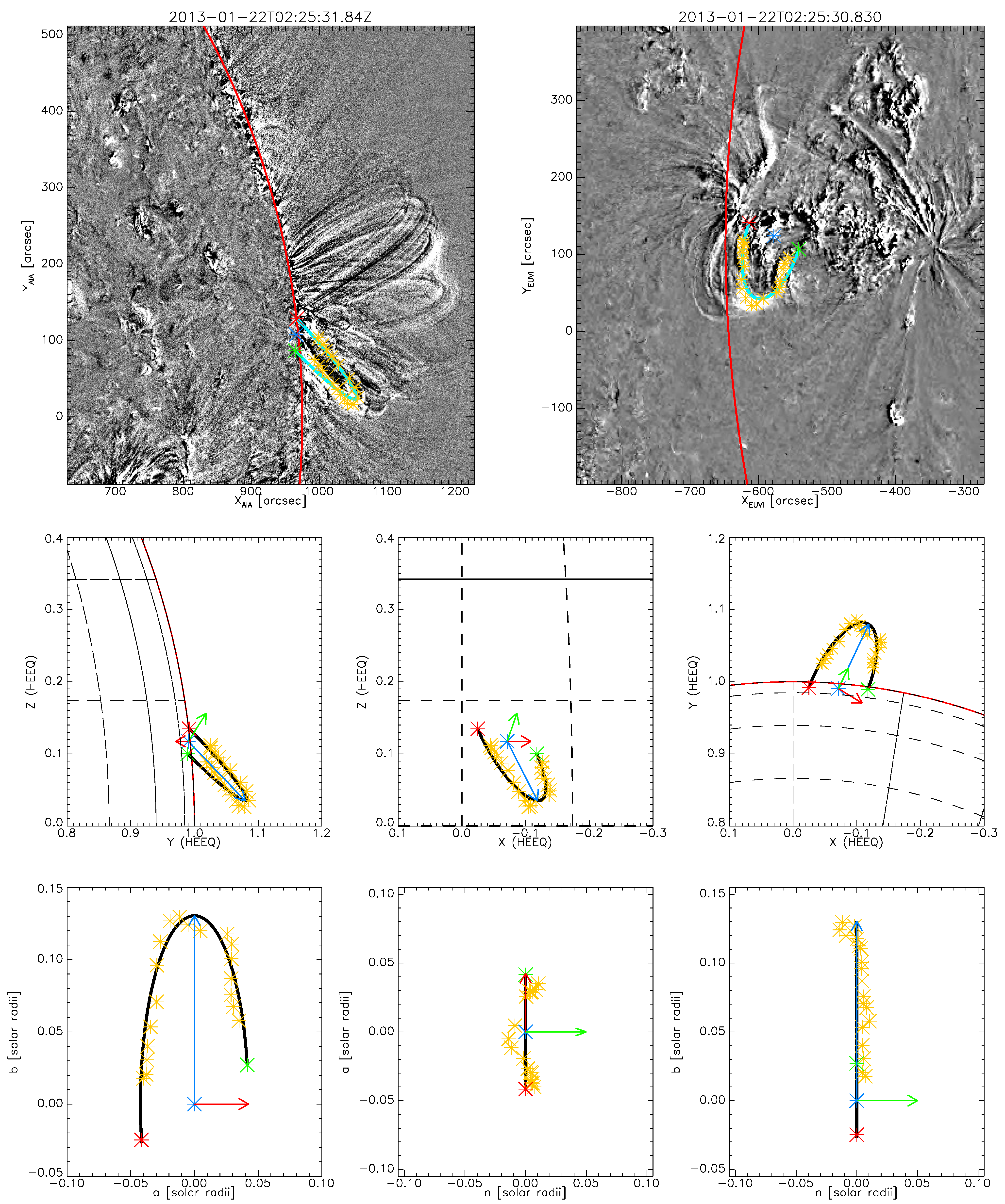
Table 1. The table shows the main quantities used and inferred from principal component (PC) analysis: the first rows are related to the inputs and show the number of 3D points, N, and the heliographic coordinates of the supposed loop centre; then, we tabulated the total variance, Λ, and the percentage relative to each eigenvalue, λ. The last rows show the estimates of each analysed loop: the minor (a) and major radii (b) with their corresponding standard deviations, the standard deviation, σ n , of the points from the loop plane, the inclination and azimuth angles, the eccentricity and, finally, the loop length.
Event2007-06-272013-01-212013-01-222013-01-222013-01-222013-01-22
(Figure)(3)(4)(5)(6)(7)(8)
N151530221419
ϕ C [deg]−87.7669.23100.35100.67100.8594.11
θ C [deg]−11.4125.889.259.438.846.74
Λ0.320.211.170.910.600.17
λ n ^ [%]0.240.800.040.050.090.50
λ a ^ [%]11.1738.0426.0320.8619.299.51
λ b ^ [%]88.5961.1673.9379.0980.6189.99
a [R ]0.072  0.1070.1450.1340.1330.042
σ a [R ]±0.004±0.008±0.006±0.006±0.010±0.003
b [R ]0.2020.1360.2440.2620.2720.130
σ b [R ]±0.014±0.004±0.011±0.010±0.019±0.007
σ n [R ]±0.008±0.011±0.004±0.004±0.006±0.007
θ [deg]2.850.0225.0620.6616.71−41.49
α [deg]37.21−72.62−17.34−17.17−19.63−15.20
eccentricity0.930.610.800.860.870.95
L [Mm]325.22276.62448.30457.96468.77203.64
We can obtain the inclination and azimuth angles from the orientation of the loop plane in space. The inclination angle is defined as the angle between the normal to the solar surface and the loop plane. By considering the vector, e n , normal to the loop plane, we can find the inclination angle as:
θ = π 2 cos 1 ( e r · e n )
where e r is the normal, directed in the radial directions. The azimuthal angle is defined as the angle formed by the intersection of the loop baseline with the east-west solar direction, represented by the longitudinal vector, e ϕ . Therefore, the azimuthal angle can be found as:
α = π 2 cos 1 ( e ϕ · e n )
The errors of the fitting can be estimated from the “scores” and their distance, d, from the fitted curve; it is possible to give an estimate of the standard deviation of the a and b direction from the sum of the squared distance (see A.2, for more details). Another possible way is to perform PC analysis for M samples of the 3D points, or to construct synthetic samples by randomly varying the 3D original measurements within their errors (private communication: Antonio Vecchio): the best values of the radii, inclinations and azimuth angles, as well as their standard deviations, will be inferred from their distributions.

3. Analysis and Discussion

In this section, we demonstrate some applications of PC analysis to specific coronal loops, with some comparisons with previous analysis.

3.1. The Event on 27 June 2007

The coronal loop in Figure 3 appeared on the east solar limb and was subject to kink oscillations, triggered by a flare. An analysis of the loop geometry is given in Verwichte et al. [14], using a forward modelling technique based upon the assumption of the circular shape, and in Aschwanden [5], with a fitting approach of the 3D stereoscopic points. The loop centre is not clearly identified, because of its proximity to the solar limb. The knowledge of the possible footpoints in Verwichte et al. [14], was inferred by looking at the same active region three days later, when it passed the east solar limb. Here, we deduce it directly from the stereoscopic measurements by calculating the centre of “mass” of the distribution of points and projecting the highest point (that can be regarded as the “apex” of the loop) to the solar surface, crossing the centre. Following this idea, we extrapolate a heliographic longitude of about ϕ C = 87 . 76 degand latitude θ C = 11 . 41 deg for the candidate loop centre. The results of the PC analysis are given in the first column of Table 1. We got an inclination of θ = 2 . 85 deg and an azimuth angle α = 37 . 21 deg . The relative errors for the minor and major radii are σ a / a = 5 . 6 % and σ b / b = 6 . 1 % , respectively. The loop length is about 325 Mm, and it is close to the value estimated by Aschwanden [5], Verwichte et al. [14]. Moreover, it exhibits a strong eccentricity (∼ 0 . 9 ), indicating an elliptical geometry rather than a circular one.
We overplotted the data points and the reconstructed loop over the AR seen three days later, on 30 June 2007. The loop seems to agree with the underlying topology of the AR, especially for the position of the footpoint labelled by green in Figure 4.

3.2. The Event on 21 January 2013

Here, we show a loop appearing in the quiet region on 21 January 2013, close to the western solar limb. The loop is seen well with SDO/AIA at 171, 193 Å, and visible in STEREO/EUVI-A, as well, but with a spatial resolution 2.5-times lower. We were able to take 3D points with scc_measure: we worked on filtered images (we subtracted the frames with those 5 min previous) in order to highlight the loop shape (Figure 5-top). Since the footpoints are well identified, we determined the centre as the midpoint between footpoints. We took 10 independent measurements and considered their mean as the best value for the centre. The outcomes of PC analysis are listed in Table 1.
Figure 3. A coronal loop on the east solar limb during a flare event on 27 June 2007. The event was studied by Aschwanden [5], Verwichte et al. [14]. The top figures show the FOVs from STEREO-A (right) and STEREO-B (left). The yellow symbols are the 3D data points measured with the routine scc_measure. The light-blue line is the fitted curved loop; at the base, the centre is in blue, and the footpoints inferred from the reconstruction are in red and green colours. The middle plots show the reconstructed loop against the yellow data points, for the different orientations of the Heliocentric Earth Equatorial (HEEQ) coordinates system. The coloured vectors represent the new set of three axes: in red and blue, the minor and major axis; in green, the normal to the loop plane. Indeed, the bottom figures show the loop in this new reference frame for different orientations. A similar description is applied for the Figures of the other analysed events.
Entropy 15 04520 g003
Figure 4. Image from STEREO-B at 171 Å of the active region, which was the site of the analysed coronal loop, on 30 June 2007. The 3D points and the “fitted” loop are overplotted in order to visually prove the consistency of our results. Note that there is a good agreement with the position of the top-right footpoint with the open loops of the active regions. The red meridian marks the position of the solar limb on 27 June 2007.
Entropy 15 04520 g004

3.3. The Event on 22 January 2013

Here, we present the 3D reconstruction of coronal loops belonging to the active region AR NOAA (National Oceanic and Atmospheric Administration) 11654, studied by Anfinogentov et al. [32]. The active region exhibits a large number of coronal loops. From SDO/AIA, the active region is partly off-limb, and loop footpoints are not visible. The same active region is seen well from STEREO-A: the footpoints are easily identified, and the loops seem to span for a wide angle across the surface normal. Therefore, intuitively, one could assume that the only parameter that is changing is the inclination angle, θ, while the other properties, like the loop lengths and the azimuth angles, α, should remain almost constant. We use running difference images, in order to identify the loop in both FOVs when we note a simultaneous intensity variation. Figure 6, Figure 7 and Figure 8 show the reconstruction for some of these loops, which were located with good certainty. The parameters are listed in Table 1; for all three loops, note the consistency in the parameters, like the minor and major radii, the eccentricity, the azimuth angle and the loop length. Furthermore, one can see the discrepancy in the estimation of the inclination, suggesting that the analysed loops become gradually more perpendicular to the solar surface. The loop in Figure 9 is different, showing different geometrical values and a stronger inclination.
Figure 5. The coronal loop event observed with SDO/AIA (left) and STEREO-A (right) in a quiet region on 21 January 2013, in the Southern hemisphere.
Entropy 15 04520 g005
Figure 6. Analysis of the loop (a) on 22 January 2013.
Entropy 15 04520 g006
Figure 7. Analysis of the loop (b) on the 22 January 2013.
Entropy 15 04520 g007
Figure 8. Analysis of the loop (c) on the 22 January 2013.
Entropy 15 04520 g008
Figure 9. Analysis of the loop (d) on the 22 January 2013.
Entropy 15 04520 g009

4. Conclusions

In this paper, we propose a new method for the determination of the 3D shape of coronal loops from stereoscopic measurements. The necessity to understand the loop shape is important in order to better estimate, for example, the loop length, which is a crucial parameter in inferring the magnetic field by coronal seismology (or, generally, to compare the geometry of loops, which are assumed to trace magnetic field lines in the low-β coronal plasma, with potential field models of the coronal magnetic field [28]). Furthermore, the loop shape determines the variation of the column depth along the loop in different phases of kink oscillations and, hence, the distribution and dynamics of the LOS-integrated intensity of the loop. The previous approach to 3D reconstruction is based on fitting stereoscopic 3D tie-points, taken along the loops. A good fitting requires a large number of points, but taking them could be a laborious task, because of high observational and instrumental noise and the effect of the LOS integration. Usually, by procedures, e.g., scc_measure, the number of tie-points selected is about 10–20. The method used in Aschwanden et al. [21] and his subsequent papers is to interpolate the 3D points with a spline, in order to retrieve the loop shape. On the other hand, this operation could add further degrees of freedom (e.g., non-planarity), and the corresponding reconstructed loop could deviate from a regular shape, like a circle or ellipse (e.g., see Figure 9 of Aschwanden et al. [21], and Figure 7 of Aschwanden [5]), also because of the natural spread of the measurements around the true value. Moreover, fitting the 3D points with a 1D curvilinear feature requires the determination of the six free parameters: the inclination and azimuth angles, the length of the baseline, the loop centre position and the loop height. Conversely, all this information is implicitly stored in the distribution of a sample of 3D measurements, and it can be retrieved easily by the technique of principal components analysis. Determination of these parameters can be made by a simple step-by-step process. The technique we developed can be summarised in the followings steps:
  • measurement of a sample of 3D tie-points that outline the loop shape from two different LOSs;
  • calculation of the sample covariance matrix, S , of the 3D points;
  • determination of the three pairs of eigenvalue/eigenvectors, λ i / e i , which identify the new reference frame relative to the loop, sorted in ascending order;
  • the smallest eigenvalues and the corresponding eigenvector is associated with the normal to the loop plane;
  • the largest eigenvalue/eigenvector locates the major axis and the remaining, the minor axis, according to Equation (4);
  • determination of the inclination and azimuth angles according to Equations (6) and (7);
  • loop tracing with the parametric Equation (5) and transformation in the original coordinates system, HEEQ.
The determination of the set of three vectors, e n , e a , e b 
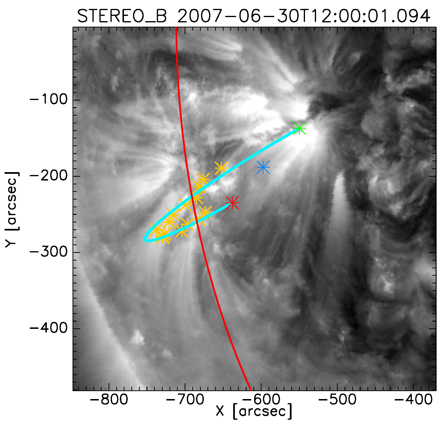
, which constitutes the new basis for the reference frame relative to the loop, depends uniquely on the choice of the loop centre (or, also, called the midpoint), which plays the role of the decisive parameter of the problem. Moreover, according to the example of the loop on 27 June 2007 (Figure 3), we have shown that the information about the midpoint can be deduced or guessed directly from the 3D measurements, overcoming the issue of the lack of information about the loop baseline, when it is too close to the solar limb. The advantage of this method is that it works for a reasonably small number of data points (10–20), without requiring any intermediate step, like interpolation. The only assumption made in our analysis is the planarity of the loop, but possible speculations on it can be made by studying the distribution of the data points around the loop plane and searching for some possible patterns, like arcs or s-shapes, which could outline, respectively, the fundamental and second harmonic in kink oscillations. On the other hand, the relative deviation of the measurements from the best-fitted loop plane is less the 1%, probably too small in order to appreciate any non-planarity. Moreover, a further step forward for reasonable modelling of the magnetic field would be to fit the loop shape by a dipole or stretched dipole line, as suggested in Hu et al. [33]. These issues, as well as refinements of the technique by PC analysis could be the object of future work.

Acknowledgments

The authors thank the STEREO/SECCHI and SDO/AIA scientific teams for the data provided. The authors would like to thank also the UK-Science and Technology Facilities Council (STFC) for the Centre for Fusion, Space and Astrophysics (CFSA) Rolling Grant. G.N. thanks Antonio Vecchio for useful discussion. The work of V.M.N. is also supported by the European Research Council under the SeismoSun Research Project, No. 321141, the Russian Ministry of Education and Science, project No. 8524, the Russian Foundation of Basic Research under grant 13-02-00044 and the Kyung Hee University International Scholarship (V.M.N.).

Conflicts of Interest

The authors declare no conflict of interest.

A. Appendix

A.1. Coronal Loops As a Bivariate Normal Distribution

The distribution of 3D points that identifies coronal loops can be regarded as a case of multivariate normal distribution (see Chapter 4 and 8 of [31]). The univariate normal distribution, with the mean, μ , and variance σ 2 , has the probability density function:
f ( x ) = 1 2 π σ 2 exp [ ( x μ ) / σ ] 2 / 2
where the term:
1 2 x μ σ 2 = 1 2 ( x μ ) ( σ ) 2 ( x μ )
measures the squared distance from x to μ in the standard deviation units. For N observations of a vector, x , this can be represented by:
1 2 ( x μ ) Σ 1 ( x μ )
with μ being the expected value and Σ being the variance-covariance matrix of the x observations (the apex indicates the complex conjugate of ( x μ ) , and similarly in the next equations, as well). The above quantity for a multivariate distributions represents the contour of constant density probability at specific values k 2 , or the surface of an ellipsoid centred in μ. In our case, given the x i observations, the centre, C, and the sample covariance matrix, S , we have:
1 2 ( x C ) S 1 ( x C ) = k 2 = 1 2 x l Λ 1 x l
because of the principal components reduction. Therefore, if we expand the right side of Equation (11), we get the equation of a 3D ellipsoid:
x l , a 2 2 λ a 2 + x l , b 2 2 λ b 2 + x l , n 2 2 λ n 2 = k 2
Since the eigenvalues, λ n , do not significantly contribute to the total variance, they can be eliminated, and we get the equation of an ellipse in the canonical form, with k = 1 , a = 2 λ a , b = 2 λ b :
x l , a 2 a 2 + x l , b 2 b 2 = 1

A.2. Error Estimations

The errors in the fitting can be estimated from the “scores” or the distance from the fitted curve. Let x l = ( x l , a , x l , b , x l , n ) be the data point in the loop reference frame and x e = ( x e , a , x e , b , x e , n ) , a point of the fitted curve (that should be determined). The squared distance, d 2 , will be:
d 2 = d a 2 + d b 2 + d n 2 = ( x l , a x e , a ) 2 + ( x l , b x e , b ) 2 + ( x l , n x e , n ) 2
Let us normalise the distance along the axes to the radii, a and b:
d a 2 = a ( x ^ l , a x ^ e , a ) 2 d b 2 = b ( x ^ l , b x ^ e , b ) 2
Now, we have reduced the loop to a circumference of radius 1. The coordinates, x ^ e , a and x ^ e , b , will be, respectively, equal to the cosine and sine of the angle spotted by the point, ( x ^ l , a , x ^ l , b ) , so that we rewrite as:
x ^ e , a = cos γ = x ^ l , a x ^ l , a 2 + x ^ l , b 2
x ^ e , b = sin γ = x ^ l , b x ^ l , a 2 + x ^ l , b 2
and hence:
d a 2 = a x ^ l , a ( 1 1 x ^ l , a 2 + x ^ l , b 2 ) 2 d b 2 = b x ^ l , b ( 1 1 x ^ l , a 2 + x ^ l , b 2 ) 2
The standard deviation along a, b and n can be estimated as:
σ j = i N d i , j 2 N 1 with j = ( a , b , n )

A.3. Error Estimate on the Loop Length

The loop length can be estimated numerically given the radii, a and b, and N p grid points along the loop as:
L = i = 2 N p l i = i = 2 N p x e , a ( i ) x e , a ( i 1 ) 2 + x e , b ( i ) x e , b ( i 1 ) 2
In the polar representation, we have:
L = i = 2 N p a 2 ( cos γ i cos γ i 1 ) 2 + b 2 ( sin γ i sin γ i 1 ) 2
i = 2 N p a 2 ( cos γ i cos γ i 1 ) 2 + b 2 ( sin γ i sin γ i 1 ) 2
= a i = 2 N p ( cos γ i cos γ i 1 ) + b i = 2 N p ( sin γ i sin γ i 1 )
The uncertainty of the length can be expressed as (note that, in general, the inequality ln ( x + y ) ln ( x ) + ln ( y ) is true when x y / ( y 1 ) ):
Δ L L d ln L d ln a i = 2 N p ( cos γ i cos γ i 1 ) + d ln b i = 2 N p ( sin γ i sin γ i 1 )
d ln a + d ln b Δ a a + Δ b b
For very good fittings, we obtained the uncertainties, σ a / a and σ b / b , of the order of 3–5%, so that the loop length error should be less than 8 %.

References

  1. Cooper, F.C.; Nakariakov, V.M.; Tsiklauri, D. Line-of-sight effects on observability of kink and sausage modes in coronal structures with imaging telescopes. Astron. Astrophys. 2003, 397, 765–770. [Google Scholar] [CrossRef] [Green Version]
  2. Cooper, F.C.; Nakariakov, V.M.; Williams, D.R. Short period fast waves in solar coronal loops. Astron. Astrophys. 2003, 409, 325–330. [Google Scholar] [CrossRef]
  3. Kaiser, M.L.; Kucera, T.A.; Davila, J.M.; St. Cyr, O.C.; Guhathakurta, M.; Christian, E. The STEREO mission: An introduction. Space Sci. Rev. 2008, 136, 5–16. [Google Scholar] [CrossRef]
  4. Bosman, E.; Bothmer, V.; Nisticò, G.; Vourlidas, A.; Howard, R.A.; Davies, J.A. Three-dimensional properties of coronal mass ejections from STEREO/SECCHI observations. Solar Phys. 2012, 281, 167–185. [Google Scholar] [CrossRef]
  5. Aschwanden, M.J. The 3D geometry, motion, and hydrodynamic aspects of oscillating coronal loops. Space Sci. Rev. 2009, 149, 31–64. [Google Scholar] [CrossRef]
  6. Aschwanden, M.J.; Fletcher, L.; Schrijver, C.J.; Alexander, D. Coronal loop oscillations observed with the transition region and coronal explorer. Astrophys. J. 1999, 520, 880–894. [Google Scholar] [CrossRef]
  7. Nakariakov, V.M.; Ofman, L.; Deluca, E.E.; Roberts, B.; Davila, J.M. TRACE observation of damped coronal loop oscillations: Implications for coronal heating. Science 1999, 285, 862–864. [Google Scholar] [CrossRef] [PubMed]
  8. Tomczyk, S.; McIntosh, S.W.; Keil, S.L.; Judge, P.G.; Schad, T.; Seeley, D.H.; Edmondson, J. Alfvén waves in the solar corona. Science 2007, 317, 1192–1196. [Google Scholar] [CrossRef] [PubMed]
  9. Wang, T.; Ofman, L.; Davila, J.M.; Su, Y. Growing transverse oscillations of a multistranded loop observed by SDO/AIA. Astrophys. J. Lett. 2012, 751. [Google Scholar] [CrossRef]
  10. White, R.S.; Verwichte, E. Transverse coronal loop oscillations seen in unprecedented detail by AIA/SDO. Astron. Astrophys. 2012, 537, A49. [Google Scholar] [CrossRef]
  11. Nisticò, G.; Nakariakov, V.M.; Verwichte, E. Decaying and decayless transverse oscillations of a coronal loop. Astron. Astrophys. 2013, 552, A57. [Google Scholar] [CrossRef]
  12. Nakariakov, V.M.; Ofman, L. Determination of the coronal magnetic field by coronal loop oscillations. Astron. Astrophys. 2001, 372, L53–L56. [Google Scholar] [CrossRef]
  13. Van Doorsselaere, T.; Brady, C.S.; Verwichte, E.; Nakariakov, V.M. Seismological demonstration of perpendicular density structuring in the solar corona. Astron. Astrophys. 2008, 491, L9–L12. [Google Scholar] [CrossRef]
  14. Verwichte, E.; Aschwanden, M.J.; van Doorsselaere, T.; Foullon, C.; Nakariakov, V.M. Seismology of a large solar coronal loop from EUVI/STEREO observations of its transverse oscillation. Astrophys. J. 2009, 698, 397–404. [Google Scholar] [CrossRef]
  15. Verwichte, E.; Foullon, C.; van Doorsselaere, T. Spatial seismology of a large coronal loop arcade from TRACE and EIT observations of its transverse oscillations. Astrophys. J. 2010, 717, 458–467. [Google Scholar] [CrossRef]
  16. Aschwanden, M.J.; Newmark, J.S.; Delaboudinière, J.P.; Neupert, W.M.; Klimchuk, J.A.; Gary, G.A.; Portier-Fozzani, F.; Zucker, A. Three-dimensional stereoscopic analysis of solar active region loops. I. SOHO/EIT observations at temperatures of (1.0–1.5) × 106 K. Astrophys. J. 1999, 515, 842–867. [Google Scholar] [CrossRef]
  17. White, R.S.; Verwichte, E.; Foullon, C. First observation of a transverse vertical oscillation during the formation of a hot post-flare loop. Astron. Astrophys. 2012, 545, A129. [Google Scholar] [CrossRef]
  18. White, R.S.; Verwichte, E.; Foullon, C. Anti-phase signature of flare generated transverse loop oscillations. Astrophys. J. 2013. [Google Scholar] [CrossRef]
  19. Verwichte, E.; Van Doorsselaere, T.; Foullon, C.; White, R.S. Coronal Alfvén speed determination: Consistency between seismology using AIA/SDO transverse loop oscillations and magnetic extrapolation. Astrophys. J. 2013, 767. [Google Scholar] [CrossRef]
  20. Inhester, B. Stereoscopy basics for the STEREO mission. 2006; arXiv:astro-ph/0612649. [Google Scholar]
  21. Aschwanden, M.J.; Wülser, J.P.; Nitta, N.V.; Lemen, J.R. First three-dimensional reconstructions of coronal loops with the STEREO A and B spacecraft. I. Geometry. Astrophys. J. 2008, 679, 827–842. [Google Scholar] [CrossRef]
  22. Aschwanden, M.J. Loop 3D-geometry modeling-software tutorial. Available online: http://www.lmsal.com/aschwand/software/loopgeo/loopgeo_tutorial1.html (accessed on 24 August 2013).
  23. SolarSoft. Available online: http://www.lmsal.com/solarsoft/ (accessed on 24 August 2013).
  24. Scc measure.pro. Available online: http://hesperia.gsfc.nasa.gov/ssw/stereo/secchi/idl/display/scc_measure.pro (accessed on 24 August 2013).
  25. Sunloop.pr. Available online: hesperia.gsfc.nasa.gov/ssw/stereo/secchi/idl/display/sunloop/sunloop.pro (accessed on 24 August 2013).
  26. Thompson, W.T. Coordinate systems for solar image data. Astron. Astrophys. 2006, 449, 791–803. [Google Scholar] [CrossRef]
  27. Aschwanden, M.J. Physics of the Solar Corona. An Introduction; Praxis Publishing Ltd: Omaha, NE, USA, 2004. [Google Scholar]
  28. Gary, G.A.; Hu, Q.; Lee, J.K. A rapid, manual method to map coronal-loop structures of an active region using cubic Bézier curves and its applications to misalignment angle analysis. Solar Phys. 2013. [Google Scholar] [CrossRef]
  29. Sonnerup, B.U.Ö.; Scheible, M. Minimum and Maximum Variance Analysis. In Analysis Methods for Multi-Spacecraft Data; ISSI Scientific Reports Series; Paschmann, G., Daly, P., Eds.; ISSI/ESA: Bern, Switzerland, 1998; Volume 1, pp. 185–220. [Google Scholar]
  30. Jolliffe, I.T. Principal Component Analysis; Springer: New York, NY, USA, 1986. [Google Scholar]
  31. Johnson, R.A.; Wichern, D.W. Applied Multivariate Statistical Analysis; Pearson Prentice Hall: Upper Saddle River, NJ, USA, 2007. [Google Scholar]
  32. Anfinogentov, S.; Nisticò, G.; Nakariakov, V.M. Decayless kink oscillations in coronal loops. Astron. Astrophys. 2013. [Google Scholar] [CrossRef]
  33. Hu, Q.; McKenzie, J.F.; Webb, G.M. Klein-Gordon equations for horizontal transverse oscillations in two-dimensional coronal loops. Astron. Astrophys. 2012, 541, A53. [Google Scholar] [CrossRef]

