1. Introduction
Electrostatic interactions play an important role in many nano- or meso-scale systems. Almost every surface immersed in water develops a significant surface charge, due to the acid-base reactions of surface groups, and most biomolecules also carry charges. Therefore, it is often indispensable to include these long-ranged interactions in computer simulations. However, the system sizes that can be handled in simulations are orders of magnitude smaller than in real experiments, which drastically enhances the influence of boundary effects. To avoid artifacts due to an artificially small simulation volume, one typically uses periodic boundary conditions (PBC), which in simulations have to be taken into account by special electrostatics algorithms. These are often based on the idea of the Ewald summation [
1,
2,
3,
4], namely splitting the potential into a smooth, long-ranged and a singular, short-ranged contribution. In modern computer simulations, one usually uses mesh-based variants of the Ewald summation [
5,
6,
7,
8], which have a favorable
computing time scaling with respect to the number of charged particles,
N.
When studying capacitors, membranes or thin films, one does not want PBC perpendicular to the surfaces of interest. For these systems, partially periodic boundary conditions with only two periodically replicated dimensions are desirable, while the third one has a finite extent
h (
geometry). For these geometries, the Ewald summation becomes ineffective [
9]. However, it has been shown that replicating the system artificially in the direction perpendicular to the surface results in reasonable accuracy when compared to the non-periodic system, provided a sufficient gap is left between the replicas, and a correction term for the summation order is included [
10]. The ELC (electrostatic layer correction) approach [
11,
12] can, in principal, compute electrostatic interactions with the charges in the unwanted periodic dimension exactly. Practically, it allows one to tune the gap size to a desired accuracy, so that the
geometry is computationally tractable with any Coulomb solver for 3D PBC. It has to be stated that an algorithmic approach for partially periodic systems has been presented in [
13,
14] using a Monte Carlo extension to the local update scheme sketched in
Section 5, but it is not implemented into the molecular dynamics implementation used for this article.
When studying large-scale problems, for example, the buckling of membranes, solutions containing charged polymers or colloids, DNA translocation or crystallization of charged colloids, an atomistic representation of the system under study is often unfeasible, even with periodic boundary conditions. This is related to the vast numbers of charges that would need to be treated, but also with the unfavorable scaling of the relaxation times of the system. One popular route to tackle such problems is to use implicit solvent models, which electrostatically represent the solvent as an effective dielectric medium of the representative dielectric constant at the investigated temperature. This works well if particles, for example, colloids or polymers, are in bulk solution, since, then, the dielectric medium is isotropic and, to a good approximation, homogeneous. However, if surfaces are involved, the dielectric constant of the solvent is usually drastically different from the material forming the surface. For example, water at room temperature has a dielectric constant of , while a typical membrane has a dielectric constant of .
In systems with spatial variations of the dielectric constant, the Poisson equation for electrostatics reads as:
with the permittivity
, the electrostatic potential, Φ, and the charge distribution,
ρ. Equation (
1) leads to complex boundary conditions at dielectric interfaces, which need to be taken into account by the underlying electrostatics method. Conducting media can, in principle, be treated as the
limit of the above equation and, thus, allow one to treat this case with very similar methods to those for dielectric contrast. Since these materials appear in important fields, such as energy storage and electrolyte capacitors, our described methods of treating dielectric contrast will also be useful there.
In the following, we will describe how to fulfill the dielectric boundary conditions for planar surfaces using the concept of image charges [
15,
16,
17]. These approaches can even be extended to the special case of two
connected conducting surfaces. As an alternative route, we present the ICC* (induced charge calculation) algorithm, which can handle arbitrarily-shaped surfaces [
18,
19]. Instead of computing image charge interactions, which is only feasible in some simple geometries, the method determines the induced charges at the surfaces self-consistently.
Both image charge and induced charge approaches can only handle boundaries between media of otherwise constant dielectric properties. In this article, we will also describe an extension of the Maxwell Equations Molecular Dynamics (MEMD) algorithm [
20,
21], which can also handle continuously varying dielectric constants. It solves a simplified version of the Maxwell electrodynamics equations on a discrete lattice.
The methods and results presented in this review were mostly published before in [
16,
17,
18,
19,
22]. Implementations of all methods, including the features discussed here, can be found in ESPResSo, the Extensible Simulation Package for Research on Soft matter [
22,
23]. A review article on the general topic of long-range interactions in soft matter can be found in [
24].
2. Planar Interfaces: Image Charges
We start by discussing the simplest case of dielectric interfaces, namely, two planar, parallel interfaces that enclose a set of charges. We assume a vertical orientation of the interfaces and refer to a left and a right (l/r) interface. The electric field between the two interfaces can be computed from these charges, plus additional image charges outside of the dielectric boundaries [
25]. The positions and magnitude of these images charges are chosen to satisfy the boundary conditions for the electric field. If only one interface, the left or the right interface, were present, image charges would appear reflected at the respective interface, with the charge scaled down by a factor of:
where
is the background permittivity in the main cell and
and
are the permittivities in the adjacent left and right media, respectively. Note that
and
can be positive, as well as negative, so that a charge can be attracted to the wall or repelled by it.
To construct the image charges in a situation with two interfaces, every image charge created by reflection on one interface also needs to be reflected again onto the other interface. This leads to an infinite set of images: A charge,
q, is reflected at the right (left) interface and yields an image of the magnitude of
(resp.
). The next reflection gives rise to another image charge,
(resp.
), in the opposite dielectric domain, and so on. The infinite array of image charges is depicted in
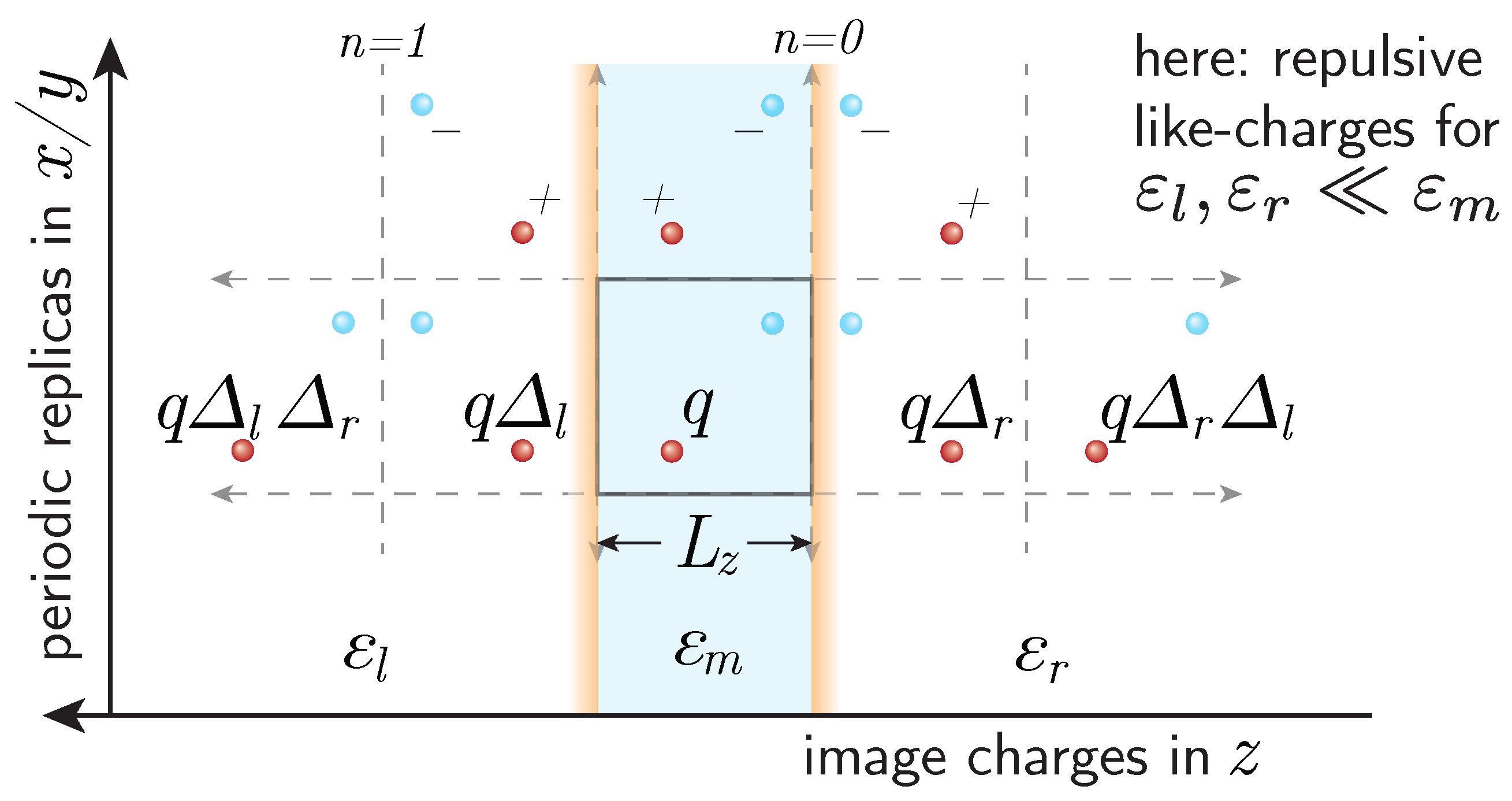
Figure 1: a charge,
q, at position
z will produce a series of mirror charges in the right dielectric domain (with
) with charges:
where
denotes the distance between the two interfaces and
. In the left dielectric domain (with
), the charges are:
Figure 1.
Schematic summation scheme for Image Charge MMM2D (ICMMM2D): in order to take into account dielectric boundaries, image charges are introduced outside the dielectric boundaries, to the left and right of the original box. The dielectric contrasts, and , are computed from the dielectric jump at the left and right boundaries, respectively. Depending on the dielectric contrasts, charges will either be repelled by the surface (as in this sketch) or attracted to it. Note that in usual computer simulations, the system is periodically replicated in the dimensions parallel to the interfaces, as indicated in the figure.
When computing the electrostatic interaction in a computer simulation with such parallel, infinite planar walls, it is often desired to employ periodic boundary conditions in the two directions parallel to the walls to minimize surface effects. The direct summation of periodic replicas is very costly, as the sum is only slowly convergent. Thus, special techniques to compute the electrostatic interactions are required. MMM2D is such an algorithm that computes the electrostatic interaction with two periodic dimensions [
26,
27] and is well suited for computing the interactions with the image charges. The key idea of the MMM2D algorithm is to use two different formulas for the interaction of two charges. One of the formulas, the near formula, is only used if the two particles are sufficiently close. In combination with image charges, it is only used for the closest of all images, and its discussion is beyond the scope of this article.
The second, far formula is accurate if a certain distance between the two charges is exceeded. We assume a simulation box of
that is periodically replicated in the
x and
y dimensions. Then, the Coulomb potential of a unit charge placed at the origin evaluated at position
with
, including periodic replicas in the
x and
y direction, can be written as:
where
. This formula follows from a Fourier transformation of the Poisson equation in the
x and
y direction and can be factorized into contributions. This makes it possible to compute the interactions between
N separated charges in
operations. Due to the unfavorable scaling of the near formula, MMM2D scales only like
overall. It, however, is still superior to Ewald-based methods [
9] in partially periodic boundary conditions.
Coming back to our original problem of taking into account the infinite array of image charges, we note that all these charges, with the exception of those directly adjacent, i.e., with index
, are far from the slab containing the real charges. Therefore, we can apply the fast far formula in order to compute the interaction with these charges. The infinite sums of image charges lead to geometric series of the form:
which is a geometric series that can be easily simplified to:
In other words, an existing implementation of MMM2D can be easily enhanced in order to include dielectric interfaces, simply by modifying the prefactors of the
-Fourier sum. For the detailed expressions, see [
16]. In the following, we denote such an MMM2D implementation for dielectric interfaces as ICMMM2D (Image Charge MMM2D).
Note that Equation (
5) contains an additional term,
, which represents the constant Fourier mode. The summation over the image charges of this term leads to expressions of the form:
since
is larger than any possible particle distance
z. Unlike Equation (
6), this is not a simple geometric series. However, when computing the total potential in a charge neutral system, terms that do not depend on the positions cancel out, in particular, the
terms. What remains from the four image charge sums are again geometric series that lead to a contribution of:
If the two planar walls have the same dielectric contrast, this contribution to the potential vanishes. Furthermore, if one is only interested in energy or forces, this contribution vanishes, due to charge neutrality.
An alternative method for planar dielectric interfaces is based on an extension of our ELC method. It also uses the technique to sum up the image charges with the ICMM2D far formula, and we termed it ELCIC (ELC with Image Charges), see [
17] for details of the method.
Note that it is also possible to consider systems that are not charge neutral. Formally, one assumes two equally charged plates at the positions of the dielectric interfaces that cancel the total charge [
28]. The field of a charged plate is, however, exactly what the
term represents, so that the above considerations for this term still hold. Therefore, one can safely ignore this contribution.
Figure 2.
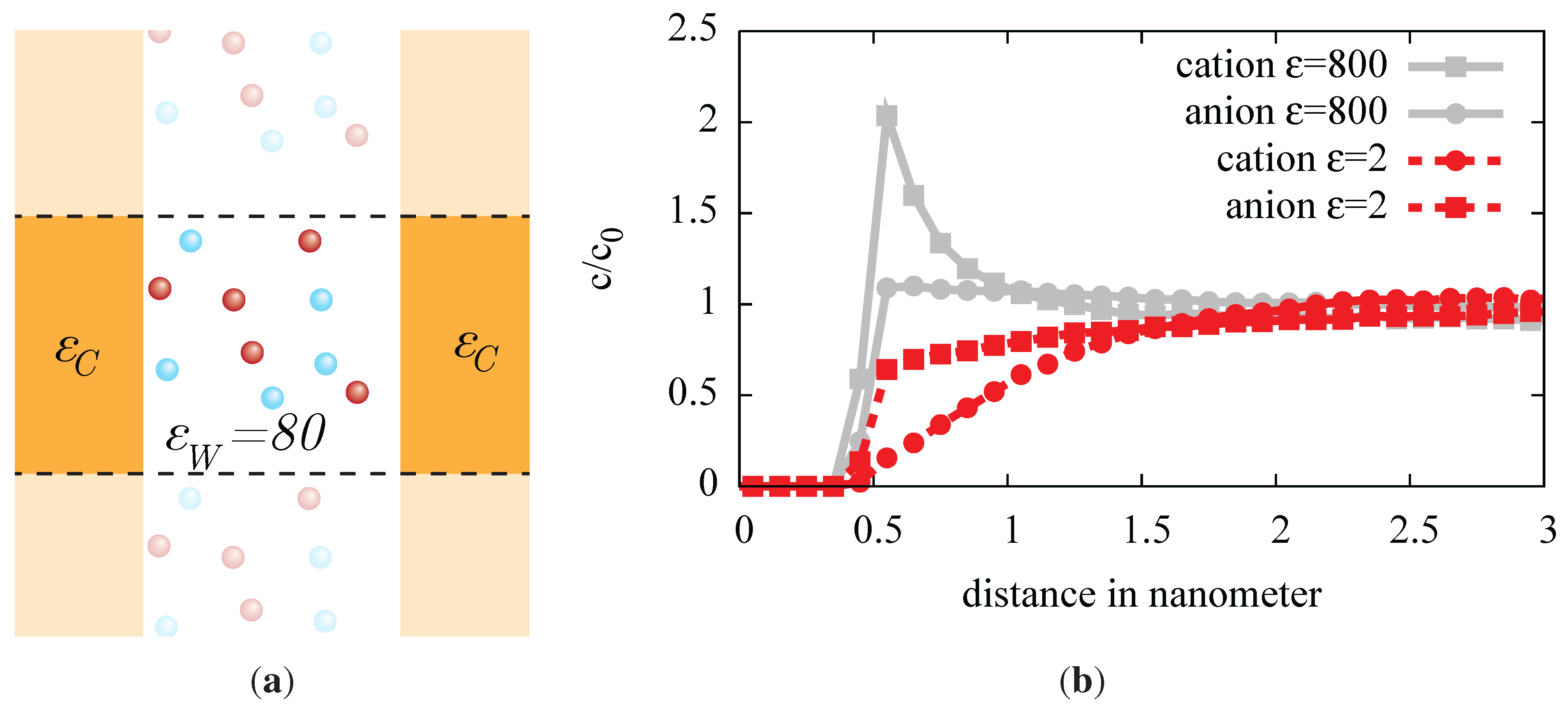
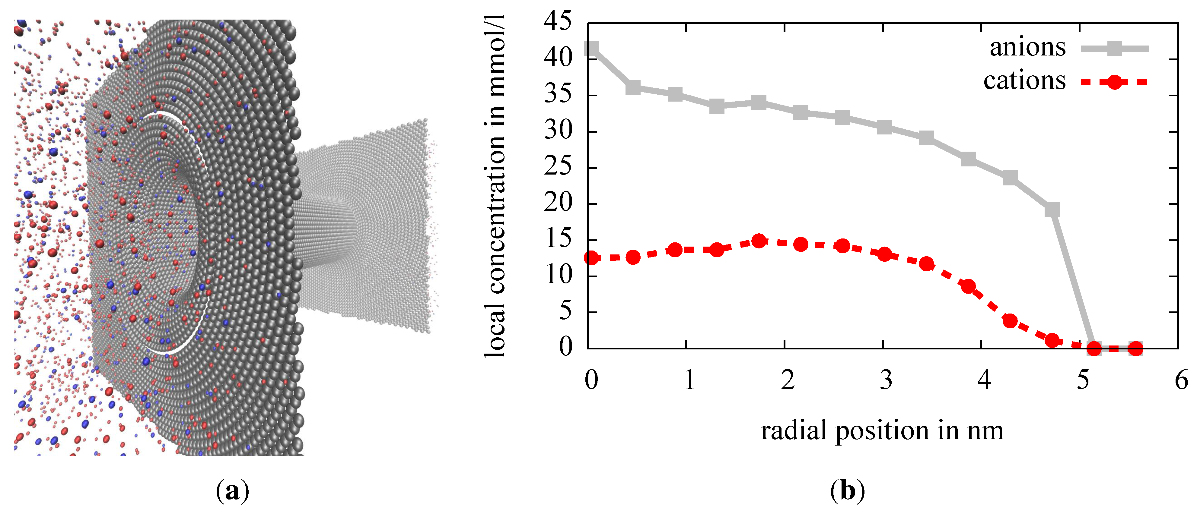
(a) Sketch of our simulation setup, a 3:1 electrolyte, e.g., AlCl, between two walls with a dielectric constant different from that of water. The size difference between the ion types is neglected in this simulation. The slab is periodically replicated parallel to the walls, vertical in the sketch. (b) Density distribution of anions and cations of the trivalent electrolyte, near the dielectric interface. The dielectric interfaces is placed at , and a repulsive potential maintains a minimum distance of 0.5 nanometers for all ions. A good dielectric , representing conducting material, strongly attracts cations, while anions are less attracted. A bad dielectric , representing a typical biological membrane, repels cations. The univalent anions are much less repelled.
Figure 2.
(a) Sketch of our simulation setup, a 3:1 electrolyte, e.g., AlCl, between two walls with a dielectric constant different from that of water. The size difference between the ion types is neglected in this simulation. The slab is periodically replicated parallel to the walls, vertical in the sketch. (b) Density distribution of anions and cations of the trivalent electrolyte, near the dielectric interface. The dielectric interfaces is placed at , and a repulsive potential maintains a minimum distance of 0.5 nanometers for all ions. A good dielectric , representing conducting material, strongly attracts cations, while anions are less attracted. A bad dielectric , representing a typical biological membrane, repels cations. The univalent anions are much less repelled.
2.1. Example: Electrolyte between Dielectric Walls
As an example application of the ICMMM2D algorithm, we simulated a 3:1 electrolyte (e.g., AlCl
) with a concentration of 0.01 mol/l confined by planar walls to a slab, as depicted in
Figure 2(a). The size difference between positive and negative ions has been neglected here. This is a good model for the narrow slit between the electrodes of a capacitor, as well as two biological membranes or glass plates. However, the dielectric properties of a metal electrode (here approximated with
) and a biological membrane (
) are very different and in both cases also differ strongly from the permittivity of the solvent; here, water (
). The resulting dielectric jumps at the surfaces have a pronounced effect on the distribution of ions near the walls.
Figure 2(b) shows this strong influence of the dielectric interfaces. Both cations and anions are attracted to the walls of high permittivity (
), but repelled by the low permittivity (
) walls. On a microscopic level, the electric field of a charge will give rise to a dielectric displacement in the wall. This displacement will weaken or pronounce the field within the dielectric medium, compared to the other side of the interface. It can be accounted for by imagining virtual mirror charges or surface charges directly on the interface. To correctly reproduce the field discontinuities at the boundary, these charges will be of an attractive nature in the region of lower permittivity and of a repulsive nature in the region of higher permittivity. Note also that the effect is more pronounced for multivalent ions. Ignoring the dielectric jumps would lead to a much more homogeneous charge distribution, so that one would strongly underestimate the effect of including multivalent ions.
3. Arbitrarily-Shaped Interfaces: Induced Charges
The concept of induced charges rather than image charges is a direct route to take into account dielectric interfaces of arbitrary shape. Conventionally, charge induction is considered to be the origin of Faraday’s cage effect: applying an electric field to a conductor will trigger the mobile charges inside to move until the electric field vanishes inside and field lines end orthogonally to the surface of induced charges. The same concept, however, can also be applied to dielectrics, hence materials with immobile charges. This can be seen from the following mathematical consideration. The Poisson equation in an inhomogeneous dielectric medium (
1) can be rewritten as:
The term,
, is identified as the
induced surface charge density,
σ. It is nonzero only on the dielectric interfaces, since
vanishes everywhere else.
Let us introduce the Green’s function,
G, for the Laplace operator. It can, e.g., be just
, but may also include the desired periodicity. Then, it is possible to eliminate the Laplace operator from the equation above and express the potential by means of two integrals:
The volume integral extends over medium 1, and the surface integral extends over all dielectric interfaces. The potential is now expressed in terms of the Green’s function of a homogeneous dielectric, yet the induced charge density,
σ, is still unknown. We now assume that the charges are embedded in a medium with permittivity,
, and for simplicity, only a second permittivity,
. By taking the gradient and inserting this expression in the definition of the induced charge density, we obtain the following integral equation:
This result is easily generalized to multiple regions with different permittivities The idea of the ICC* algorithm [
18] is to determine this charge density self-consistently, after discretizing the surface.
In principle, this approach is a boundary element method, an approach that is very widely used, e.g., for a low Reynold number flow [
29]. Different from other approaches is, however, that the efficient evaluation of the Green’s function can be borrowed from standard Coulomb solvers. This can be seen from the following: assuming a discretized surface of
m point charges on the dielectric interface, the equation above for discretization point
k can be written as:
where
is the surface area of the surface element,
k. The term in square brackets is just the electric field acting at the position of point
k, assuming a homogeneous dielectric constant,
, in the system, created by conventional (not induced) charges. Any standard Coulomb solver can thus be used to perform the calculation. The desired solution of all
is the fix point of the following iteration:
It turned out that this iteration is very stable and with a choice of , no stability issues occur. In every MD step, only 1–3 iterations are necessary, as the particle positions change only slightly.
An important advantage of this algorithm is that the computationally most costly part, the evaluation of the electric field, can be done with
any usual electrostatics solver without modifications. Thus, not only the computational efficiency, but also the periodicity is inherited from the Coulomb solver. The complexity of the algorithm remains unchanged by the presence of induced surface charges. However, the number of particles can increase considerably. We found it sufficient to discretize the surface with mutual particle distances equal to the distance of closest approach. For the system shown in
Section 2, this would mean, in total, 1,600 surface charges per wall, compared to less than 100 ions in the system.
In our research, this algorithm was applied to investigate if dielectric effects can change the electrolytic conductance of very narrow pores, nanopores, through membranes or have an influence on the translocation of charged macromolecules through nanopores [
19,
30]. Here, dielectric boundary forces lead to a repulsion of (unpaired) ions. Taking into account dielectric effects in small pores will decrease the number of available ions and, thus, decrease the conductance.
The error in the obtained electric field depends on the applied resolution with which the surface is resolved. The method has been tested for planar and curved surfaces [
18], and it was found that from a distance larger than one lattice spacing, the relative error remains smaller than 1%. Since the permissible error depends often on the desired application, we advise to determine the necessary accuracy specifically for each case. If interfaces with media with a high dielectric constant or even metallic boundaries are considered, charges are attracted to the surface and can come quite close to the interface, depending on the ion size. In this case, the necessary accuracy is clearly higher than for interfaces with lower dielectric media, from which particles are repelled.
3.1. Example: Ion Distribution in a Pore
As an example, we investigate the ion distribution in a cylindrical pore of radius 5
in a 40
-thick membrane in an aqueous electrolyte. This geometry resembles the so-called solid state nanopores [
31,
32,
33] in silicon wafers. In several experiments (e.g., [
34,
35]), it was shown that single DNA molecules present in such a pore can be detected by the change of the electric conductance of such a system. To make the dielectric effect more pronounced, we again used a 3:1 electrolyte with a concentration of 10
. Our setup is sketched in
Figure 3(a): the surface charges of the ICC* algorithm are displayed along with the ions, each as spheres. We assume the dielectric constant of the membrane to be
. In
Figure 3(b), the equilibrium distribution of ions near the center of the pore is shown. Ions, especially the trivalent ones, are repelled from the dielectric interface. This leads to an overall decrease of ions in the pore by around 20%. Thus, the conductance of the system can be expected to be reduced similarly, compared to a model that does not consider the dielectric contrast.
Figure 3.
(a) The induced charge calculation (ICC*) example system: positive and negative ions are displayed as red and blue spheres, the ICC* discretization points by grey spheres; (b) ion density of both species in the pore measured close to the center of the pore.
Figure 3.
(a) The induced charge calculation (ICC*) example system: positive and negative ions are displayed as red and blue spheres, the ICC* discretization points by grey spheres; (b) ion density of both species in the pore measured close to the center of the pore.
4. Metallic Interfaces: Corrections
Metallic boundary conditions are the
limit of Equations (
2) or (
11), where
ε denotes the dielectric constant of the surrounding medium. The corresponding dielectric contrasts become
, so that the field automatically vanishes in the conductor. In the case of two dielectric interfaces, this simply leads to constant potentials on each of the two interfaces, but the potentials are not necessarily the same. It is, however, also possible to fix the electrostatic potential on surfaces in periodic systems. This has been done, for example, for the Monte Carlo implementation of the local algorithm presented in
Section 5 [
13,
14]. The fixing of the surface potential in periodic systems can be achieved also for other algorithms, but the details are different, and we therefore briefly describe the necessary ingredients for the algorithms previously described.
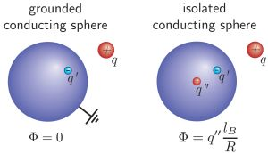
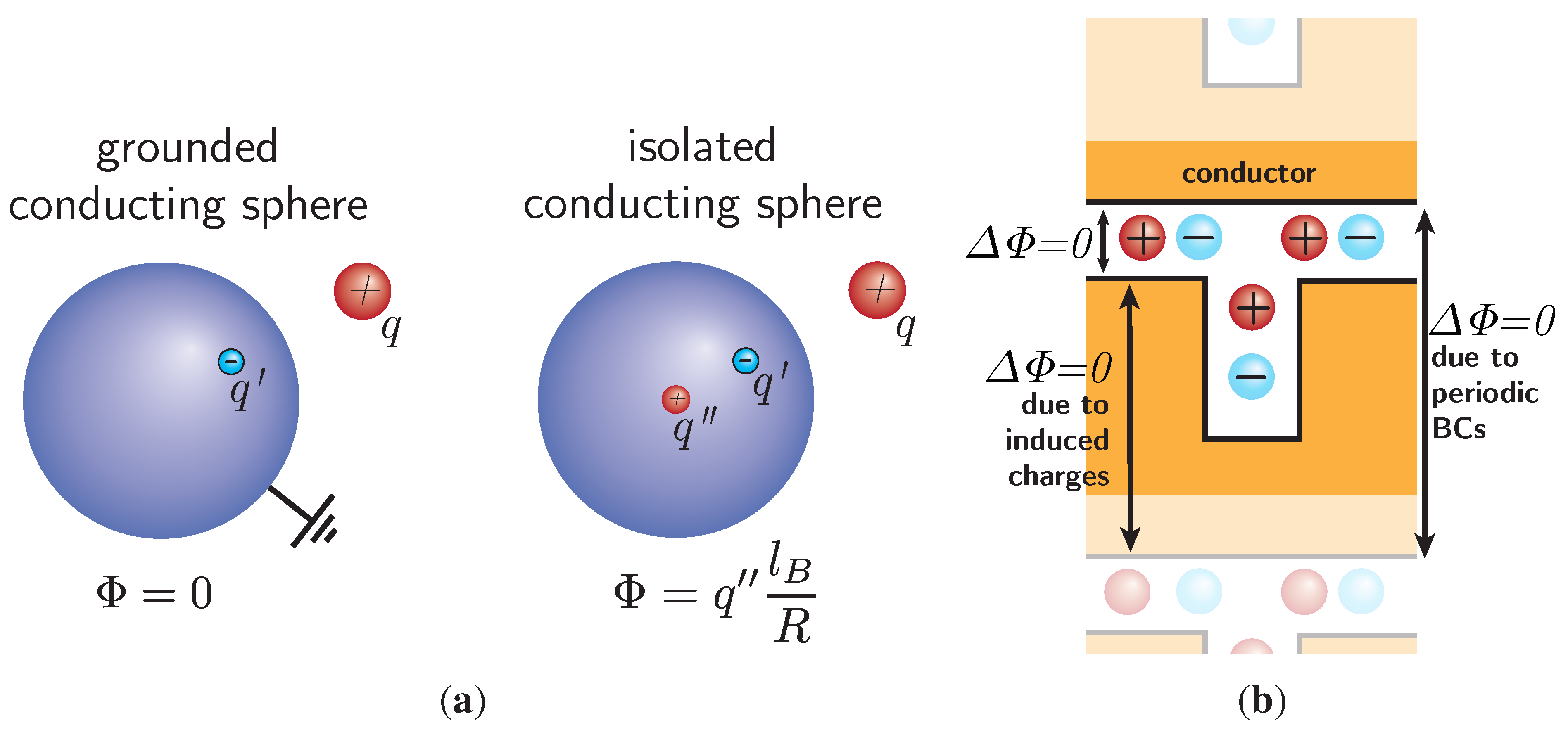
The starting point is the textbook example of a single point charge outside of a conducting sphere, as depicted in
Figure 4(a). A metallic sphere brought into an electric field can either be isolated, i.e., the charge on the sphere is constant, or on a constant electrostatic potential, typically grounded. Again, the boundary problem can be solved by adding an image charge opposite to the source charge in the sphere. This ensures that the surface potential of the sphere does not vary. A second image charge can be placed at the center, which dictates the electrostatic potential at the surface of the sphere: for an isolated sphere with zero net charge, the image charge at the center must be of the same magnitude as the other image charge, but with the opposite sign. For a grounded sphere, it is simply zero. In the following, we will show how conducting or grounded boundary conditions can be added to both the image charge and induced charge methods, in order to perform computer simulations with constant electrostatic metallic surface potentials.
Figure 4.
(
a) Illustration of the dielectric boundary problem of single charge
q outside of a grounded conducting sphere. The problem can be solved by assuming an image charge,
, inside the sphere, leading to zero potential Φ on its surface. If the sphere is assumed to be conducting, but isolated, the excess charge,
, has to be canceled by adding a second charge,
, in the center of the sphere, which leads to a constant surface potential, Φ. (adapted from [
25]). (
b) A more complex geometry with an upper and lower electrode (yellow). The electrodes are treated with the ICC* algorithm. If a Coulomb solver with periodic boundary conditions (BCs) in the vertical direction is applied, the potential difference between both electrodes is automatically zero. This is because the periodicity yields zero potential difference between an electrode and its periodic image, and the ICC* algorithm ensures that the two electrodes connected over periodic BCs are on equal potential.
Using the MMM2D far formula, the potential difference between the two plates appears as the
mode of the electrostatic potential, i.e., the
term in Equation (
5). The higher modes, in the limit of
, serve to hold the potential constant on each conducting plate individually. Due to the absolute value, this term does not cancel when considering the interactions in the primary box. The potential difference,
V, of the two plates is:
where
ρ denotes the charge density. In terms of the
z-component of the dipole moment of the system,
, this equals:
since the
contribution vanishes once more due to charge neutrality. In order to cancel this potential difference, one has to apply a constant external field
=
in every MD step. This additional field corresponds to that created by the central charge in the spherical image charge picture, which puts the surfaces to equal potential. To obtain a different fixed potential
, an additional field,
, needs to be applied in the
z direction.
Systems treated with ICC* require no special measures if the surface on the constant potential is connected within the simulation box. However, some attention is required when considering electrodes at the boundary of the simulation box, as depicted in
Figure 4(b). If an electrostatics method is applied that is not periodic in the respective direction, this will result in two electrically unconnected surfaces. To obtain electrically connected surfaces, such as two grounded plates, it is sufficient to use a solver periodic in the required direction and to leave a gap in the periodic images. This can be seen from the simple case depicted in
Figure 4(b). If a periodic solver with metallic boundary conditions is used, for example, the Ewald summation, the difference between the electrostatic potential at a given position and its nearest periodic image is necessarily zero, due to periodicity. However, since the induced charges create a constant potential in both sections of the conductor, these must be the same throughout the whole, periodically connected conductor.
To obtain a non-zero electrostatic surface potential, the solution of the Poisson equation with zero potential can be superimposed with a solution of the empty simulation box with nonzero potential on the surfaces. This requires a solution of the Laplace equation that is then applied as an external field, just as in the simple case of parallel plates. To do that, our simulation package, ESPResSo, supports reading in tabulated external potentials, which are applied to charged particles weighted with the according charge. It also takes care that the external potential is not applied to image charges. The solution of the Laplace equation has to be obtained externally. We use a finite element solution based on the DUNE framework [
36,
37]. Packages, like Matlab or Comsol, can, of course, also be applied.
4.1. Verification: Field and Potential in Metallic BCs
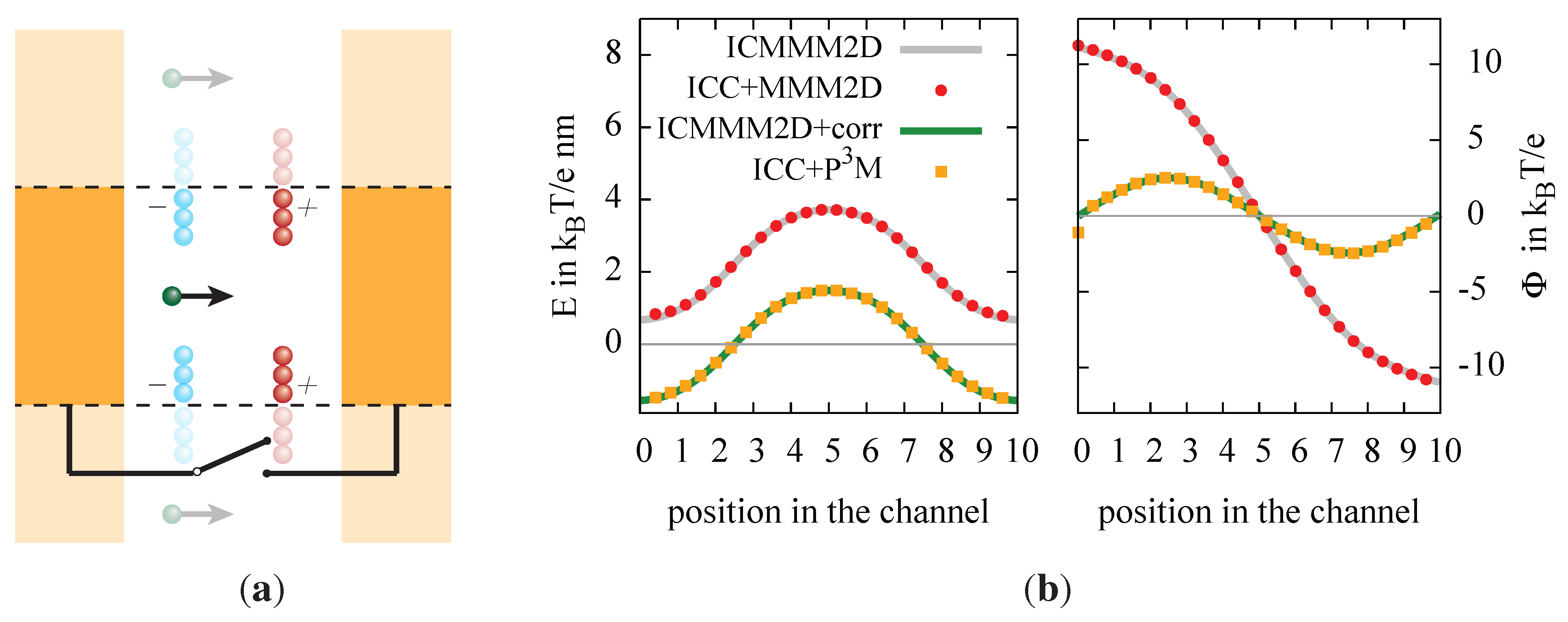
In order to illustrate the methods described above, we show its importance on a simple model system. We chose a planar geometry, because in this geometry, it is possible to use both the image charge method, as well as the induced charge method. Thus, our system consists of a set of charges confined by two parallel conducting planes. In the following, we will show that isolated plates can be simulated either by using the ICMMM2D algorithm without correction or by using the ICC* method with a Coulomb solver, which is not periodic in the direction of the planes’ normal vectors. Connected plates at zero potential difference can either be simulated using the ICMMM2D method with the correction derived above or using the ICC* method with a Coulomb solver, which is periodic in the normal direction. As a solver for the fully periodic case, we use the P
M algorithm [
8,
38]; as a solver for the partially periodic case, MMM2D [
26,
27].
For simplicity, we construct a constant charge distribution with a net dipole moment and probe the electrostatic field with a small test charge
that is moved through the system. Metallic boundary conditions are created at
and
by using the four algorithms described above. The dielectric permittivity between the surrounding metal plates is assumed to be
for bulk water. The charge distribution we chose is depicted in
figure 5(a): fixed, charged particles form two oppositely charged plates at
and
. In one of the two directions parallel to the surrounding metal plates, a void of a length of 0.5
is left, so that the test charge can be moved through the gaps without getting close to the charged plates. We measure the electric field by performing a force calculation with the respective algorithm and dividing the obtained force by the small value of the test charge. In
Figure 5(b), we report the measured electric field and the potential obtained from the integration of the electric field. We observe the expected behavior: the shape of the electric field is identical in all cases up to a constant. In the cases where the the algorithms are supposed to simulate two connected metal electrodes, the electric field is shifted downwards, so that the integral is zero, and both electrodes have the same potential.
Figure 5.
(a) Sketch of the model system that was used to probe the influence of grounded and isolated metallic boundary conditions. The two possible setups are depicted by adding a switch to electrically connect the two plates. (b) The resulting electrostatic field, E, perpendicular to the plates and the electrostatic potential in the slab.
These two methods are, in our opinion, very interesting for investigating supercapacitors based on electrolytes or ionic liquids, (e.g., [
39,
40,
41]). They are complimentary in the sense that the image charge method is computationally very cheap: the extra cost of image charges is typically negligible, and the only model parameter is the distance of closest approach between ions and the metallic interface. The induced charge methods, however, allow for arbitrarily-shaped surfaces, and one can investigate very complex geometries. The extra computational cost is feasible if the resolution of the surface can be relatively coarse or, in other words, a certain electrostatic “roughness” or inaccuracy is acceptable and can be considered as an adjustable model parameter.
5. Smooth Variations: Local Method
We have presented methods to deal with sharp dielectric interfaces of several types and shapes. Yet, none of these methods offer the possibility of a spatially smooth varying permittivity. More precisely, they are all restricted to single step-like changes and do not allow charges to pass through those regions of variation.
In the following, we sketch an algorithm that allows for an arbitrary distribution,
, of the permittivity that we call Maxwell Equations Molecular Dynamics (MEMD). The concept of diffusive field propagation was first presented by Maggs in 2002 [
20,
42] and adapted for molecular dynamics simulations simultaneously by Rottler and Maggs [
43] and Dünweg and Pasichnyk [
21]. The algorithm is not based on the static Poisson Equation (
1), which is of a global nature. Instead, the time derivative of Gauss’ law
of electrodynamics, with
, is extended to the following constraint of the most general form.
where
denotes the local electric current and Θ is an arbitrary vector field representing an additional degree of freedom. If we apply this constraint to the system propagation via a Lagrange multiplier,
, fix the gauge degree of freedom from Equation (
13) to:
and introduce the magnetic field,
, then this so-called temporal (or Weyl) gauge will, via variational calculus, lead to the equations of motion for the charges and fields that are known as the Maxwell equations. The actual electrostatic potential, Φ, is never calculated in this algorithm, only the electric field,
, for Lorentz force calculation:
It is remarkable that simply by applying constraint (
13) and the Weyl gauge, (
14), the complete equations of the electromagnetic formalism can be reproduced. It can even be shown [
20] that the propagation speed of the magnetic field, an equivalent of the speed of light,
c, can be reduced in a Car-Parrinello manner, and correct retarded solutions for statistic observables can still be maintained.
This reduces the elliptic partial differential Equation (
1) to a set of hyperbolic differential equations for the propagation of magnetic fields and charges, requiring only local operations for the solution. It therefore opens up the possibility of arbitrary local dielectric permittivities within the system. If discretized on a lattice and coupled with a linear next neighbor interpolation scheme for the charges and electric currents, the permittivity can be set individually on every lattice link [
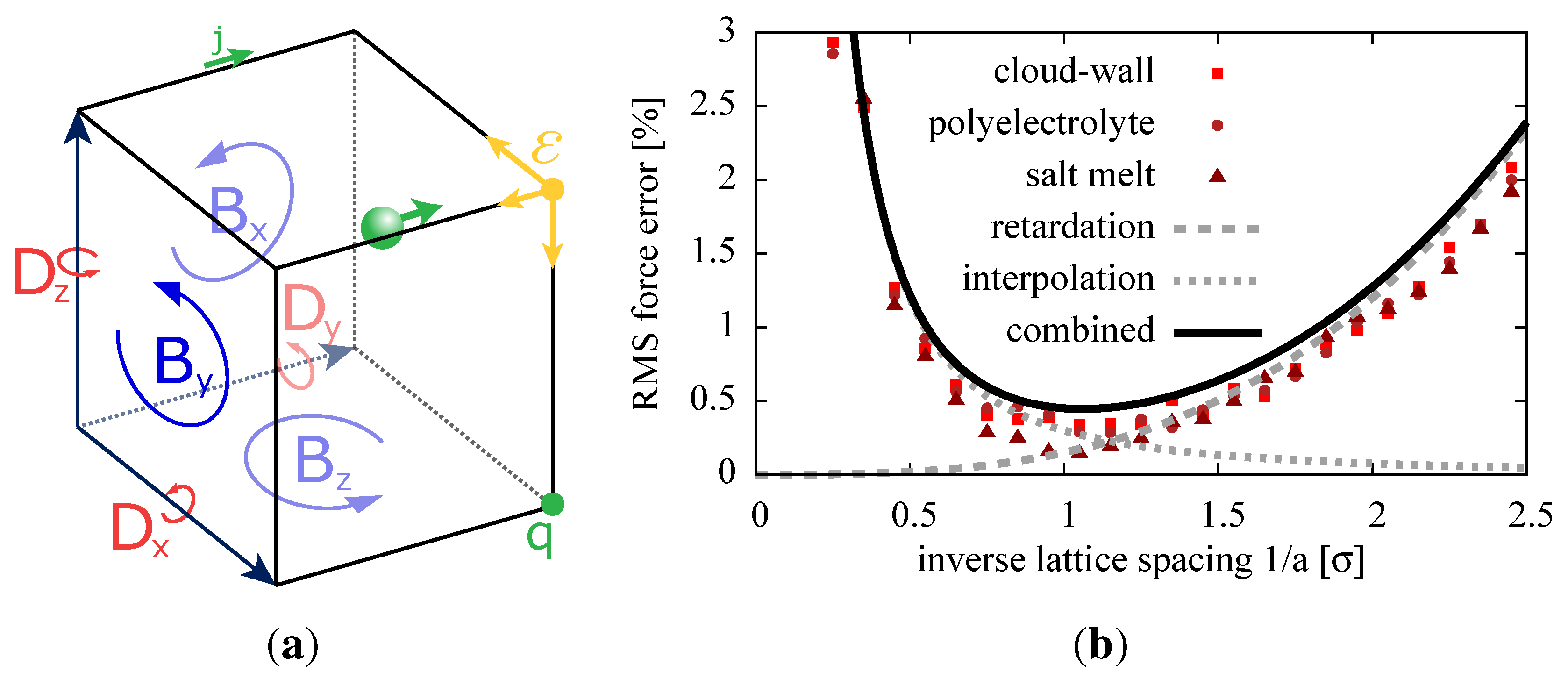
44]. The discretization is carried out as seen in
Figure 6(a). This is in agreement with
being a differential one-form, if we assume the tensor to only have identical diagonal entries (optically isotropic dielectric medium).
In this algorithm, the charges can move freely through a smoothly varying dielectric medium. At the current implementation state, the variations are only spatial, but temporal changes of the dielectric during the simulation are theoretically possible. It has also been shown that the field propagation within the system reproduces the classical Keesom potential interactions between two dielectric interfaces [
45].
Figure 6.
Maxwell Equations Molecular Dynamics (MEMD) interpolation of the charges onto the lattice. (a) The electric current, , permittivity ε and electric field are interpolated to the adjacent lattice links. The magnetic field component, , is placed on the lattice plaquettes via a finite-differences curl operator. (b) The numerical error of the algorithm is dependent on the lattice spacing. The error can be reduced by applying a coarser mesh, coming from the right in this graph, and, thereby, increasing the field propagation speed in the system. However, at large lattice spacings a, the interpolation error at small distances dominates and diverges. In a densely-populated system, like the examples seen here, a minimal relative error of is achieved at mesh sizes comparable to the minimum distance of two charges, denoted here by σ. For reference, the errors compared to a high precision P3M force calculation are included for three example systems.
One source of numerical errors in this algorithm stems from the retarded solution of the Maxwell equations with the Lorentz force calculation (
16) at the finite speed of light
. The second error is introduced via the linear lattice interpolation of the charges. The self-interaction of a charge with the lattice can be corrected, for example, using a lattice Greens function for constant dielectric backgrounds, but for locally varying dielectric properties, the implementation relies on a straight-forward direct subtraction scheme. Here, the local electric field created by the interpolated charges of one particle is calculated and subtracted from the resulting force. Still, an interpolation error remains for the coupling between two particles at close distances, since the charge is spread out on the lattice.
Since the field propagation speed within the system is proportional to the lattice spacing,
a, the first of these errors depends on
(see Equation (
16)), whereas the second error for geometrical reasons scales like
. It can be seen in
Figure 6(b) that the error can be reduced by making the mesh coarser, until the interpolation error at close distances dominates for a very coarse mesh. The plot shows a theoretical estimate of the error and simulation data for three example systems: an artificial system with a charged infinite plate (cloud-wall), a polyelectrolyte in aqueous solution and a silica salt melt. The second parameter, besides the lattice spacing, the artificial speed of light,
c, was chosen to obey the Courant-Friedrichs-Lewy stability condition,
, where
is the time step of the MD simulation. For every lattice spacing, there exists a maximum speed of light parameter that keeps the algorithm stable. Here, we picked the speed of light
as the parameter for all three setups. It turns out that a relative force error of
is achievable in sufficiently homogeneous systems, and the optimal lattice spacing is comparable to the minimal distance between charges. The interpolation error, and, therefore, the total error, can be reduced by splitting off a near field that spans across multiple mesh cells and applying a short-range calculation in this region. However, this is not possible for spatially varying permittivity and will not be discussed here.
5.1. Example: Colloid with Dielectric Jump and Continuous Dielectric Constant
An example where such smoothly varying changes in
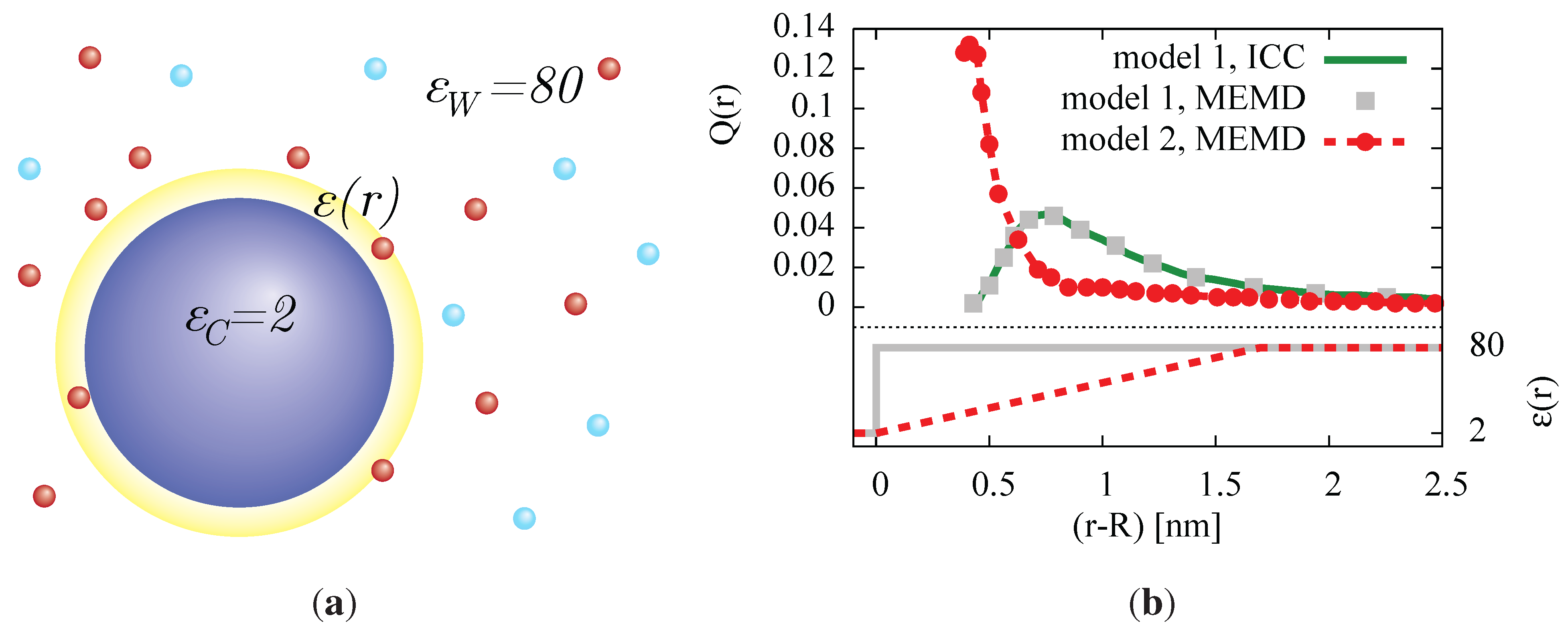
ε can play a substantial role is the simulation of a charged colloid in a salt solution (
Figure 7(a)). The first approach at dielectric coarse graining is a sharp dielectric contrast between the colloid and the solvent. Such a system can be simulated by the ICC* method presented in
Section 3 with a dielectric permittivity
within the colloid and
for the surrounding bulk water. However, in practice, the polarizability, and, therefore, bulk permittivity, of water close to charged surfaces and in regions of high ion concentrations is significantly reduced [
46]. Many workarounds were proposed to address this behavior, including the introduction of an artificial Stern layer [
47] to reproduce the desired Gouy-Chapman predictions. A more direct and more physical approach is to interpolate the bulk permittivity from the colloid to free water between the colloid surface and the solution (see the bottom of
Figure 7(b)). A linear interpolation is sufficient to describe the local permittivity obtained from atomistic simulations [
48].
Figure 7.
(a) A charged colloid (charge , radius ) is suspended in a salt solution (concentration ). The dielectric constant is modeled as an abrupt jump to the bulk water permittivity with the MEMD and ICCPM algorithms (gray points, green curve) or a linear radial increase within two ion diameters from the colloid surface between the two regimes (red). (b) The resulting radial charge density profiles, which exhibit a drastic difference between the dielectric jump in model 1 and a smooth interpolation in model 2.
In order to illustrate the difference between dielectric jump and continuous dielectric constant, we simulated a spherical setup with two different models of radial permittivity dependence
. Model 1 includes a discontinuity of
ε at the colloid surface, whereas model 2 uses a linear interpolation
over four ion radii
. Model 1 additionally has been simulated using the ICC* algorithm combined with the P
M Coulomb solver, for comparison.
Figure 7(b) shows the radial charge density of the counterions around a colloid of charge
with radius
in a monovalent electrolyte solvent of
concentration. The difference between the two models is drastic and can be explained by the stronger Coulomb attraction of counterions towards the colloid, due to the smaller dielectric permittivity close to the colloid surface. Another effect is the earlier occurrence of overcharging effects, because of increased ion correlations, due to their entering the region of lower permittivity. The comparison with the ICC* algorithm, on the other hand, shows that MEMD is also very well capable of simulating dielectric jumps, provided a sufficiently small mesh, comparable to the particle size, for the discretization of the electrodynamic equations can be realized. The computational overhead, compared to a simulation with MEMD at constant background permittivity, is negligible at less than
in this setup. MEMD ran
longer than the identical setup for the ICC* algorithm. This overhead could be reduced by further optimizing the mesh size, which was chosen to be well resolved here at a colloid diameter of 16 mesh spacings.
6. Conclusion
In this review, we have presented several methods to compute electrostatic interactions in the presence of dielectric interfaces in computer simulations and give examples that demonstrate the importance of taking the dielectric contrasts into account, like they appear in implicit solvent models.
In a planar slit pore, such as a plate capacitor, ions are attracted to the walls or are repelled by them, depending on whether the walls consist of an dielectric medium with high or low polarizability. The presented ICMMM2D [
16] or the ELCIC [
17] algorithms allow one to treat a slit pore with dielectric jumps at both confining interfaces, like capacitors or thin films.
In curved or more complex geometries, such as a nanopore, dielectric properties can also drastically alter the ion distribution or the translocation properties of charged macromolecules. The presented ICC* algorithm allows one to include arbitrarily-shaped dielectric interfaces in computer simulations, by computing the induced surface charges necessary to fulfill the dielectric boundary conditions on the fly.
As another interesting application, we presented the example of plates that are held electrically at a constant potential, such as one would use to study capacitors. This will lead to a different polarization than isolated grounded plates, and this effect has to be taken into account in simulations, with algorithms that are adjusted accordingly. Both the ICMMM2D and the ICC* algorithm can handle this special case, as we have demonstrated.
Finally, we have shown that smoothly varying dielectric properties again are very different from dielectric jumps as treated by ICMMM2D or ICC*. At present, only the sketched MEMD electrostatics algorithm [
20,
21,
44] is able to treat such systems.
All algorithms presented here, including the extensions for varying dielectric constants, are implemented in the open source simulation package, ESPResSo [
22,
23]. MEMD is also part of the open source ScaFaCoS (Scalable Fast Coulomb Solvers) library for fast Coulomb solvers [
49]. In conclusion, computational tools for the most common cases of varying dielectric properties are readily available for computer simulations. This will become more and more important with the increased interest of applying coarse-grained or implicit solvent models in nanopores, biological membranes, thin films and supercapacitors.


